Latent Space Perspicacity and Interpretation Enhancement (LS-PIE) Framework

Abstract

Linear latent variable models such as principal component analysis (PCA), independent component analysis (ICA), canonical correlation analysis (CCA), and factor analysis (FA) identify latent directions (or loadings) either ordered or unordered. These data are then projected onto the latent directions to obtain their projected representations (or scores). For example, PCA solvers usually rank principal directions by explaining the most variance to the least variance. In contrast, ICA solvers usually return independent directions unordered and often with single sources spread across multiple directions as multiple sub-sources, severely diminishing their usability and interpretability. This paper proposes a general framework to enhance latent space representations to improve the interpretability of linear latent spaces. Although the concepts in this paper are programming language agnostic, the framework is written in Python. This framework simplifies the process of clustering and ranking of latent vectors to enhance latent information per latent vector and the interpretation of latent vectors. Several innovative enhancements are incorporated, including latent ranking (LR), latent scaling (LS), latent clustering (LC), and latent condensing (LCON). LR ranks latent directions according to a specified scalar metric. LS scales latent directions according to a specified metric. LC automatically clusters latent directions into a specified number of clusters. Lastly, LCON automatically determines the appropriate number of clusters to condense the latent directions for a given metric to enable optimal latent discovery. Additional functionality of the framework includes single-channel and multi-channel data sources and data pre-processing strategies such as Hankelisation to seamlessly expand the applicability of linear latent variable models (LLVMs) to a wider variety of data. The effectiveness of LR, LS, LC, and LCON is shown in two foundational problems crafted with two applied latent variable models, namely, PCA and ICA.

1. Introduction

Latent variable models are statistical models that describe the relationships between observed and unobserved, or latent, variables. These models assume that the observed variables are generated by underlying latent variables, which are not directly measured or observed but are inferred from available data [1,2]. Figure 1 (adapted from [3,4]) depicts the encoding process of linear latent variable modelling by taking a high-dimensional input signal and transforming it into a lower-dimensional latent space, shown here as a three-dimensional latent representation. Consider Figure 1a, the three-dimensional latent representation indicated by the axes $X-Y-Z$ that is projected onto Figure 1b: the $X-Y$ plane, Figure 1c: the $Z-X$ plane, and Figure 1d: the $Z-Y$ plane. The variation in projected latent structure for the same data is evident. This warrants whether grouping, scaling, and projecting various latent dimensions can enhance the informativeness of the latent space. Practically, latent variable models (LVMs) can be classified into reconstruction- and interpretation-centred models [4].

Reconstruction-centred LVMs identify compressed latent representations that efficiently reconstruct variance in the data, often optimal for the given model’s flexibility. In turn, interpretation-centred LVMs attempt to identify interpretable latent presentations, e.g., independent variance contributing sources, when explaining the variance in data. The latter often results in less compressed latent representations. The importance of organising latent spaces can be seen in Figure 1. This figure shows that certain structures are lost when data are projected on different planes. However, certain latent representations still contain more structure than others.

The tasks of these two approaches are distinct: reconstruction-centred models are efficient at compressing data into lower dimensional latent spaces for efficient reconstruction, while interpretation-centred approaches aim to identify lower-dimensional latent spaces that are interpretable, where contributing factors or sources of variance in the data are independent and untangled [4].

Reconstruction-centred LVMs usually present their latent directions, which are ordered from explaining the most to least variance or vice versa. These include singular value decomposition (SVD) [5,6], principal component analysis (PCA), and conventional singular spectrum analysis (SSA) [7,8], giving clear discernibility to reconstruction-focused latent representations. Ironically, interpretation-centred LVMs usually return unordered latent directions, with  single sources spread across multiple directions, making these latent representations less informative and more difficult to discern, interpret, and manage. These include independent component analysis (ICA) [9,10,11], with a variety of underlying objective functions to be maximised such as non-Guassianity measures or proxies such as negentropy, skewness, kurtosis, or minimisation of mutual information between latent variables.

This paper examines the impact of applying techniques such as latent scaling (LS), latent ranking (LR), latent clustering (LC), and latent condensing (LCON) to the latent spaces generated by linear LVMs that traditionally do not incorporate them. Applying these methods improves the interpretability of the generated latent representations. It allows for greater flexibility in analysing various datasets and generating richer and more informative latent representations. As shown in Figure 2 these four algorithmic approaches are combined into the LS-PIE module.

Four transformations are proposed to improve the post-processing and identification of latent representation. Latent ranking (LR) and scaling (LS) rank and scale latent directions based on specified metrics, while latent clustering (LC) compresses the latent space using clustering for a user-specified number of clusters. In contrast, latent condensing (LCON) enables optimal latent discovery by estimating the optimal number of clusters to enhance the interpretability and usability of latent space representations.

In this case, the ranking and scaling methods (LR, LS), as seen in several methods such as PCA, are more widely applied, and clustering methods are explored to examine the underlying latent structure. This has been further expanded on using the underlying structures to perform follow-up analysis to minimise the discovered latent spaces (LC, LCON). These enhancements can be applied to latent spaces resulting from reconstruction-centred and interpretation-centred LVMs to re-rank already ordered latent variables according to an alternative metric, to order unordered latent variables, or to interrogate the influence of pre-processing or filtering of data on latent interpretability [12], just to mention a few use cases. These cases have significant practical and research implications and have yet to be explored in depth.

The effectiveness of these analysis methods is showcased in two crafted foundational problems for two applied latent variable models: PCA and ICA. These two methods have been chosen because they represent reconstruction-centred and interpretation-centred LVMs.

2. Required Background

2.1. Latent Variable Models

Auto-association [13] or auto-encoding [14] is a fundamental concept in LVMs to make the unsupervised learning problem of finding an appropriate latent representation tractable. A conceptual outline of auto-encoding is shown in Figure 3, which depicts encoding and decoding. Encoding transforms higher-dimensional input data into a lower-dimensional latent representation, while decoding transforms the latent representations of higher-dimensional data back to their higher-dimensional representations. Variance-driven LVMs compress input data into compact latent representations. In contrast, source-driven latent representations aim to identify informative latent representations that indicate sources contributing to the variance in data.

Inferencing on latent or reconstructed representations enables latent and reconstruction inferencing, respectively. This framework aims to enhance the latent representations of LVMs for improved and enhanced latent inferencing.

We use a set of time-series data represented by an $m\times n$ matrix $\overline{\mathit{X}}$, where m is the number of observations and n is the number of variables or the discrete times at which data are recorded. For time-series data, the former relates to the number of samples, while the latter relates to the time length of each sample. Latent variable models typically proceed as follows

• Data standardisation through mean centring or whitening of the data, $\mathit{X}$.
• Compute the $n\times n$ covariance matrix $\mathit{S}$ of the standardised time-series data $\mathit{X}$.
• Find latent directions for the data $\mathit{S}$ by maximising or minimising an objective function plus regularisation terms subject to equality (equality constraints between latent directions are often enforced, e.g., orthogonality of the latent directions or some transformed representation of the latent directions. This can always be solved by direct optimisation, but solving the first-order necessary optimality condition, or a matrix decomposition may in some cases be computationally more efficient [15]) and inequality constraints [15]. PCA diagonalises the covariance matrix by finding its eigenvectors and eigenvalues, where eigenvectors represent the principal components and eigenvalues represent the variance each principal component explains.
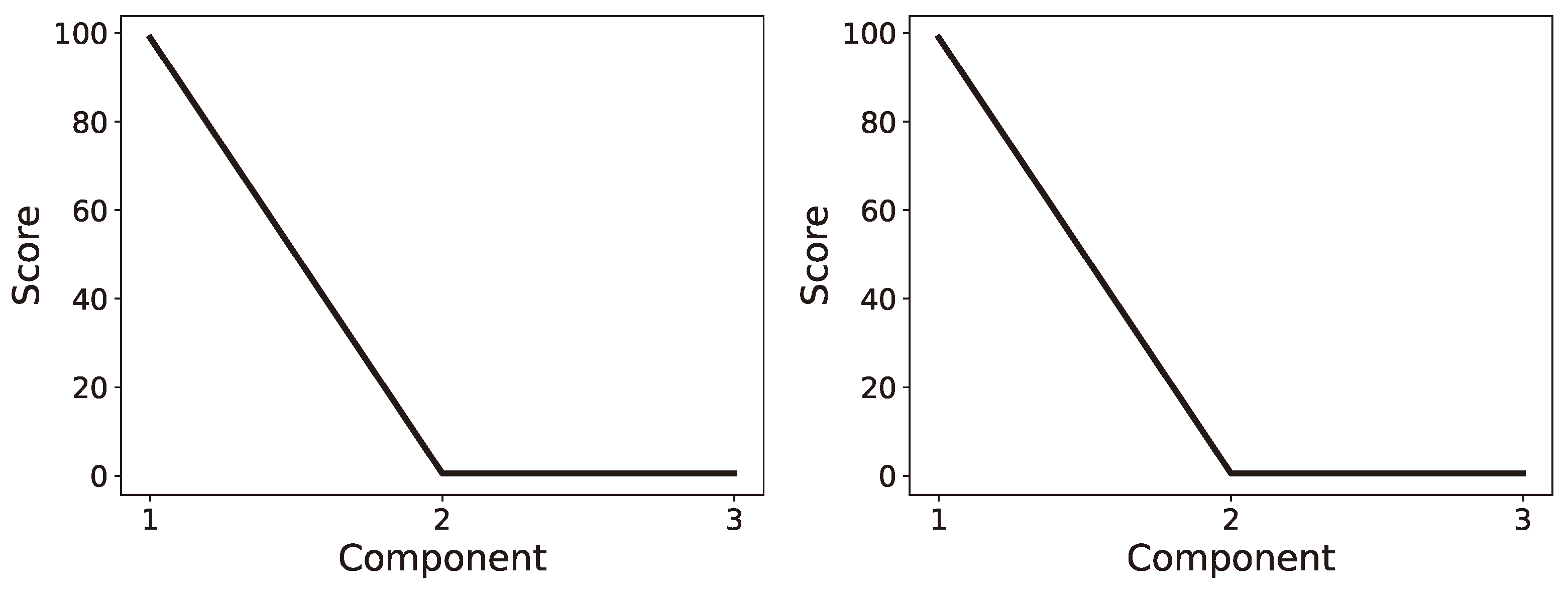
• Select k latent directions from a maximum of $rank\left(\mathit{S}\right)$. Eigenvalues and their associated eigenvectors are automatically sorted in descending order, from which k eigenvectors associated with the largest eigenvalues are usually selected. By choosing eigenvectors corresponding to the largest eigenvalues, the LVM prioritises reconstruction as they capture the most significant variation in the time-series data.
• The latent representation for a sample is obtained by projecting standardised time-series data $\mathit{X}$ onto k selected latent directions (a.k.a. loadings) to obtain a k-dimensional latent representation of the sample often referred to as a k-dimensional score.
• Reconstructing the sample from the latent representation merely requires the summation of each component of the k-dimensional score multiplied by their respective latent direction.

LVMs have seen increasing use in various fields with the advent of deep learning. These faster, larger models have allowed for research into learning sequential probabilistic models from high-dimensional data, such as audio and video [16]. The rise of new models has allowed for advancements across personalised medicine, electronic health record analysis, and epidemiology in a wide range of scientific fields wherein the recovery of latent generative causes for observed phenomena [17]. These models are especially effective in fields wherein large datasets must be analysed, e.g., medical research [18]. Of these approaches, few have seen as much success as autoencoders, a family of unsupervised learning methods that use neural network architectures to learn lower-dimensional, latent representations of input data. These models have found widespread use in prediction and classification across a wide range of fields [19,20]. These models traditionally require large networks to function accurately.

Recent innovations in LVMS include lightweight deep LVMs (LDLVMs). These aim to combine the robustness of deep LVMs while mitigating drawbacks. Deep LVMs such as autoencoders (AEs), variational autoencoders (VAEs), and deep belief networks (DBNs) apply industrial modelling tasks, including fault diagnosis, prognostics health management, and soft sensor development. LDLVMs aim to perform these tasks with significantly smaller network sizes, which require less intensive training [21]. Other LVMs investigated are singular spectrum analysis (SSA), a model analogous to PCA but designed to be applied to time-series data. The primary aim of SSA is to decompose a given time series into a small number of easily understandable components, such as slowly changing trends, oscillatory components, and noise. These models are increasingly used across various fields, including financial time-series analysis. Methods like filter-adjusted oblique SSA (FOSSA) and iterative oblique SSA (IOSSA) have been introduced to aid automatic trend identification [22,23].

Unsupervised LVM methods such as ICA have been extended to non-linear data to perform non-linear blind source separation (BSS). These problems are particularly challenging due to their non-unique solutions without additional constraints or regularisation, often addressed through Bayesian inference methods. Extensions to FastICA allow for better modelling of higher dimensional latent systems, including independent subspaces with decoupled dynamics, canonical correlation analysis, and projective non-negative matrix factorisation (P-NMF). These approaches have been applied in telecommunications and climate data analysis, illustrating their practical utility [24].

Other approaches have been explored to extend latent models to higher dimensional, multi-variable arrays. This includes Tucker3 or N-Way PCA and PARAFAC (parallel factor analysis). Tucker3 is a basic multi-way model originating from psychometrics and commonly used in chemometric analysis. Proposed as a model for three-mode factor analysis it acts as extension of PCA [25], it has since found application in the fields of chromatography, environmental analysis, and perception analysis. This widespread use has meant that the need for efficient algorithms for large data sets is of the utmost importance and several algorithms have been described based on least squares regression, singular value decomposition, Gram–Schmidt orthogonalization, or a modified Bauer–Rutishauer BR estimation [26]. It has also been applied to compositional data such as final energy consumption over 29 European countries. It is applied to such compositional data in order to avoid the generation of spurious correlation [27].

PARAFAC is another generalisation of PCA to higher-order arrays, also applied to multi-way data, characterised by variables measured in a crossed fashion such as fluorescence emission spectra measured as several excitation wavelengths for several samples [28]. PARAFAC acts as a constrained version of Tucker3, which is, in turn, a constrained version of two-way PCA. This means that PARAFAC and Tucker3 generate far more compact models than two-way PCA. This approach decomposes the input into one score and two loading vectors, which can be treated interchangeably. The advantage of PARAFAC constraints is that they solve unique solutions, an improvement over bilinear PCA. They are commonly applied to three types of data: PCA-like data, analysis of variance (ANOVA) data, and multidimensional scaling data, with the approach especially applied on PCA-like data such as spectral data [29].

This paper focuses on linear methods, which can be implemented without a large network architecture, using PCA and FastICA as the exemplar LVMs on which to demonstrate the applicability and usefulness of LS-PIE. The paper considers scikit-learn’s PCA as a representative reconstruction-centred LVM, and considers ICA using FastICA as an interpretation-centred LVM.

Principle component analysis (PCA) is a linear dimensionality reduction technique/statistical method that seeks to compress original data to a lower dimensional representation that still explains the maximum variance of all input variables. This model aims to maximise the variance of the solved components, using the covariance matrix to construct the “principle components”. This is done by finding the eigenvalues of the covariance matrix, which correspond to the maximally informative components of a dataset. As this is a closed-form problem, the components can be solved quickly and consistently, allowing for their use in a dimensionality reduction method or preliminary data processing step. Due to its use of the eigenvalue decomposition, it returns its components naturally sorted and ranked by their explained variance, allowing for a clearer and more interpretable latent space.

Independent component analysis (ICA) is a commonly used source separation algorithm, in addition to our exemplar inference-centred LVM. The FastICA implementation, proposed by Hyvarinen et al. [11], separates a multivariate signal into additive sources by maximising a measure of independence of the resulting components, with Gaussianity serving as the usual metric. While disentangled sources are often clearer, the latent representations generated are not. The returned components are unsorted and randomly arrayed in latent space. This means they can often be hard to make inferences from for a given latent representation. Independent component analysis (ICA) is a linear dimensionality reduction technique/statistical method capable of separating a multivariate signal into additive components, aiming to maximise the independence or non-Gaussianity of the resulting components. While commonly used as a method of signal separation in cases of mixed signals from multiple sensors, it is also capable of more traditional dimensionality reduction.

The most commonly known implementation of ICA is the aptly named FastICA, an iterative algorithm to minimize Gaussianity. The drawback of FastICA is that, as a reconstruction-driven LVM, the latent space is returned unordered with the components unranked. This makes it much harder to examine the underlying latent processes of a system.

Common variants of these approaches have been widely applied: a popular variant of PCA is canonical correlation analysis (CCA). While PCA maximises variance using a single random vector, CCA instead utilises m random vectors. This allows for the solution of a generalised eigenvector problem [30]. Other approaches aim to improve the interpretation of PCA or to model oblique components or factors with hierarchical structures. These include bi-factor and higher-order factor analysis. Recently, extensions to these approaches have been proposed such as hierarchical disjoint principle component analysis (HierDPCA), which aims to create a hierarchy of disjoint principle components to explain the variance of disjoint groups of observed variables. Other approaches to improve the interpretation of components have aimed to generate sparse structures within the component-loading matrix [31]. This sparsity allows for analysis utilising only small subsets of the original features. This allows for the selection of optimal principle components from sets with 100s of variables. By enforcing sparsity, models can recover a handful of covariates to explain the variance in the data.

This is commonly done by formulating it as a quadratically constrained value problem and solving it to force the variance to be explained in a compelling fashion [32]. This approach is commonly used in subset selection, natural language processing, compressed sensing, and clustering, all fields wherein the compression of large datasets is essential [33]. Disjoint PCA itself is a statistical method that is useful for identifying unknown classes in classification problems. By fitting a set of disjoint PC models, one to each known class, measurements on unknown specimens are fit to these models, and F-statistics are used to determine which class the unknowns should be assigned to. This has been successfully applied in botanical studies to discover unknown plant species [34]. ICA also has several proposed improvements. These include methods such as group ICA, an approach to model three-way data. It has been proposed to solve the problem of establishing subject correspondence in multi-subject studies. This involves performing ICA on group data, usually compiled with temporal concatenation. Extensions of this approach using time-frequency data have been proposed utilising autocorrelation and non-Gaussianity to analyse time structures. Approaches to derive these transforms have been proposed using short time Fourier transforms on the input data (STFTs) [35]. Other proposed improvements include kernel ICA. CCA is similar to PCA, utilising multiple random vectors to maximise the correlation kernel, ICA utilises F-correlation to optimise a generalised variance contrast function, which is based on representations in a reproducing kernel Hilbert space [30].

2.2. Data Sources and Channels

In data science, data analysts and scientists process various data sources to gain insights and make informed decisions.

Time-series data refer to observations or measurements taken at specific time intervals. Time-series data are often collected from sensors installed in various devices or environments. This can include temperature readings, air quality measurements, pressure recordings, vibration data, and more. Manufacturing, energy, and environmental monitoring heavily rely on sensor-generated time-series data. The internet of things (IoT) has introduced a wide range of devices now equipped with sensors and connected to the Internet. These devices generate time-series data that can be used for applications in smart homes, smart cities, and industrial monitoring. Medical devices, wearable devices, and health monitoring systems sense heart rates, blood pressure, glucose levels, sleep patterns, and other physiological measurements, which aid healthcare analysis, disease detection, and personalised medicine.

Datasets can be single- or multi-channel sensor measurements of single- or multiple-observation data. These multi-channel or multiple observations of data can be homogenous or heterogeneous. A single observation of single-channel time-series data $\mathbf{x}\in R^{m+n-2}$ can be transformed to enable LVMs to operate on the data. These include Hankelisation [36]:

$$\mathit{H}=\left[\begin{array}{ccccc}{x}_0& x_1& x_2& \cdots & x_{n-1}\\ x_1& x_2& x_3& \cdots & x_n\\ x_2& x_3& x_4& \cdots & x_{n+1}\\ ⋮& ⋮& ⋮& \ddots & ⋮\\ x_{m-1}& x_m& x_{m+1}& \cdots & x_{m+n-2},\end{array}\right]$$

while multi-observation or multi-channel sources can be isolated or transformed to enhance latent inferencing.

3. Materials and Methods

The data generated for the numerical analysis can be found in the GitHub repository, which is available at https://github.com/Greeen16/SoftwareX-Paper (accessed on 31 May 2024). This shows the basic implementation of the module and its application method. ECG data analysis is also included to showcase the software’s application to multi-channel data further. These ECG data were found on Kaggle. See the data availability statement for more information. The current version of the LS-PIE module utilises the following Python modules: NumPy Version: 1.24.3, SciPy Version: 1.10.1, and scikit-learn Version: 1.5.post5. However, the framework can be applied using alternative modules.

A discussion of the SAFE data can be found in [37]. This shows the application of the analysis of spectrogram data.

4. Related Work

Clustering methods have been proposed to improve the efficacy of ICA [38] using tree-dependant component analysis (TCA). TCA combines graphical models and the Gaussian stationary contrast function to derive richer dependency classes. ICA and clustering have mainly focused on using ICA in pattern recognition and image classification analysis. At the same time, expectation maximisation (EM), K-means, and fuzzy C-means have shown satisfactory results when applied to imaging [39,40,41]. In contrast, our proposed LS-PIE framework introduces a generic framework for the enhancement of LVMs through latent ranking (LR), latent scaling (LS), latent clustering (LC), and latent condensing (LCON), the latter two of which utilise clustering methods as a way to group similar latent components to form more interpretable latent components.

5. Software Description

LS-PIE makes latent ranking (LR), latent scaling (LS), latent clustering (LC), and latent condensing (LCON) accessible for reconstruction-centred or interpretation-centred LVMs. The methods presented here are designed to allow user control of the outputs by choosing the number of components, LVM, metric, and clustering algorithm. An outline of LR, LS, LC, and LCON is given, with conceptualising approaches presented for each.

These proposed algorithms were designed to be applied to input data transformed into a matrix representation. In this paper, we utilise the Hankel transformation of single-dimensional time-series data to obtain a matrix representation:

$$\mathbf{H}=H\left(\overline{\mathit{x}}\left(t\right)\right).$$

In cases where we utilise multi-dimensional input data, we can treat the inputs as a pre-existing matrix, allowing us to set

$$\mathbf{H}=\mathbf{X}.$$

We then process these data utilising our choice of LVM to derive a matrix of M latent components:

$$\mathbf{L}=LVM(\mathbf{H},M).$$

The proposed methods are then used to post-process the latent variables generated by the models, increasing their interpretability by ranking/scaling or clustering them into fewer components.

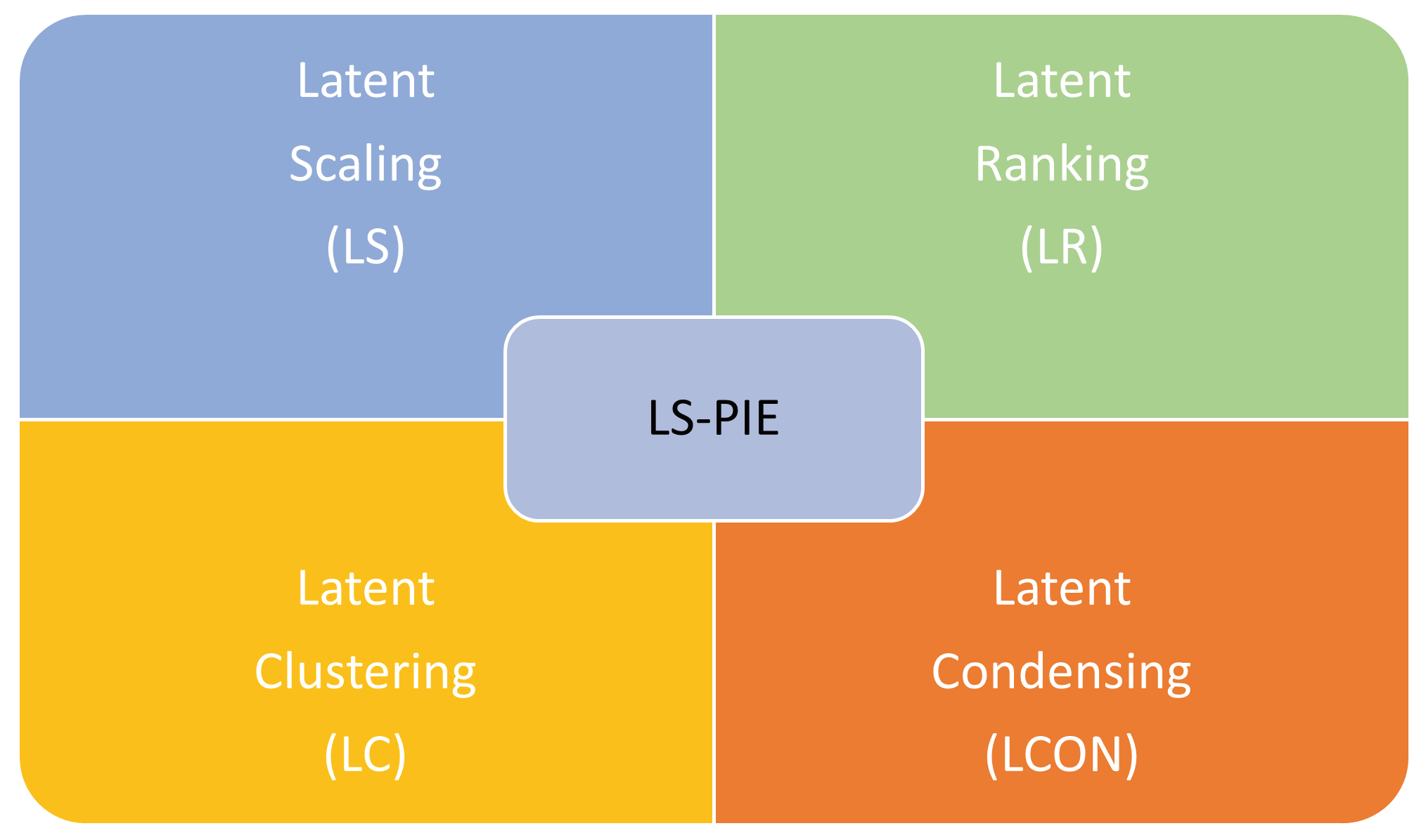
5.1. Latent Scaling (LS)

Latent scaling (LS) allows the user to specify a metric to scale the length of latent vectors, e.g., variance. This enhances the visual interpretation of latent vectors when plotted to interrogate them critically. The framework supports several metrics but allows for metrics expressed as user-defined Python functions. The LS algorithm is outlined in Algorithm 1.

Algorithm 1 Latent scaling (LS)

Require: Hankelised or multi-channel time-series data matrix $\mathbf{H}$, user-specified number  of components m, latent variable model $LVM$, scaling metric with associated scaling  function $\mathcal{S}(\mathbf{L},\mathbf{s})$ Ensure: Returns scaled latent components ${\mathbf{L}}_{scaled}$.  1: $\mathbf{L}\leftarrow LVM(\mathbf{H},m)$               ▹ Decompose $\mathbf{H}$ into m latent vectors  2: ${\mathbf{L}}_{scaled}\leftarrow \{\mathcal{S}({\mathbf{L}}_j,s_j)\mid j=1,2,\cdots ,m\}=\{s_1{\mathbf{L}}_1,s_2{\mathbf{L}}_2,...,s_m{\mathbf{L}}_m\}$ ▹ Scale each latent component  return ${\mathbf{L}}_{scaled}$  Scaling Function $\mathcal{S}$($\mathbf{L}$, ${\mathbf{s}}_i\left(\mathbf{L}\right)$):  0. Identity: ${\mathbf{s}}_0\left(\mathbf{L}\right)=\mathbf{I}=\mathbf{L}$            ▹ Keeps original vector unchanged  1. Variance: ${\mathbf{s}}_1\left(\mathbf{L}\right)=\left[\mathrm{Var}\left({\mathbf{L}}_{\mathbf{j}}\right)\right],j=1,\cdots ,k$  2. Kurtosis: ${\mathbf{s}}_2\left(\mathbf{L}\right)=\left[\mathrm{Kurt}\left({\mathbf{L}}_j\right)\right],j=1,\cdots ,k$  3. Spectral centroid: ${\mathbf{s}}_3\left(\mathbf{L}\right)={\displaystyle \frac{{\sum }_{j=0}^{N/2}(j·\frac{f_s}{N})·\left|\mathrm{FFT}{\left(\mathbf{L}\right)}_j\right|}{{\sum }_{j=0}^{N/2}\left|\mathrm{FFT}{\left(\mathbf{L}\right)}_j\right|}}$  4. Entropy: ${\mathbf{s}}_4\left({\mathbf{L}}_{\mathbf{j}}\right)=-{\sum }_k{p}_{k}log{p}_k$, with $p_k$ the probability of the k-th element in ${\mathbf{L}}_j$

This allows for the scaling of each latent direction based on the scaling score. Scaling scores include variance and kurtosis. Variance allows us to highlight latent directions that are prominent in reconstruction while hiding latent directions that do not contribute significantly to reconstruction, while kurtosis is a proxy for identifying potential variance sources [4].

5.2. Latent Ranking (LR)

Latent ranking (LR) allows the user to specify a feature metric and then rank the latent variables according to the selected feature metric. Although several feature metrics are readily available, the framework allows for a feature metric specified as a user-defined Python function. The LR algorithm is outlined in Algorithm 2.

Algorithm 2 Latent ranking (LR)

Require: Hankelised or multi-channel time-series data matrix $\mathbf{H}$, latent variable model  $LVM$, user-specified number of latent components m, user-selected or user-specified  feature mapping function f. Ensure: Returns ranked latent components ${\mathbf{L}}_{ranked}$ and the ranked feature scores ${\mathbf{f}}_{ranked}$.  1: $\mathbf{L}\leftarrow LVM(\mathbf{H},m)$              ▹ Decompose $\mathbf{H}$ into m latent vectors  2: $\mathbf{f}\leftarrow f\left(\mathbf{L}\right)$;                ▹ Map latent vectors to a feature space  3: ${\mathbf{L}}_{ranked},{\mathbf{f}}_{ranked}\leftarrow sort(\mathbf{L},\mathbf{f})$ ▹ sort the latent vectors according to their features scores  return ${\mathbf{L}}_{ranked},{\mathbf{f}}_{ranked}$  Feature mapping function f:  1. Variance: $f_1\left(\mathbf{L}\right)=\left[\mathrm{Var}\left({\mathbf{L}}_{\mathbf{j}}\right)\right],j=1,\cdots ,k$  2. Kurtosis: $f_2\left(\mathbf{L}\right)=\left[\mathrm{Kurt}\left({\mathbf{L}}_j\right)\right],j=1,\cdots ,k$  3. Spectral centroid: $f_3\left(\mathbf{L}\right)={\displaystyle \frac{{\sum }_{j=0}^{N/2}(j·\frac{f_s}{N})·\left|\mathrm{FFT}{\left(\mathbf{L}\right)}_j\right|}{{\sum }_{j=0}^{N/2}\left|\mathrm{FFT}{\left(\mathbf{L}\right)}_j\right|}}$  4. Entropy: $f_4\left({\mathbf{L}}_{\mathbf{j}}\right)=-{\sum }_k{p}_{k}log{p}_k$, where $p_k$ is the probability of the k-th element in ${\mathbf{L}}_j$

Latent ranking allows for exploring latent variables that have already been identified by optimising some regularised optimisation problem. It also enables unordered latent variables to be ordered or allows us to order latent variables according to some other metric than what the LVM used to extract latent components, which could enhance the interpretation of the current latent variables, exploring some of their underlying characteristics.

5.3. Latent Clustering (LC)

We also need to counter an additional common problem in some LVMs. Unlike PCA, where the number of components increases, existing components remain unchanged, and new components explain less and less variance. Some LVMs split the same information over more and more components as the number of latent directions increases, e.g., ICA. Latent clustering combines similar latent directions according to a user-defined metric into a single latent direction through clustering.

For linear models, the maximum number of latent dimensions is dictated by the rank of the data matrix $\mathbf{X}$ after standardisation. Latent clustering (LC) enables the user to specify the number of latent clusters to be identified from the specified number of latent variables, i.e., LC clusters latent directions into a pre-selected number of clusters. LC can be performed by selecting available similarity or dissimilarity metrics or as a user-specified Python function, and the clustering approach with BIRCH is the default for LC. The algorithmic implementation of this approach is given in Algorithm 3.

Algorithm 3 Latent clustering (LC)

Require: Hankelised or multi-channel time-series data matrix $\mathbf{H}$, latent variable model  $LVM$, clustering algorithm C, feature mapping function f, distance metric d, cluster  scoring function s, specified or maximum number of latent vectors m, specified number  of latent clusters k. Ensure: For k clusters find the feature clustering ${\mathbf{R}}_k$, cluster score $S_k$ and latent cluster  components ${\mathbf{L}}_k$  1: $\mathbf{L}\leftarrow LVM(\mathbf{H},m)$               ▹ Decompose $\mathbf{H}$ into m latent vectors  2: $\tilde{\mathbf{F}}\leftarrow f\left(\mathbf{L}\right)$                  ▹ Map latent vectors to feature space  3: $\mathbf{F}\leftarrow scale\left(\tilde{\mathbf{F}}\right)$                ▹ User-specified feature space scaling  4: ${\mathbf{R}}_k,{\mathbf{L}}_k\leftarrow C(\mathbf{F},d,\mathbf{L},k)$        ▹ Cluster into k clusters using distance metric d  5: $S_k\leftarrow s({\mathbf{R}}_k,{\mathbf{L}}_k,\mathbf{H})$                       ▹ Cluster scoring     return ${\mathbf{R}}_k$, ${\mathbf{L}}_k$, $S_k$     Feature Mapping Function f:  $f\left(\mathbf{L}\right)=\left[f_i\right]$, where $f_i$ are selected individual feature functions that could include:  0. Identity: $\mathbf{I}\mathbf{L}=\mathbf{L}$               ▹ Keeps original vector unchanged  1. Variance: $f_1\left(\mathbf{L}\right)=\left[\mathrm{Var}\left({\mathbf{L}}_{\mathbf{j}}\right)\right],j=1,\cdots ,k$  2. Kurtosis: $f_2\left(\mathbf{L}\right)=\left[\mathrm{Kurt}\left({\mathbf{L}}_j\right)\right],j=1,\cdots ,k$  3. Spectral centroid: $f_3\left(\mathbf{L}\right)={\displaystyle \frac{{\sum }_{j=0}^{N/2}(j·\frac{f_s}{N})·\left|\mathrm{FFT}{\left(\mathbf{L}\right)}_j\right|}{{\sum }_{j=0}^{N/2}\left|\mathrm{FFT}{\left(\mathbf{L}\right)}_j\right|}}$  4. Entropy: $f_4\left({\mathbf{L}}_{\mathbf{j}}\right)=-{\sum }_k{p}_{k}log{p}_k$, with $p_k$ the probability of the k-th element in ${\mathbf{L}}_j$    Distance metrics d for clustering:  - Euclidean distance: $d(\mathbf{x},\mathbf{y})={\parallel \mathbf{x}-\mathbf{y}\parallel }_2$ [42]  - Manhattan distance: $d(\mathbf{x},\mathbf{y})={\parallel \mathbf{x}-\mathbf{y}\parallel }_1$ [43]  - Cosine distance: $d(\mathbf{x},\mathbf{y})=1-{\displaystyle \frac{\mathbf{x}·\mathbf{y}}{{\parallel \mathbf{x}\parallel }_2{\parallel \mathbf{y}\parallel }_2}}$ [44]  - Mahalanobis distance: $d(\mathbf{x},\mathbf{y})=\sqrt{{(\mathbf{x}-\mathbf{y})}^T{\mathbf{S}}^{-1}(\mathbf{x}-\mathbf{y})}$, where $\mathbf{S}$ is the covariance matrix [45]    Cluster scoring functions s:  1. Silhouette score: $s(\mathbf{R},\mathbf{L},\mathbf{H})={\displaystyle \frac{1}{\left|\mathbf{L}\right|}}{\sum }_{{\mathbf{L}}_j\in \mathbf{L}}{\displaystyle \frac{b\left({\mathbf{L}}_{\mathbf{j}}\right)-a\left({\mathbf{L}}_{\mathbf{j}}\right)}{max(a\left({\mathbf{L}}_{\mathbf{j}}\right),b\left({\mathbf{L}}_{\mathbf{j}}\right))}}$  $a\left({\mathbf{L}}_{\mathbf{j}}\right)$ is the mean intra-cluster distance, and $b\left({\mathbf{L}}_{\mathbf{j}}\right)$ is the mean nearest-cluster distance  2. Variance-based: $s(\mathbf{R},\mathbf{L},\mathbf{H})={\displaystyle \frac{1}{\left|\mathbf{L}\right|}}{\displaystyle \frac{\mathrm{tr}\left({\mathbf{L}}^T{\mathbf{H}}^T\mathbf{H}\mathbf{L}\right)}{\mathrm{tr}\left({\mathbf{H}}^T\mathbf{H}\right)}}$  3. Kurtosis-based: $s(\mathbf{R},\mathbf{L},\mathbf{H})={\displaystyle \frac{1}{\left|\mathbf{L}\right|}}{\sum }_{j=1}^{\left|\mathbf{L}\right|}\left|\mathrm{Kurt}\left({\mathbf{L}}_j^{\mathrm{T}}{\mathbf{H}}^{\mathrm{T}}\right)\right|$  4. Frequency-based: $s(\mathbf{R},\mathbf{L},\mathbf{H})={\displaystyle \frac{1}{\left|\mathbf{L}\right|}}{\sum }_{j=1}^{\left|\mathbf{L}\right|}{\displaystyle \frac{{\sum }_k{(f_k-{\mu }_j)}^2\left|\mathrm{FFT}{\left(\left({\mathbf{L}}_j^T{\mathbf{H}}^{\mathrm{T}}\right)\right)}_k\right|}{{\sum }_k\left|\mathrm{FFT}{\left(\left({\mathbf{L}}_j^T{\mathbf{H}}^{\mathrm{T}}\right)\right)}_k\right|}}$

5.4. Latent Condensing (LCON)

Latent condensing allows optimal latent discovery by extending LC to automatically estimate the optimal latent dimensions and directions using selected clustering algorithms and approaches. While LC finds a user-prescribed number of components/clusters, LCON aims to automate dimensionality reduction utilising two main strategies:

• Systematically reducing the latent dimensions solved by the algorithm and minimising or maximising a selected clustering index to find the optimal number of clusters.
• Utilising algorithmic clustering to find the optimal number of latent clusters such as balanced iterative reducing and clustering using hierarchies (BIRCH) [46] or density-based spatial clustering of applications with noise (DBSCAN) [47,48].

From Algorithm 4, we can see that for both cases, we first transform the input data into the maximal number of components using an LVM, in this case, FastICA. We then utilise a feature-mapping function to map these components to a features space, in these examples, explained variance. We then manually reduce the number of components to be solved and repeat the process in regular increments, with the most thorough being to decrease by 1 component each time. Alternatively, we utilise an automated approach, such as clustering algorithms, to compress the latent space. In this case, we use a selective clustering algorithm to automatically identify the optimal number of latent components within the feature space. Unlike other methods, LCON takes the raw input matrix, in our case, Hankelised time data, as its input and utilises the choice of LVM at each step in the process. The algorithmic implementation is shown in Algorithm 4. In this paper, we use DBSCAN as the default for LCON. This shows the potential to fully automate the algorithm, as with PCA, to allow for simpler application of analytical tools. In this case, the ability of algorithms such as DBSCAN to automatically find the number of clusters removes the need for user-specified component numbers instead of relying on the user to specify them.

Algorithm 4 Latent condensing (LCON) for Hankelised time-series data

Require: Hankelised or multi-channel time-series data matrix $\mathbf{H}$, latent variable model  $LVM$, clustering algorithm C, feature mapping function f, distance metric d, cluster  scoring function s, specified or maximum number of latent vectors m, clustering  approach $Automatic$ or not Ensure: Best feature clustering ${\mathbf{R}}_{best}$, cluster score $S_{best}$ and latent cluster components ${\mathbf{L}}_{best}$  1: $S_{best}\leftarrow -\infty$  2: ${\mathbf{R}}_{best}\leftarrow \varnothing$  3: for$k\leftarrow m$ to 1 do  4:     $\mathbf{L}\leftarrow LVM(\mathbf{H},k)$               ▹ Decompose $\mathbf{H}$ into k latent vectors  5:     $\tilde{\mathbf{F}}\leftarrow f\left(\mathbf{L}\right)$                 ▹ Map latent vectors to feature space  6:     $\mathbf{F}\leftarrow scale\left(\tilde{\mathbf{F}}\right)$               ▹ User-specified feature space scaling  7:     if Automatic then  8:         ${\mathbf{R}}_{auto},{\mathbf{L}}_{auto}\leftarrow C(\mathbf{F},d,\mathbf{L})$        ▹ Automatic feature clustering ${\mathbf{R}}_{auto}$ using  user-specified distance metric d to find protype latent vectors ${\mathbf{L}}_{auto}$  9:         $S_{auto}\leftarrow s({\mathbf{R}}_{auto},{\mathbf{L}}_{auto})$                    ▹ Cluster scoring 10:         if $S_{auto}>S_{best}$ then 11:            $S_{best}\leftarrow S_{auto}$ 12:            ${\mathbf{R}}_{best}\leftarrow {\mathbf{R}}_{auto}$ 13:            ${\mathbf{L}}_{best}\leftarrow {\mathbf{L}}_{auto}$ 14:         end if 15:     else 16:         for $j\leftarrow k$ to 1 do 17:            ${\mathbf{R}}_j,{\mathbf{L}}_j\leftarrow C(\mathbf{F},d,\mathbf{L},j)$     ▹ Cluster into j clusters using distance metric d 18:            $S_j\leftarrow s({\mathbf{R}}_j,{\mathbf{L}}_j,\mathbf{H})$                    ▹ Cluster scoring 19:            if $S_j>S_{best}$ then 20:                $S_{best}\leftarrow S_j$ 21:                ${\mathbf{R}}_{best}\leftarrow {\mathbf{R}}_j$ 22:                ${\mathbf{L}}_{best}\leftarrow {\mathbf{L}}_j$ 23:            end if 24:         end for 25:     end if 26: end for     return ${\mathbf{R}}_{best}$, ${\mathbf{L}}_{best}$, $S_{best}$  Feature mapping function f:  $f\left(\mathbf{L}\right)=\left[f_i\right]$, where $f_i$ are selected individual feature functions that could include:  0. Identity: $\mathbf{I}\mathbf{L}=\mathbf{L}$              ▹ Keeps original vector unchanged  1. Variance: $f_1\left(\mathbf{L}\right)=\left[\mathrm{Var}\left({\mathbf{L}}_{\mathbf{j}}\right)\right],j=1,\cdots ,k$  2. Kurtosis: $f_2\left(\mathbf{L}\right)=\left[\mathrm{Kurt}\left({\mathbf{L}}_j\right)\right],j=1,\cdots ,k$  3. Spectral centroid: $f_3\left(\mathbf{L}\right)={\displaystyle \frac{{\sum }_{j=0}^{N/2}(j·\frac{f_s}{N})·\left|\mathrm{FFT}{\left(\mathbf{L}\right)}_j\right|}{{\sum }_{j=0}^{N/2}\left|\mathrm{FFT}{\left(\mathbf{L}\right)}_j\right|}}$  4. Entropy: $f_4\left({\mathbf{L}}_{\mathbf{j}}\right)=-{\sum }_k{p}_{k}log{p}_k$, with $p_k$ the probability of the k-th element in ${\mathbf{L}}_j$  Distance metrics d for clustering:  1. Euclidean distance: $d(\mathbf{x},\mathbf{y})={\parallel \mathbf{x}-\mathbf{y}\parallel }_2$ [42]  2. Manhattan distance: $d(\mathbf{x},\mathbf{y})={\parallel \mathbf{x}-\mathbf{y}\parallel }_1$ [43]  3. Cosine distance: $d(\mathbf{x},\mathbf{y})=1-{\displaystyle \frac{\mathbf{x}·\mathbf{y}}{{\parallel \mathbf{x}\parallel }_2{\parallel \mathbf{y}\parallel }_2}}$ [44]  4. Mahalanobis distance: $d(\mathbf{x},\mathbf{y})=\sqrt{{(\mathbf{x}-\mathbf{y})}^T{\mathbf{S}}^{-1}(\mathbf{x}-\mathbf{y})}$, where $\mathbf{S}$ is the covariance matrix [45]  Cluster scoring functions s:  1. Silhouette score: $s(\mathbf{R},\mathbf{L},\mathbf{H})={\displaystyle \frac{1}{\left|\mathbf{L}\right|}}{\sum }_{{\mathbf{L}}_j\in \mathbf{L}}{\displaystyle \frac{b\left({\mathbf{L}}_{\mathbf{j}}\right)-a\left({\mathbf{L}}_{\mathbf{j}}\right)}{max(a\left({\mathbf{L}}_{\mathbf{j}}\right),b\left({\mathbf{L}}_{\mathbf{j}}\right))}}$  $a\left({\mathbf{L}}_{\mathbf{j}}\right)$ is the mean intra-cluster distance, and $b\left({\mathbf{L}}_{\mathbf{j}}\right)$ is the mean nearest-cluster distance  2. Variance-based: $s(\mathbf{R},\mathbf{L},\mathbf{H})={\displaystyle \frac{1}{\left|\mathbf{L}\right|}}{\displaystyle \frac{\mathrm{tr}\left({\mathbf{L}}^T{\mathbf{H}}^T\mathbf{H}\mathbf{L}\right)}{\mathrm{tr}\left({\mathbf{H}}^T\mathbf{H}\right)}}$  3. Kurtosis-based: $s(\mathbf{R},\mathbf{L},\mathbf{H})={\displaystyle \frac{1}{\left|\mathbf{L}\right|}}{\sum }_{j=1}^{\left|\mathbf{L}\right|}\left|\mathrm{Kurt}\left({\mathbf{L}}_j^{\mathrm{T}}{\mathbf{H}}^{\mathrm{T}}\right)\right|$  4. Frequency-based: $s(\mathbf{R},\mathbf{L},\mathbf{H})={\displaystyle \frac{1}{\left|\mathbf{L}\right|}}{\sum }_{j=1}^{\left|\mathbf{L}\right|}{\displaystyle \frac{{\sum }_k{(f_k-{\mu }_j)}^2\left|\mathrm{FFT}{\left(\left({\mathbf{L}}_j^T{\mathbf{H}}^{\mathrm{T}}\right)\right)}_k\right|}{{\sum }_k\left|\mathrm{FFT}{\left(\left({\mathbf{L}}_j^T{\mathbf{H}}^{\mathrm{T}}\right)\right)}_k\right|}}$  ${\mu }_j$ is the mean frequency for the j-th latent component

6. Numerical Investigation

The effectiveness of LR, LS, and LCON is showcased using two crafted foundational problems using single-channel data. In both cases, Hankelisation is employed before applying two latent variable models: PCA and ICA.

6.1. Single Channel: Latent Ranking (LR), Latent Scaling (LS), and Latent Condensing (LCON)

To show the effects of the LS-PIE module on the generated latent spaces, we consider a foundational example

$$f\left(t\right)=sin\left(2\pi t\right)$$

uniformly sampled at ${\displaystyle \frac{4000}{12\pi }}$ samples per second using Hankelisation with a window length of 300. The results for extracting eight latent variables using PCA and ICA are shown in Figure 4. Here, we expect identical results for PCA and ICA, merely a single-frequency Fourier sin-cosine decomposition, as shown in Figure 5. Note the improvement in informativeness as latent scaling (LS) is applied. In turn, note the improvement in the informativeness of the latent directions of latent ranking (LR) and enhancement of latent condensing (LC) for ICA. For ICA, LC combines the second- and third-ranked ICs.

In turn, Figure 4 is a signal with decreasing frequency over time, expressed by $f\left(t\right)=sin\left(2\pi t^{0.85}\right)$. Here, we expect to see some differentiation in the latent directions between PCA and ICA, as shown in Figure 6. The improvement in interpretation and informativeness of the latent directions using LS-PIE is evident. LS-PIE isolates and enhances the essential latent directions that allow time for the critical interpretation of latent directions and the comparison between LVMs.

6.2. Multi-Channel Real World Data

6.2.1. Background

To showcase the application of the module on real-world, multi-channel data, we apply the module on a compiled ECG Heartbeat Categorisation Dataset. This dataset consists of 14552 samples at 125Hz, all falling within two categories: healthy and unhealthy. We can treat the total system as an input matrix because we have multiple examples of vector signals. This means we do not need to transform the input data before analysing it.

This dataset is used to train deep neural networks [49]. However, each of these samples is of a very high dimension, consisting of 188 data points requiring larger deep neural networks to analyse.

The data are available through PhysioNet as a combination of the MIT-BIH Arrhythmia Database and the PTB Diagnostic ECG Database.

6.2.2. Analysis

We apply LS, LR, LC, and LCON. In this case, we do not have to re-shape our input data before applying the LVM to the data, thereby investigating FastICA before and after applying LR, LS, LC, and LCON.

By comparing Figure 7 and Figure 8 we can see that the two approaches condense the input data differently. In this case the ranking approach showcased in Figure 7 allows for clear differentiation between classes whereas from Figure 8, we can see that the clustering functionality overly compensates for noise in the data, gathering all meaningful information into a single signal while returning two noise signals. This means the statistically significant distribution generated by the ranked LS-PIE functionality is absent in the clustered signals.

6.2.3. Comparison of Results

This section clearly shows the improvements added using the LS-PIE functionality to improve the analysis of large datasets. From Figure 9, we can see an even clearer representation of the difference between the two data classes. In the case of noisy, less linear data, the ranking functionality separated clear differences in magnitude between the two data types, whereas the clustered method overcompensated, forcing all the information into one meaningless vector. However, both contain more information than undirected FastICA decomposition; in this case, the components were over-decomposed, and the information was lost to random noise.

6.3. Discussion

These two experimental analyses show the improvements of the latent representations generated using FastICA. For simple sinusoidal problems, we can see that the ranked and scaled FastICA results more closely resemble the recovered PCA results. Additionally, we can see that before applying LR and LS, the components seemingly showed random noise. This noise complicates the informed analysis of the datasets.

These results are clearer when we examine the ranked and scaled decomposition of the ECG dataset provided in Figure 7. In this case, clear differences in the distributions of the latent variables can be seen. This would allow this method to be used to pre-process data for categorisation. However, this example also highlights the specific applicability of the two approaches. For this dataset, the LC and LCON methods could not recover significantly different results when applied to the normal and abnormal heartbeat datasets.

6.4. Discussion of Use Cases

From these two example datasets, we can see that the latent ranking, latent scaling, latent clustering, and latent condensing methods described within this paper function best when applied in tandem, allowing for maximally interpretable latent spaces. Figure 7 shows that we recover far more interpretable data when latent components are ranked and scaled. Applying these two approaches allows us to organise latent components for ICA in a way that is similar to PCA.

7. Impact

The role of LS-PIE in interrogating LVMs and enhancing latent directions is demonstrated in two foundational example problems. LS-PIE ensures that the user can focus their time and energy on interpreting the latent space for latent inference instead of first defining an informative latent space. The potential impact of LS-PIE is an improved adoption of interpretation-centred LVMs in signal processing, vibration-based condition monitoring, actuarial sciences, finances, and social and physical sciences, as well as the enhanced interpretation of reconstruction-centred LVMs.

The application of ranking, scaling, clustering, and condensing is showcased for artificially generated and real-world ECG data. In these cases, we can see that the clustering approach allows the number of components to be extracted from larger datasets. In contrast, the ranking approach works well to generate interpretable latent spaces, as shown in the clear difference in results in the multi-channel section.

These approaches allow for the use of a wider array of LVMs as pre-processing methods for further data analysis.

This initial LS-PIE framework is a latent variable ecosystem to enhance the practical application of LVMs, centring research activity of LVMs around latent inference for interpretation.

8. Conclusions

LS-PIE improves the interpretability of reconstruction- and interpretation-centred LVMs through latent ranking and scaling while enhancing the information spread over latent directions through latent condensing. Two foundational datasets highlight the benefit of utilising LS-PIE to improve the informativeness for reconstruction-centred and interpretation-centred LVMs. Additionally, the ECG dataset shows that the methods can be applied in tandem to allow for more meaningful analysis of real-world datasets.

From the two foundational examples we can see a reduction of noise and improvement of latent clarity in the two example problems analysed. We can see that for simple linear problems, the LS-PIE approach is able to direct the undirected latent space of the FastICA algorithm and extract more interpretable components. This can be seen in Figure 5. The experimental analysis in Section 6.2 further showcases the improvements derived from the application of LS-PIE. From Figure 7 and Figure 9, it can be seen that simple LVMs augmented with LS-PIE are capable of compressing higher dimensional, complex data into far more compact linear representations while still retaining informative characteristics and allowing for more educated further analysis.

The LS-PIE framework is the first step towards an LVM ecosystem that benefits the practical application and research opportunities of LVMs. Future research will develop additional functionality that benefits LVM research and the practical deployment of LVM for industrial applications.

The main conclusions and innovations presented in this paper can be summarised as follows:

• LS-PIE is applicable to source- and reconstruction-focused LVMs;
• It returns interpretable components;

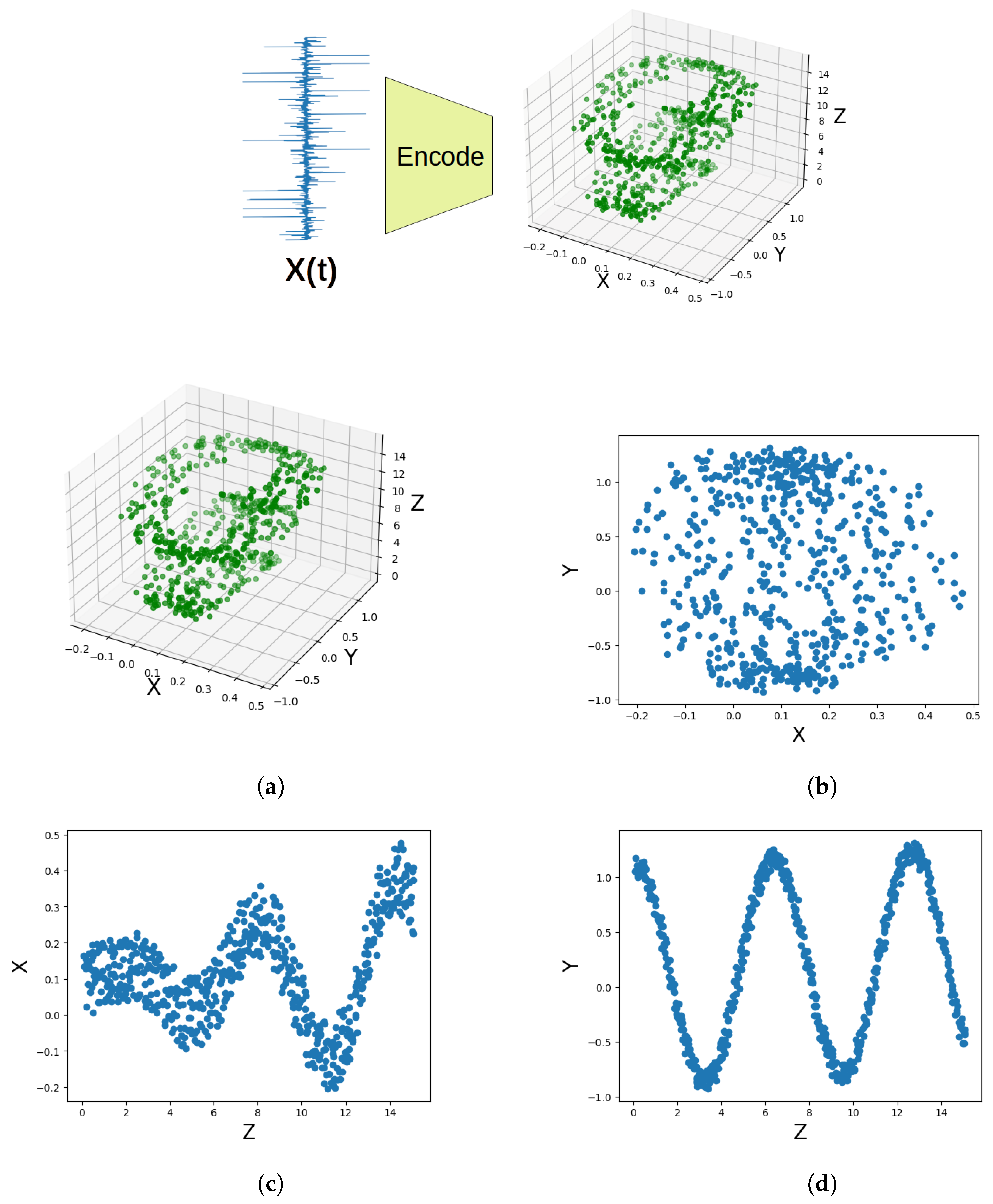
  (a)

  Ranking and scaling help to organize latent spaces;

  (b)

  Clustering and condensing help solve for optimal representations;

• The approach is applicable to both artificial and real-world data;

  (a)

  In both cases, it improves the latent interpretability;

  (b)

  The real-world data showcase their applicability as pre-processing metrics;

• The algorithm is designed to be fully customisable to a users requirements.

9. Future Work

The LS-PIE algorithm can further be improved by automating the extraction of components. Many LVMs, such as PCAs, extract maximal components in descending order of variance. This means that as the number of components increases, a point is reached where nearly all of the variance has been explained. Beyond this, further components have a magnitude of zero. However, others, such as FastICA, split sources to create more components, slowly reducing the information in any given component.

To counteract this, we can find the optimal number of latent clusters using LCON. LCON achieves this by selective clustering algorithms that identify the optimal number of clusters or by iterating from two to the maximum number of clusters until a user-specified metric is met, e.g., the maximum variance per component.

Further research is required in order to evaluate the scalability of these methods as well as the impact of choice of analysis metrics and LVM on the generated results. The authors hope to conduct a more in depth study comparing the results of further classes of latent variable models on a wider range of data. Additionally, further work will aim to apply the LS-PIE algorithms to a wider range of models, such as PCA and ICA variants, e.g., CCA and disjoint PCA, as well as approaches such as Group ICA or kernal ICA and more complex N-Way models such as PARAFAC and Tucker3.

References

1. Booyse, W.; Wilke, D.N.; Heyns, S. Deep digital twins for detection, diagnostics and prognostics. Mech. Syst. Signal Process. 2020, 140, 106612. [Google Scholar] [CrossRef]
2. Wilke, D.N. Digital Twins for Physical Asset Lifecycle Management. In Digital Twins: Basics and Applications; Lv, Z., Fersman, E., Eds.; Springer International Publishing: Cham, Switzerland, 2022; pp. 13–26. [Google Scholar] [CrossRef]
3. Wilke, D.N. Lecture Notes in Optimum Design for Information Extraction from Data: Mastering Unsupervised Learning; Department of Mechanical and Aeronautical Engineering, Univerrsity of Pretoria: Pretoria, South Africa, 2021. [Google Scholar]
4. Wilke, D.N.; Heyns, P.S.; Schmidt, S. The Role of Untangled Latent Spaces in Unsupervised Learning Applied to Condition-Based Maintenance. In Modelling and Simulation of Complex Systems for Sustainable Energy Efficiency; Hammami, A., Heyns, P.S., Schmidt, S., Chaari, F., Abbes, M.S., Haddar, M., Eds.; Springer: Cham, Switzerland, 2022; pp. 38–49. [Google Scholar] [CrossRef]
5. Lever, J.; Krzywinski, M.; Altman, N. Points of Significance: Principal component analysis. Nat. Methods 2017, 14, 641–642. [Google Scholar] [CrossRef]
6. Jaadi, Z.; Powers, J.; Pierre, S. Principal Component Analysis (PCA) Explained; Built In: Chicago, IL, USA, 2022. [Google Scholar]
7. Golyandina, N.; Zhigljavsky, A. Singular Spectrum Analysis for Time Series; Springer: Berlin/Heidelberg, Germany, 2013. [Google Scholar] [CrossRef]
8. Wilke, D.N.; Schmidt, S.; Heyns, P.S. A Review of Singular Spectral Analysis to Extract Components from Gearbox Data. In International Workshop on Modelling and Simulation of Complex Systems for Sustainable Energy Efficiency; Applied Condition Monitoring; Springer: Cham, Switzerland, 2021; Volume 20, pp. 160–172. [Google Scholar]
9. Tharwat, A. Independent component analysis: An introduction. Appl. Comput. Inform. 2018, 17, 222–249. [Google Scholar] [CrossRef]
10. De Lathauwer, L.; De Moor, B.; Vandewalle, J. An introduction to independent component analysis. J. Chemom. 2000, 14, 123–149. [Google Scholar] [CrossRef]
11. Hyvärinen, A.; Karhunen, J.; Oja, E. What is Independent Component Analysis? In Independent Component Analysis; John Wiley & Sons, Ltd.: Hoboken, NJ, USA, 2001; Chapter 7; pp. 145–164. [Google Scholar] [CrossRef]
12. Westad, F. Independent component analysis and regression applied on sensory data. J. Chemom. 2005, 19, 171–179. [Google Scholar] [CrossRef]
13. Kohonen, T. An adaptive associative memory principle. IEEE Trans. Comput. 1974, 100, 444–445. [Google Scholar] [CrossRef]
14. Rumelhart, D.E.; Hinton, G.E.; Williams, R.J. Learning representations by back-propagating errors. Nature 1986, 323, 533–536. [Google Scholar] [CrossRef]
15. Snyman, J.A.; Wilke, D.N. Practical Mathematical Optimization, 2nd ed.; Springer Optimization and Its Applications; Springer: Cham, Switzerland, 2018; pp. XXVI+372. [Google Scholar] [CrossRef]
16. Marino, J.; Chen, L.; He, J.; Mandt, S. Improving sequential latent variable models with autoregressive flows. Mach. Learn. 2022, 111, 1597–1620. [Google Scholar] [CrossRef]
17. Liu, Y.; Zheng, C. Deep latent variable models for generating knockoffs. Stat 2019, 8, e260. [Google Scholar] [CrossRef]
18. Candes, E.; Fan, Y.; Janson, L.; Lv, J. Panning for Gold: Model-X Knockoffs for High-dimensional Controlled Variable Selection. arXiv 2016, arXiv:1610.02351. [Google Scholar] [CrossRef]
19. Chandra, R.; Jain, M.; Maharana, M.; Krivitsky, P.N. Revisiting Bayesian Autoencoders With MCMC. IEEE Access 2022, 10, 40482–40495. [Google Scholar] [CrossRef]
20. Song, G.; Wang, S.; Huang, Q.; Tian, Q. Harmonized Multimodal Learning with Gaussian Process Latent Variable Models. IEEE Trans. Pattern Anal. Mach. Intell. 2021, 43, 858–872. [Google Scholar] [CrossRef] [PubMed]
21. Kong, X.; Jiang, X.; Zhang, B.; Yuan, J.; Ge, Z. Latent variable models in the era of industrial big data: Extension and beyond. Annu. Rev. Control 2022, 54, 167–199. [Google Scholar] [CrossRef]
22. Golyandina, N.; Dudnik, P.; Shlemov, A. Intelligent Identification of Trend Components in Singular Spectrum Analysis. Algorithms 2023, 16, 353. [Google Scholar] [CrossRef]
23. Wadekar, S.; Mahalkari, A.; Ali, A.; Gupta, A. Abstract Proceedings of International Conference on 2022 IEEE International Conference on Current Development in Engineering and Technology (CCET): 23rd–24th December 2022; IEEE: Piscataway, NJ, USA, 2022. [Google Scholar] [CrossRef]
24. Karhunen, J.; Honkela, A.; Raiko, T.; Harva, M.; Ilin, A.; Tornio, M.; Valpola, H. Bayesian Learning of Latent Variable Models. Available online: https://users.ics.aalto.fi/juha/biennial2007-bayes.pdf (accessed on 31 May 2024).
25. Tucker, L. Some mathematical notes on three-mode factor analysis. Psychometrika 1966, 31, 279–311. [Google Scholar] [CrossRef]
26. Andersson, C.A.; Bro, R. Improving the speed of multi-way algorithms: Part I. Tucker3. Chemom. Intell. Lab. Syst. 1998, 42, 93–103. [Google Scholar] [CrossRef]
27. Gallo, M. Tucker3 Model for Compositional Data. Commun. Stat.-Theory Methods 2015, 44, 4441–4453. [Google Scholar] [CrossRef]
28. Murphy, K.R.; Stedmon, C.A.; Graeber, D.; Bro, R. Fluorescence spectroscopy and multi-way techniques. PARAFAC. Anal. Methods 2013, 5, 6557–6566. [Google Scholar] [CrossRef]
29. Bro, R. Parafac. Tutorial and Applications. Chemom. Intell. Lab. Syst. 1997, 38, 149–191. [Google Scholar] [CrossRef]
30. Bach, F.R.; Jordan, M.I. Kernel independent component analysis. J. Mach. Learn. Res. 2002, 3, 1–48. [Google Scholar] [CrossRef]
31. Cavicchia, C.; Vichi, M.; Zaccaria, G. Hierarchical disjoint principal component analysis. AStA Adv. Stat. Anal. 2023, 107, 537–574. [Google Scholar] [CrossRef]
32. d’Aspremont, A.; Ghaoui, L.E.; Jordan, M.I.; Lanckriet, G.R. A direct formulation for sparse PCA using semidefinite programming. SIAM Rev. 2007, 49, 434–448. [Google Scholar] [CrossRef]
33. Bertsimas, D.; Cory-Wright, R.; Pauphilet, J. Solving Large-Scale Sparse PCA to Certifiable (Near) Optimality. arXiv 2020, arXiv:2005.05195. [Google Scholar]
34. Lamboy, W.F. Disjoint Principal Component Analysis: A Statistical Method of Botanical Identification. Source Syst. Bot. 1990, 15, 3–12. [Google Scholar] [CrossRef]
35. Hyvärinen, A. Independent component analysis: Recent advances. Philos. Trans. Math. Phys. Eng. Sci. 2013, 371, 20110534. [Google Scholar] [CrossRef] [PubMed]
36. Broomhead, D.; King, G.P. Extracting qualitative dynamics from experimental data. Phys. D Nonlinear Phenom. 1986, 20, 217–236. [Google Scholar] [CrossRef]
37. Setshedi, I.I.; Loveday, P.W.; Long, C.S.; Wilke, D.N. Estimation of rail properties using semi-analytical finite element models and guided wave ultrasound measurements. Ultrasonics 2019, 96, 240–252. [Google Scholar] [CrossRef]
38. Bach, F.R.; Jordan, M.I. Finding Clusters in Independent Component Analysis. In Proceedings of the 4th International Symposium on Independent Component Analysis and Signal Separation, Nara, Japan, 1–4 April 2003. [Google Scholar]
39. Widom, H.; Society, A.M. Hankel Matrices. Trans. Am. Math. Soc. 1966, 121, 1–35. [Google Scholar] [CrossRef]
40. Yao, F.; Coquery, J.; Lê Cao, K.A. Independent Principal Component Analysis for biologically meaningful dimension reduction of large biological data sets. BMC Bioinform. 2012, 13, 24. [Google Scholar] [CrossRef]
41. Zhao, X.; Ye, B. Similarity of signal processing effect between Hankel matrix-based SVD and wavelet transform and its mechanism analysis. Mech. Syst. Signal Process. 2009, 23, 1062–1075. [Google Scholar] [CrossRef]
42. Dokmanic, I.; Parhizkar, R.; Ranieri, J.; Vetterli, M. Euclidean Distance Matrices: Essential Theory, Algorithms and Applications. IEEE Signal Process. Mag. 2015, 32, 12–30. [Google Scholar] [CrossRef]
43. Singh, A. K-means with Three different Distance Metrics. Int. J. Comput. Appl. 2013, 67, 8887. [Google Scholar] [CrossRef]
44. Lahitani, A.R.; Permanasari, A.E.; Setiawan, N.A. Cosine similarity to determine similarity measure: Study case in online essay assessment. In Proceedings of the 2016 4th International Conference on Cyber and IT Service Management, Bandung, Indonesia, 26–27 April 2016; pp. 1–6. [Google Scholar] [CrossRef]
45. Ghorbani, H. Mahalanobis Distance and its application for detecting Multivariate Outliers. Facta Univ. Ser. Math. Inform. 2019, 34, 583. [Google Scholar] [CrossRef]
46. Zhang, T.; Ramakrishnan, R.; Livny, M. BIRCH: An efficient data clustering method for very large databases. In Proceedings of the 1996 ACM SIGMOD International Conference on Management of Data, SIGMOD ’96, Montreal, QC, Canada, 4–6 June 1996; ACM: New York, NY, USA, 1996; pp. 103–114. [Google Scholar] [CrossRef]
47. Ester, M.; Kriegel, H.P.; Sander, J.; Xu, X. A Density-Based Algorithm for Discovering Clusters in Large Spatial Databases with Noise. In Proceedings of the 2nd International Conference on Knowledge Discovery and Data Mining (KDD), Portland, OR, USA, 2–4 August 1996; AAAI Press: Washington, DC, USA, 1996; pp. 226–231. [Google Scholar]
48. Schubert, E.; Sander, J.; Ester, M.; Kriegel, H.P.; Xu, X. DBSCAN revisited, revisited: Why and how you should (still) use DBSCAN. ACM Trans. Database Syst. (TODS) 2017, 42, 19. [Google Scholar] [CrossRef]
49. Kachuee, M.; Fazeli, S.; Sarrafzadeh, M. ECG Heartbeat Classification: A Deep Transferable Representation. In Proceedings of the 2018 IEEE International Conference on Healthcare Informatics (ICHI), New York, NY, USA, 4–7 June 2018. [Google Scholar] [CrossRef]
Figure 1. (Top) Encoding of high-dimensional time series into a lower-dimensional latent space. (a) A 3D latent representation in X-Y-Z projected onto the (b) X-Y (c) Z-X (d) Z-Y planes. These projections reveal varied latent structural information for the same data, demonstrating the importance of exploring latent representations in data analysis.
Mca 29 00085 g001
Figure 2. A representation of the four transformations implemented using the LS-PIE framework to analyse datasets more deeply. Latent ranking (LR) and latent scaling (LS) rank and scale latent directions based on user-specified metrics. Latent clustering (LC) groups similar latent directions using clustering with a user-specified number of clusters, while latent condensing (LCON) enables optimal latent discovery by estimating the optimal number of clusters to enhance the interpretability and usability of latent space representations.
Mca 29 00085 g002
Figure 3. The auto-encoding structure is often used in latent variable modelling (LVM). The training stage fits the model on the provided data by learning the weights for encoding and decoding. A higher-dimensional data sample is encoded to a lower-dimensional latent space by encoding. The latent representation can then be decoded to obtain a higher-dimensional reconstruction of the sample from its latent representation through decoding. These models are commonly used in many fields of data science for data compression and reconstruction, while latent inferencing has been gaining traction recently [1,2].
Mca 29 00085 g003
Figure 4. Two example signals, (left) f ( t ) = sin ( 2 π t ) and (right) f ( t ) = sin ( 2 π t 0.85 ) , to illustrate some of the functionality of LS-PIE.
Mca 29 00085 g004
Figure 5. For the time-series signal f ( t ) = sin ( 2 π t ) , depicting (top row) normalised latent directions for PCA (left) and ICA (right) without applying latent ranking (LR) or latent scaling (LS). (middle row) Variance-explained ranked and variance-explained scaled latent directions with PCA (left) and ICA (right). (bottom row) Variance-explained ranked and variance-explained scaled latent directions with latent condensing (LC) for PCA (left) and ICA (right).
Mca 29 00085 g005
Figure 6. For the time-series signal f ( t ) = sin ( 2 π t 0.85 ) , depicting (top row) normalised latent directions for PCA and ICA without applying latent ranking (LR) or latent scaling (LS). (middle row) Variance-explained ranked and variance-explained scaled latent directions for PCA and ICA. (bottom row) Variance-explained ranked and variance-explained scaled latent directions with latent condensing (LC) for PCA and ICA.
Mca 29 00085 g006aMca 29 00085 g006b
Figure 7. Comparison of normal and abnormal multi-channel datasets using fast ICA augmented with LR and LS of the normal (left) and abnormal (right) heartbeat datasets showing a clear difference in the independent component (IC) distributions. The bottom row compares the same two datasets using unranked ICs, showing a distinct lack of interpretability. The transformed signal magnitudes represent the unscored component multiplied by the normalised scoring of the signal.
Mca 29 00085 g007
Figure 8. Comparison of normal and abnormal multi-channel datasets using FastICA augmented with LCON and LC of the normal (left) and abnormal (right) heartbeat datasets showing a clear difference in the IC distributions. The bottom row compares the same two datasets using unranked ICs, showing a distinct lack of interpretability. The transformed signal magnitudes represent the unscored component multiplied by the normalised scoring of the signal.
Mca 29 00085 g008aMca 29 00085 g008b
Figure 9. Comparison of the fast Fourier transformed latent components of the normal heartbeat data (left) and the abnormal heartbeat data (right). The top row showcases the LR components that are scaled using LS, the middle row showcases the CL components, and the bottom row showcases normal FastICA. The transformed signal magnitude represents the unscored component multiplied by the normalised scoring of the signal.
Mca 29 00085 g009aMca 29 00085 g009b
Disclaimer/Publisher’s Note: The statements, opinions and data contained in all publications are solely those of the individual author(s) and contributor(s) and not of MDPI and/or the editor(s). MDPI and/or the editor(s) disclaim responsibility for any injury to people or property resulting from any ideas, methods, instructions or products referred to in the content.