Abstract
This paper proposes a Methodology for Assets Selection in Investment Portfolios (MASIP) focused on creating investment portfolios using heuristic algorithms based on the Markowitz and Sharpe models. MASIP selects and allocates financial assets by applying heuristic methods to accomplish three assignments: (a) Select the stock candidates in an initial portfolio; (b) Forecast the asset values for the short and medium term; and (c) Optimize the investment portfolio by using the Sharpe metric. Once MASIP creates the initial portfolio and forecasts its assets, an optimization process is started in which a set with the best weights determines the participation of each asset. Moreover, a rebalancing process is carried out to enhance the portfolio value. We show that the improvement achieved by MASIP can reach 147% above the SP500 benchmark. We use a dataset of SP500 to compare MASIP with state-of-the-art methods, obtaining superior performance and an outstanding Sharpe Ratio and returns compared to traditional investment approaches. The heuristic algorithms proved effective in asset selection and allocation, and the forecasting process and rebalancing contributed to further improved results.
1. Introduction
In financial asset management and investment decision-making, portfolio creation and optimization represent a fundamental paradigm and essential study area. Building investment portfolios addresses the complex task of allocating limited resources to a diverse range of financial assets, as well as forecasting them [1]. This process requires careful analysis of the risks and returns associated with each asset and understanding their interaction in the context of a diversified portfolio. Optimization involves the search for asset combinations that maximize expected returns or minimize risk, all subject to specific constraints and objectives. Similarly, there are diversification and asset selection methodologies, such as the Markowitz portfolio theory and its extensions, value at risk (VaR) models, and asset allocation strategies [2]. The Markowitz Mean-Variance model, also known as the Modern Portfolio Theory (MPT), is presented in Equations (1)–(4), which is a theoretical framework developed by Harry Markowitz [3]. This study is relevant because it allows portfolio optimization and considers risk-taking based on performance and diversification. This quantitative approach provides an objective framework for making investment decisions and lays the foundations for investment management.
where µi is the expected return of the ith asset, Xi is the relative value invested in the asset i, σij represents the covariance between assets, and E(Xi) is the expected return of the portfolio. Notice that the invested amount is normalized to one in the constraint defined by Equation (3), and no negative investments Xis are permitted according to Equation (4). The decision variables are the expected value E(Xi) and the variance V, and the objectives are to achieve maximum profit and minimum risk.
In the model defined by Equations (1)–(4), the variance V of the portfolio is introduced as a risk measure, which is essential for constructing diversified portfolios. Covariance and correlation are also key elements for good diversification [3]. From the mean-variance model, two objectives must be met: firstly, to maximize the portfolio return and secondly, to minimize the risk. These two objectives become the main difficulty for solving the problem. The Sharpe Ratio (ς) is a popular and straightforward function [4]; ς is commonly used in modern portfolio methods [5,6,7], requiring only the expected value of the portfolio, its volatility, and a reference rate [8]. They are called Sharpe Ratio models and offer several advantages, including the facility to reduce the portfolio evaluation problem from a bi-objective scheme to a mono-objective optimization problem with Equations (5)–(7), thereby focusing solely on maximizing the ς function.
where the function indicates the expected differential return per unit of risk associated with different assets conforming to the portfolio, and is the return on a benchmark or the risk-free rate. This portfolio optimization model has only one decision variable, defined by the Sharpe Ratio ; this variable involves the relation between E(Xi) and V. Thus, Equations (5)–(7) represent a mono-objective problem.
The composition of an investment portfolio entails more than merely selecting assets with the most significant potential to achieve stated objectives and satisfy constraints. Moreover, the optimal weights of the assets that satisfy the constraints and optimize the objective function must be determined. Also, the future value of the assets and their weighting in the portfolio for the periods during which the investment is planned must be known. These future values lead to a realistic portfolio being obtained for the investment plans. Therefore, it is necessary to forecast every asset as accurately as possible for the investment period. There are many successful forecasting methods, such as classical and modern machine learning, and combining forecast methods has proven valuable in enhancing accuracy and reducing the variance of forecasting errors [9]; they can generate more accurate forecasts than those from individual methods [10]. Optimization methods can obtain the best weights of the individual forecasting methods participating in an ensemble. One of these methods is Threshold Accepting (TA). This iterative algorithm controls the number of iterations by a temperature parameter and accepts some poor solutions when they fulfill an acceptance criterion defined in terms of a threshold parameter [11]. TA is an efficient tool in many applications [12].
The associated literature about how to conform an initial portfolio is scarce. However, most of the existing literature focuses on a single aspect of portfolio construction: (a) The identification of the candidate assets to be integrated in the portfolio [13,14]; (b) The optimization of the portfolio [15,16,17]; or (c) The application of a forecast strategy to predict the portfolio return [18,19,20]. This observation underscores a promising area of opportunity, which we seek to address in this study by implementing a novel approach. MASIP integrates three fundamental components: the preselection of assets, considering a minimum acceptable return; the forecasting of the selected assets based on an assembly method optimized by an enhanced threshold acceptance algorithm; and the rebalancing of assets to create the final portfolio. The above-mentioned points are performed by MASIP, an innovative methodology incorporating an asset pre-selection stage, an objective function based on the median-variance and Sharpe Ratio model, and asset diversification. This methodology also implements an acceptance scheme for a minimum return and a maximum permissible risk rate. The modern combining forecast method and the well-tested portfolio optimization heuristic algorithm accomplish MASIP.
The rest of this paper is organized as follows. Section 2 reviews the background of portfolios, including financial time series forecast modeling and portfolio integration. Section 3 introduces the details of MASIP methodology for portfolio integration models and describes the construction process of an ensemble forecasting model. Section 4 presents the experimentation and results from the studies using financial time series data and the application of MASIP. Detailed analysis and result interpretations are provided. Section 5 presents the conclusions.
2. Background
The construction of investment portfolios has been a central topic in the financial literature for decades, driven by the search for effective strategies that maximize return and minimize risk. From Markowitz’s pioneering work on portfolio theory to the most recent advances in financial forecasting, research has generated a vast body of knowledge that underscores the importance of a meticulous approach to portfolio construction and management. This section considers the modern aspects related to portfolio construction: asset selection, forecasting stock methods, and portfolio optimization.
2.1. Asset Selection and Portfolio Construction
Cesarone et al. (2020) provided theoretical results for the risk-parity approach to general risk measures. They proposed an efficient and accurate Multi-Greedy heuristic to solve the portfolio selection problem [21]. Empirical results on real-world data show that diversified optimal portfolios are only slightly suboptimal in sample and generally exhibit better out-of-sample performance than purely diversified or optimized portfolios [22]. The authors analyzed NASDAQ100, FTSE100, and SP500 assets, finding good Sharpe values returns ratios for the SP500 index. The combined diversification–optimization approach is better than pure diversification or optimization.
A framework proposed by Puerto et al. (2023) adopts a bi-criteria mean-risk optimization2 approach to model the portfolio optimization problem, where the average portfolio rate of return is maximized while minimizing a given risk measure. These authors propose the use of mixed-integer linear programming (MILP) formulation to solve portfolio clustering and selection problems in a unified phase [23]. The authors focus on using Conditional Value at Risk (CVaR) as the objective function for portfolio optimization and evaluate the performance of the proposed integer linear programming formulation for the SP500 market. In another work performed by Kaczmarek and Perez, they propose the mean-variance model and hierarchical risk parity (HRP) for SP500, achieving a Sharpe Ratio in the range of 0.76 to 0.97 [24]. Unfortunately, they consider assets from an ancient dataset. In 2023, Zhang used datasets from the Chinese market based on the mean-variance model and Sharpe Ratio; therefore, a Monte Carlo process is proposed for asset selection to adjust the portfolio within the efficient frontier [25].
Ma et al. (2020) analyze the efficacy of a combination of machine learning and deep learning algorithms in predicting returns [26]. The analysis utilizes two machine learning models: Random Forest (RF) and Support Vector Regression (SVR), as well as three deep learning models: Long Short-Term Memory (LSTM), Deep Multilayer Perceptron (DMLP), and Convolutional Neural Network (CNN). These models were utilized for the purposes of stock preselection and portfolio optimization through the mean-variance (MV) and omega models for the Chinese market. The findings of this study indicated that RF + MV demonstrated superior performance.
For the European markets, LSTM neural networks were recently applied to predict asset returns and incorporated into the mean-variance optimization model to determine the optimal asset allocation. The average return prediction accuracy in this case was 95.8%, and the integrated portfolio outperformed the benchmark [27]. Table 1 presents a summary of related studies. The present study is focused on SP500; thus, we will compare our results with the references [21,23].

Table 1.
Related studies.
2.2. Asset Portfolio Prediction Methods
Nowadays, it is well known that combining several methods has advantages over individual forecasting models, and several ensemble methods are available [28]. For portfolio design and asset selection, an efficient way to analyze and predict risky assets is required, as well as a comparative analysis of the structure of a complete portfolio, including risky and risk-free assets, depending on the risk aversion coefficient [29,30]. Combinational forecasting has several approaches, such as the Simple Average, which is the sum of the forecasts divided by the number of forecasts. The Weighted Average model assigns weight to each forecast. The combined forecast is calculated as the sum of the forecasts multiplied by their respective weights, divided by the sum of the weights [31].
The Aggregation Model employs a machine learning algorithm to integrate forecasts derived from multiple models. It utilizes a range of algorithms, including neural networks, support vector machines, and decision trees, among others [32,33,34].
An ensemble model integrates various forecasting methodologies, employing a criterion to determine their contribution to the ensemble. These methodologies may encompass machine learning algorithms, autoregressive integrated moving average (ARIMA) model variants, exponential smoothing techniques, and other approaches. The mathematical formulation for this integration is dependent on the specific models being combined [30,35,36,37,38]. Metaheuristic methods, such as simulated annealing and genetic algorithms, can be applied to analyze the datasets while integrating the assets to determine their participation in a portfolio. Neural networks and support vector machines have also been used [39]. In other words, it is crucial to acknowledge that the models employed in forecast combination methodologies may differ depending on the specific approach utilized and the characteristics of the forecasting issue at hand. When there are a limited number of forecasting methods, assigning weights or balances to them is relatively straightforward. However, as the number of models increases, the task becomes significantly more complex. Thus, it is necessary to rely on optimization tools.
The integration of machine learning, deep learning, and probabilistic techniques into stock market analysis has the potential to enhance the precision of predictions and provide novel insights into portfolio management. However, it is imperative to recognize the limitations and challenges inherent in these approaches, such as data quality and model complexity, to ensure optimal effectiveness in practical applications [40,41].
2.3. Portfolio Optimization Methods
The potential for employing diverse forecasting techniques and integrating them into a portfolio introduces a novel challenge: identifying the optimal approach or discerning the most effective combination of forecasting methods that minimizes error and yields superior outcomes compared to individual forecasts. To address this, combinatorial and optimization strategies must be employed.
Optimization algorithms, such as TA, have become important in several areas [11]. The last reference highlights the superior performance of TA over other methods, such as Simulated Annealing, for combinatorial challenges. A new version of TA is used to improve portfolio asset weights by exploiting its convergence property [42], its applicability to econometrics applications [43], and in financial sector problems [44]. Gilli and Kellezi showed the effectiveness of TA in selecting a subset of assets that closely replicate the performance of the benchmark index, achieving high performance in investment portfolio design. Liu and Tadesse used the LSTM machine learning method to forecast assets from the SP500 market [45]; they applied the Sharpe Ratio and Equations (3)–(5) to integrate the investing portfolio. However, they considered only four assets of this market without a method for selecting the assets to incorporate into the portfolio. In addition, no risk-free reference rate was considered. When this value is considered, the yield and the Sharpe Ratio performance would be different. As shown in another section, this modification is performed in the model we propose in the present study.
These approaches permit investors to anticipate forthcoming market changes, optimize resource allocation, and mitigate potential risks. By employing classical, advanced, or combined models, it is possible to make more accurate predictions of market trends and asset behavior. This work, through the combination of various methods and their optimization, is intended to be a powerful tool for decision-making.
3. MASIP Methodology
This section presents the MASIP methodology for asset selection in investment portfolios and its related algorithms. A step-by-step approach addressing the issues relating to the following complex tasks is presented: asset selection, initial portfolio creation, asset forecasting, and final rebalancing or optimization. Furthermore, MASIP involves acquiring, analyzing, segmenting, and evaluating extensive time series data to achieve investment goals. Figure 1 presents the elements of MASIP and their interactions.
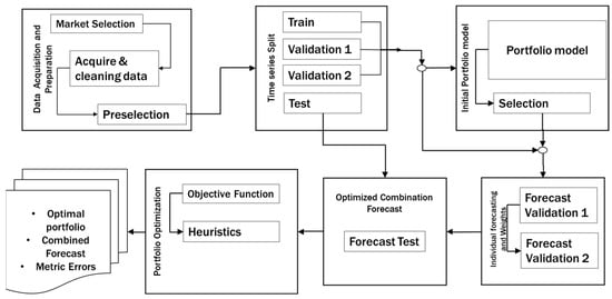
Figure 1.
The MASIP methodology.
3.1. Data Acquisition and Preparation
Market selection is the first step to integrate the investment portfolio. At this point, the target market to be analyzed is selected; among the candidate markets to be evaluated, we could mention those listed in the New York Stock Exchange, the European region, the Asian region, or those belonging to developing countries such as BRICS or Latin America. In this case, the analyst must perform a previous analysis of the target market and establish the period to be analyzed. In acquisition and cleaning of data, the information on each of the candidate assets is obtained. We consider the daily closing prices to conform to the time series in a determined time. As we know, it is important to have quality, cleanliness, and order of information since, if erroneous or missing information is entered, we will have inaccurate conclusions that can lead to severe losses of resources. Likewise, the data must be complete; thus, the necessary techniques must be applied to enable the data series cleaning process. Some of the methods used may be normalization, other data transformation, inter- or extrapolation, application of simple averages, moving averages, or any other variation that allows us to have complete information without altering the quality of the data [46,47,48].
The selection of assets should be made before integrating the portfolio. At this point, the analyst knows which assets of the selected marketplace are already the candidates for integrating the optimal portfolio. Thus, only the corresponding time series would be used to design it, and the effort for this task can be reduced. For example, if we analyze SP500, one of the largest financial exchanges in the world, we will have to analyze more than 500 time series, which consumes a lot of time and resources. To streamline the evaluation process, we apply the discrimination of assets that meet a percentage of profit or return by the Minimum Acceptable Rate of Return or MARR [49], which could be used to select an investment that assures us a fixed return with minimal utility and no risk. Thanks to this scheme, we can significantly reduce the number of candidate assets that need to be evaluated [8].
3.2. Time Series Split
The segmentation of time series is an important practice since it allows for evaluating the performance of models using known data and comparisons with previously unseen data. When a model is trained with a time series, it is expected to be able to make accurate predictions. However, if the model is evaluated with the same training data, there is a risk of overfitting, and only training data are stored.
When the time series data are divided into training, validation, and test sets, it is possible to adjust the model parameters to minimize the error in the validation set and then evaluate the model performance in the test set, which contains data that are “new” to the model and not previously analyzed.
Segmentation also allows for the identification of problems with the data, such as outliers or anomalous values, which allows for treating and correcting the input data before training the models and obtaining a final model [35,50,51].
In this implementation, the training portion of each time series is initially employed to forecast the validation section, applying all available individual forecast methods. The outcomes of this process are used to determine the most effective methods for forecasting the validation section and to establish the distribution of weights for the combination of these optimal methods. Subsequently, the forecast is evaluated using the validation data, and the most effective methods are identified, along with the previously calculated weight distribution. The resultant forecasts are stored, and the optimization process with TA is initiated using Validation 1 to forecast Validation 2. The weights are adjusted until no further improvement is observed [30].
3.3. Initial Portfolio Model
Building a portfolio is not a simple task today since several factors can influence the selection, integration, and weighting of the assets of the investment portfolio. That is why it requires robust and reliable tools which allow us to analyze many candidate assets and the data that integrate them. As we present in Section 1, the MPT model (Equations (1)–(4)), proposed by Markowitz, is the pioneering work in portfolio management which considers two main objectives: maximizing the expected return and minimizing the risk [3,52]. The Sharpe model represented by Equations (5)–(7) is an MPT extension considering the two objective functions in only one. In the present work, we propose a like-Markowitz Model of MASIP defined by Equations (8)–(12).
subject to
where is the expected return, i and j are the assets, is the portfolio risk, are the contribution of i and j assets, are the standard deviation of the assets, are the correlations between assets i and j, and is the Maximum Risk Rate Allowable.
The MASIP model defined by Equations (8)–(12), as we mentioned above, is an MPT extension with the following differences:
- In the objective function, we used the parameter MARR to represent the Minimum Acceptable Rate of Return that the investor could accept; instead, the Markowitz model uses a risk-free rate;
- Constraint (10) uses the MARR parameter for weighting assets into the portfolio;
- Constraint (12) uses the risk parameter to define the assets integrating the portfolio. This parameter binds the risk associated with the asset.
We use the parameter MARR, representing a common aspect used by decision-makers to accept an investment; however, the MPT and other models use a risk-free rate. Moreover, the average is sensitive to outliers and can be affected by extreme fluctuations. Conversely, the Expected Value (mathematical expectation) is calculated by multiplying each possible value by its probability of occurrence and adding up the results. In short, while the average is a basic measure of central tendency, the expected value more accurately represents the inherent uncertainty in the data [53].
In the state-of-the-art methods, a genetic algorithm is used for initial portfolio selection (GENPO), as well as algorithms based on threshold acceptance (TAIPO) and simulated annealing (SAIPO), which were tested and showed superior performance to other models, mainly focused on risk management (Yu, Gilli, and Masese) [16,17,54]. The last models are cited in the present study as YGM models. The individual YGM models versus MASIP are analyzed. The results of this analysis demonstrate the performance of the 12 combinations obtained between the YGM models and the hybridized algorithms. These results show that the YGM models using the maximum SR objective function applying the TAIPO algorithm obtain superior performance [8].
3.4. Individual Forecasting and Weights
Forecasting the performance of an investment portfolio is crucial for various reasons, such as identifying and quantifying the risks associated with the portfolio, financial planning, and evaluating strategy. Forecasting enables financial analysts to anticipate and adjust to changing market conditions, allowing them to make more timely and effective decisions.
The forecasting section of the Methodology is supported by FCTA (Forecasting Combined Method with Threshold Accepting) [30], which consists of assembling 14 forecasting methods and an enhanced threshold-accepting algorithm for weighting individual predictions. The forecast methods involved are Autoregressive integrated moving average ARIMA, exponential smoothing state space (ETS), Neural network forecasting method NNetar, Exponential smoothing state space-Box-Cox-ARMA (ETS), STLM with AR method, Naive and random walk forecasts with drift activated, Decomposing Time Series with Smoothing Methods (Theta), Naïve method, Autoregressive fractionally integrated moving average (ARFIMA), Bootstrapped method (Bagged), SplinesCubic, Holt, Feature-based forecast model averaging (FFORMA), and Jaganathan.
Notably, at least two of the models incorporated, FFORMA [36] and Jaganathan [55], obtained second and fourth place, respectively, in the competition, as both FFORMA and Jaganathan are ensemble and hybridization methods in certain cases [56]. Within this framework, it is essential to underscore the more than 24,500 financial series within the dataset, which suggests that the application of FCTA for the analysis of financial series can be considered reliable.
The FCTA employs a set of criteria to evaluate the efficacy of forecasting methods, including the uniform distribution, the normalized weights criterion, the Bayesian information criterion (BIC), and the Akaike information criterion (AIC). These criteria have been demonstrated to yield superior performance in the analysis and forecasting of the M4 competition series, which encompasses financial series.
The forecasting process is presented in Figure 2. In this stage, individual forecasts are made for each asset and its time series, using each forecasting technique considered in the algorithm, that is, the n assets selected in the initial portfolio are evaluated and forecasted by the M forecasting models. This is performed for each split of the time series, that is, each of the forecasting models is fed with the training section of each of the asset’s data and compared with the validation section. The error is measured for all the best methods, and the ones with the lowest error evaluation are selected and compared against the test section.
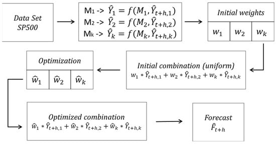
Figure 2.
Combination of forecasting methods.
The initial combination of forecasting methods is established through the selection of the best-evaluated ones.
Through experiments involving enhanced weights, it was observed that a collection of methods yielded superior results compared to individual methods. They identified which features were crucial for selecting methods for the combination. Notice that the most effective combination is typically achieved when the best individual methods are employed.
Since the mid-20th century, ensemble methods for forecasting have been applied [57]; specifically, Bates [9] proposed using several forecasting methods in a weighted combination with weights w to be determined in terms of the error of each of the individual methods. This method is commonly known as the Bates method and was initially tested using Brown’s exponential smoothing methods. The way to compare n ≥ 2 methods in the Bates method is to determine the Mean Squared Error (MSE) for all methods for the series considered in an evaluation period; then, the methods are combined so that each participates in the forecast in terms of the accuracy corresponding to its MSE. A final forecast ensemble or combination can be expressed as Equation (13):
It can be said that the relationship between the combined forecast and the individual forecast are linear, where we have individual forecast models, and for each model we have a weight .
Moreover, the objective function is measured using the symmetric mean absolute percentage error (sMAPE), a variation of the classic mean absolute percentage error (MAPE) metric [58]. However, other convenient error metrics could be used. The metric used in this paper is expressed in Equation (14).
where is the current observation of the time series, represents the predicted value, is the amount of data in the time series, and represents the length of the forecast horizon. This measure has been the subject of analysis since the late 1980s [59], but it gained popularity with the M3 competitions [60,61] as a metric to compare various forecasting methods. sMAPE is simple to calculate and understand, and unlike other errors, sMAPE considers both overestimates and underestimates equally.
Other error metrics considered for evaluation are MSE (15), Root Mean Squared Error (RMSE) (16), and Mean Absolute Percentage Error (MAPE) in Equation (17).
In the context of machine learning forecasting, the evaluation of model performance is subject to selecting appropriate metrics. This study includes MSE, MAPE, and RMSE to evaluate forecasting models. MSE is used as an objective function because of its ability to penalize large errors, although its sensitivity to outliers can be a disadvantage. MAPE can overestimate small errors and generate problems when actual values are close to zero. sMAPE, on the other hand, is used to present results which are easy to understand, as it provides a more symmetric error penalty compared to MAPE [62]. While MSE is useful for optimizing models, its interpretation is not intuitive for users. Therefore, sMAPE is used for internal model fitting, while MSE is used for algorithm comparison. This approach is designed to ensure a comprehensive and equitable evaluation of forecasting models, aligning with practices employed in time series forecast competitions [63].
The RMSE is useful in cases where large errors are unacceptable because it takes the square root of the errors. This makes the RMSE the same size as the original variable, which makes it easier to understand the average size of the error. However, it can also be too harsh on big errors, which may be a problem if they are rare or not important in the analysis. Outliers can also have a big effect on the RMSE, which can change how we judge the model when there are outliers [35]. The coefficient of the determination Rsquared (R2) measures how well a forecasting model explains the variability of the actual data [35].
3.5. Optimized Combination Forecast
Once an initial combination of forecasting methods is obtained using the best-evaluated models, it is necessary to establish the optimal combination of the forecast models, i.e., to weigh them in such a way that this combination delivers the lowest possible error. For this, it is necessary to use again the heuristics that allow solutions, which, in this case, try to minimize the error of the combined forecast against real test data. As mentioned above, it is possible to use any of the heuristic methods.
Figure 3 shows the general process of the FCTA methodology. In the first step, the training data of the n time series are used in the m forecasting methods, . These methods generate a weighted combination of methods for each time-series. This combination is then compared to validation segment 1. The process is repeated with the data of Validation 1. These data are used to forecast into the periods of Validation 2. The results are then compared to Validation 2. The test split is applied to evaluate the optimized combined forecasting. The error analysis in stages 1 and 2 selects the best individual forecasting methods for each of the selected assets in the initial portfolio, thereby establishing an initial mix of forecasting methods. This combination is uniform when equal weights are assigned to each forecasting method.
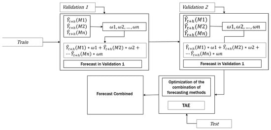
Figure 3.
General outline of FCTA.
The initial combination of the best forecasting methods enters the optimization heuristic based on TA, which has been modified to obtain a superior performance to the classical TA algorithm. The algorithm Threshold Accepting Enhanced (TAE) is an algorithm including a modified cooling scheme, a reheating scheme, and thermal equilibrium. This algorithm was tested and showed a high performance in M4 time series [30].
The output of the TAE algorithm is the weighted combination of the best forecasting methods that obtain the minimum value of the sMAPE error metric. The weighted methods are then combined to generate forecasts, which are subsequently compared against the test section to calculate the error metric.
3.6. Portfolio Optimization
Following the conclusion of the forecasting process, it is imperative to perform a portfolio rebalancing or optimization. In this stage, the candidate assets’ past and forecasted data are evaluated using the methodologies or algorithms outlined in Section 3.3. The anticipated outcome of this process is a portfolio that exhibits enhanced performance in comparison to its initial state. The logical sequence and steps of MASIP are shown in Algorithm 1.
| Algorithm 1. Pseudo code for MASIP methodology | |
| 1: | Market: Time series for portfolio forecasting (assets) Result: Optimal Portfolio Forecast |
| 2: | Initialization |
| 3: | Market <- Get Market data Market <- Clear Market data |
| 4: | For i in each asset in the Market |
| 5: | If profit_asset >= MARR #Minimum Acceptable Rate Return |
| 6: | Data <- asset |
| 7: | Train, validation 1, validation 2, Test <- splitData() |
| 8: | InitialPortfolio <- PortfolioSelection(Data[Train, validation 1, validation 2], ObjectiveFunction) |
| 9: | IndividualForecast <- IndividualMethods(Data[InitialPortfolio]) |
| 10: | InitialCombinationMethod <- IncludeProcess(IndividualForecast) |
| 11: | ForecastCombination <- FCTA(InitialCombinationMethod, Test) |
| 12: | OptimalPortfolio <- PortfolioSelection(Data[Train, validation 1, validation 2, Test], ForecastCombination) |
| 13: | Return (Optimal portfolio, Combined Forecast, Metric Errors) |
4. Experimentation and Results
This section reviews the equipment and material resources used for developing this study. Since this is complex work, several computer parts equipment were required: Intel(R) Core(TM) i7-13620H, CPU @ 2.40 GHz, RAM: 16 GB, Intel(R) Xeon(R) Gold 6230 CPU @ 2.10 GHz, and 2.10 GHz, RAM: 12 GB (National Laboratory of Information Technology, Tamaulipas, Mexico).
The languages used for this experiment are Python 3.7 for initial and final portfolios and R 4.3.3 for forecasting.
A description of the time series utilized and an account of the experimentation conducted with this series through the portfolio integration and portfolio forecasting algorithms are also provided. A concise overview of both is included. The results and discussion of these experiments are subsequently presented.
4.1. Methodology Application
In this section the methodology application is described in detail and each step of our methodology is explained from the data acquisition and preparation to the final portfolio optimization.
4.1.1. Data Set Acquisition and Preparation
To evaluate the algorithms and the proposed solution methodology, a set of assets and their data series of the SP500 were used, consisting of 479 companies listed between January 2020 and the end of February 2025, giving a total of 262 observations (weekly prices). This period was chosen because there was significant variability in the index and the stocks due to the health emergency that affected the assets of the United States of America and the whole financial world.
Justifications for using the SP500 are the market representativeness and diversification (wide variety of companies of different sectors and sizes), access to historical data, liquidity which allows for easy and efficient trading, it being commonly used as a benchmark to compare the performance of an investment portfolio, and, finally, the U.S. equity market enjoys strong regulation and institutional stability.
A computer program was developed to obtain information on the SP500 market assets corresponding to the daily closing prices of the selected period from the Yahoo Finance portal. Once the initial set was formed, the amount of empty or non-numeric data (NAN) was checked, and those with missing data representing more than 50% of the total were discarded.
In the first phase of the proposed model, data validation and cleaning were performed, which consisted of verifying that all the assets had the complete and correct information for the period to be analyzed. The main tasks performed in this phase were detecting atypical data and data supplementation in case of missing data at the beginning, end, or within the series. The complementation process was performed by applying the extrapolation (missing data at the beginning or end of the series) and interpolation methods.
As a final step, the expected value of each asset was compared to the return of the SP500 index, as shown in Figure 4, where the assets with a return lower than this value were discarded, since the assets that do not exhibit a return higher than this limit would be of no interest to financial investors. As mentioned above, this helps to reduce computation time since the final set of data to be analyzed is reduced.
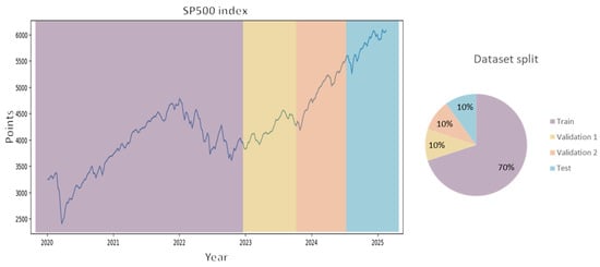
Figure 4.
SP500 performance and split.
4.1.2. Segmentation of the Data Set
At this point, it was decided to segment the data series into four sections: the first segment is the training set, which was established as 70% of the data, i.e., 183 weekly observations, two validation segments, which consist of 10% of the observations each, i.e., 26 observations each, and finally a test segment equivalent to the remaining 10%. We decided to segment in this way to make the dataset compatible with the techniques applied in the FCTA methodology for data forecasting. Similarly, this same segmentation is applicable in constructing the initial portfolio where the training and validation sets are taken as input data. To summarize, the segmentation written above is in Figure 4.
4.1.3. Initial Portfolio Hyperparameters
For the construction of the initial portfolio, the TAIPO algorithm was used. This had already been tested and compared previously with other alternatives, demonstrating its advantages, such as obtaining high values in the Sharpe Ratio as well as a good return and a low correlation of assets.
The hyperparameters of the TAIPO metaheuristic were tuned by applying the analytical tuning method described in [8,64]. The values obtained for the parameters are: Initial Temperature: 273.8164, Final Temperature: 0.0000169, Cooling ratio: 0.96, while the equilibrium cycle length L, was dynamically calculated as a function of the number of assets and the temperature scheme.
Given that TAIPO is an approximate algorithm, 30 executions were carried out to obtain the average of the performance indicators, thereby enabling the selection of assets that maximize returns. The average values obtained were: Sharp Ratio (SR): 0.0221, Return: 0.0114, Risk: 0.2980, Correlation between assets: 0.2044, and the number of selected assets: 57, in weekly terms.
Compared to the performance of the SP500 during 2024, equivalent to 0.24 per year, the portfolio integrated in this stage had a performance of 147% above the index.
Figure 5 shows a sample of the graphs generated by the results of the algorithm. It can be observed that the Sharpe Ratio behaves as expected regarding the TAIPO algorithm; in the initial interactions, the system tolerates suboptimal solutions. However, as the iterations progress under the cooling scheme, the system becomes less tolerant of accepting bad solutions, ultimately identifying a higher SR value.
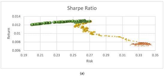
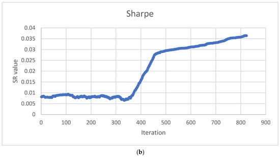
Figure 5.
Algorithm performance in optimizing the Sharpe-based objective function value. (a) Efficient Frontier Risk vs. Return; (b) Sharpe Ratio values through algorithm execution.
Figure 5a presents the growth of the Sharpe Ratio value, which provides a representative example of the algorithm’s performance. The size of the bubbles represents the SR, with smaller bubbles in the lower part corresponding to SR values between 0.0 and 0.01, indicating lower returns (below 0.008). In the intermediate section, the SR values range from 0.01 to 0.0299, with returns varying between 0.008 and 0.012. The larger bubbles at the top illustrate the efficient frontier, which is defined as a set of portfolios with high SR values above 0.03 and returns greater than 0.012.
The behavior of the SR value, which functions as the evaluation criterion for the TAIPO algorithm, is highlighted and shown in Figure 5b. Up to iteration 350, the values exhibit the anticipated behavior, accepting suboptimal solutions. However, after this initial phase, there is a decline in the acceptance of suboptimal solutions, leading to enhanced SR values. Notice that from iteration 500 to the conclusion of the process, the highest SR values correspond to the efficient frontier.
4.1.4. Forecasting: Weights and Optimization
For the initial portfolio forecasting, we applied the FCTA predicting tools [30]. Figure 6 shows the average result of the fourteen forecasting methods; we executed thirty executions according to the FCTA process. The sMAPE metric is presented for the initial combination using a uniform (sMAPE U) distribution for the weights. A 35.28% value was obtained for this initial solution, while the optimized combination (sMAPE O) yielded a sMAPE value of 23.60%. Notice that a large improvement of 49% of sMAPE was obtained. The forecast horizon for this case was set at 7 weeks ahead; nevertheless, MASIP works for any other short and medium forecast horizon.
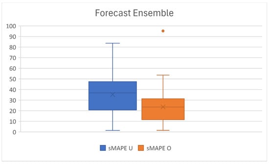
Figure 6.
Forecast ensemble metric.
As illustrated in Table 2, a comparison is presented that integrates four performance error metrics.
Table 2.
Forecasting performance of FCTA from 2020 to 2025.
4.1.5. Final Portfolio Optimization
In the final stage of the methodology, the combined forecasts of the assets were obtained. These were then refined using one of the integration algorithms and objective functions that have been previously mentioned. For this phase, the TAIPO algorithm was employed once more with the following metrics: Sharp Ratio: 0.0359, Return: 0.0126, Risk: 0.2170, Correlation between assets: −0.1061, and number of selected assets: 6 incorporating the complete time series as well as the forecasts calculated in the preceding stage. In terms of performance, the final portfolio presented an increase of 10.5% in returns and a reduction in correlation value compared to the initial portfolio. The graph of the evolution of the Sharpe-based objective function is shown in Figure 7.
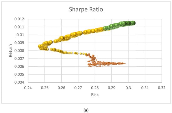
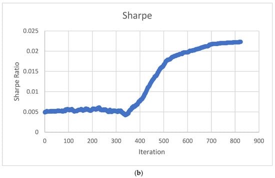
Figure 7.
The Sharpe Ratio during final portfolio optimization: (a) Sample of Sharpe Ratio portfolios; (b) Sharpe Ratio through the TAIPO algorithm.
Figure 7a presents the growth of the Sharpe Ratio value, which provides a representative example of the algorithm’s performance. The size of the bubbles represents the Sharpe Ratio (SR), with smaller bubbles in the lower part corresponding to SR values between 0.0 and 0.0099, indicating lower returns (below 0.00756). In the intermediate section, the SR values range from 0.01 to 0.02, with returns varying between 0.0075 and 0.0108. The larger bubbles represent the efficient frontier, which is defined as a set of portfolios with high SR values above 0.022 and returns greater than 0.011. The behavior of the SR value is presented in Figure 7b, which serves as the evaluation function for the TAIPO algorithm; up to iteration 250, the values behave as expected, accepting suboptimal solutions. However, in some periods ahead, the acceptance of suboptimal solutions decreases, resulting in better SR values. From iteration 310 to completion, the highest SR values form the efficient frontier. We can, therefore, conclude that the algorithm finds the best solutions and begins a stagnation process. This means that after 20 repetitions of the algorithm without finding an improvement in the solution, the algorithm stops [8].
By way of comparison and observing the results of the performance of the GENPO algorithm, an experiment was carried out for the optimization of the final portfolio, producing the following results: SR: 0.0308, Return: 0.0132, Risk: 0.2399, Correlation between assets: −0.0674, and number of selected assets: 10. In the results, we notice that, in practically all the items, there are similar values except for the assets where there are 10, as well as a slight increase in both return value and risk.
4.2. MASIP Comparison with State-of-the-Art Methods
To validate the proposed methodology, we compared MASIP with Puerto and Cesarone’s model [21,23], and we used datasets from the SP500 market from 2005 to 2016. This period comprises the widest range of time common in both studies. For these datasets, we compared the average MASIP results with those reported by these authors in Table 3. In the last references, a portfolio for 52 weeks considering a zero risk-free rate was performed. The metrics used in the three alternatives were: the expected return, the risk value, the Sharpe Ratio, and the number of assets. These results are discussed in subsequent sections. We developed the programming codes necessary to emulate the former authors’ works.
Table 3.
MASIP results comparison with state-of-the-art methods for SP500.
4.2.1. Data Acquisition, Preparation, and Split
We gathered datasets between 2005 and 2016 using Yahoo Finance, comprising, after data cleaning, a preparation dataset of 445 assets and 572 weekly observations. Observations were split into 70% for training, 10% each for Validation 1 and 2, and 10% for testing.
4.2.2. Initial Portfolio MARR Results
The TAIPO algorithm was used to build the initial portfolio, with the maxSharpe model. Table 4 shows a sensitivity analysis of the average results of the portfolios with different minimum acceptable rates of return (MARR). The value of the SR is directly related to the value of the MARR, since as the return value increases, the algorithm will look for a set of assets that delivers a higher return. We can also observe that as the minimum acceptable rate of return increases, the number of assets decreases; this is because, internally, the algorithm selects the assets with the highest return and that is close to the risk-free value. On the other hand, the results show a slight reduction in the correlation value.
Table 4.
Initial portfolio applying MARR.
The improvement in SR values achieved by the TAIPO algorithm and the target function can be seen in Figure 8.
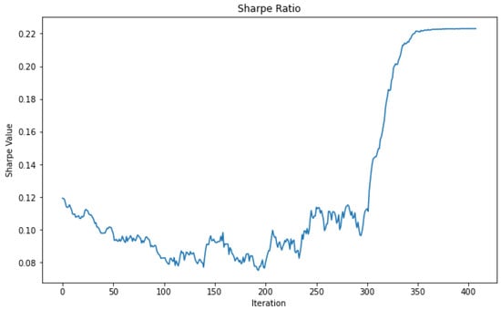
Figure 8.
Sample of Sharpe Ratio in the initial portfolio.
4.2.3. Portfolio Forecasting
The initial portfolio was generated with the heuristic algorithm, and individual forecasts were obtained for each selected asset through the 14 forecasting methods within the FCTA methodology. A series of experiments were conducted, varying the forecast horizon within the range of 1 to 24 weeks.
Table 5 shows the differences in the error metric values of the forecast method combination models in a uniform distribution scheme, sMAPE U, and the contrast with the sMAPE O.
Table 5.
Average sMAPE values at different forecasting horizons.
In conclusion, the application of the FCTA algorithm, once more, provides results that, at least in the case of the 1-week forecast horizon, demonstrate an improvement of up to 50%.
As is shown in Table 6, a comparison is presented that integrates four performance error metrics.
Table 6.
Forecasting performance of FCTA from 2005 to 2016.
4.2.4. Final Optimized Portfolio
The subsequent section entails implementing rebalancing or optimization procedures. For this purpose, the TAIPO algorithm was used to obtain comparative results for each forecast horizon, as well as to contrast the advantages of each of the algorithms and the case study. It becomes evident that as the forecast horizon increases, there is a notable decline in the Sharpe Ratio and return values. Concurrently, the risk factor experiences a reduction, and the number of assets exhibits a decline. The performance shown in Figure 9 illustrates the evolution of the SR within the algorithm for the integration of the final portfolio. The final portfolios generated through MASIP methodology exhibit Sharpe values that are higher than those of the state-of-the-art methods in the short term, and this advantage is further enhanced once these portfolios have been forecasted. As we observe, they maintain or even increase the SR in the presented instances.
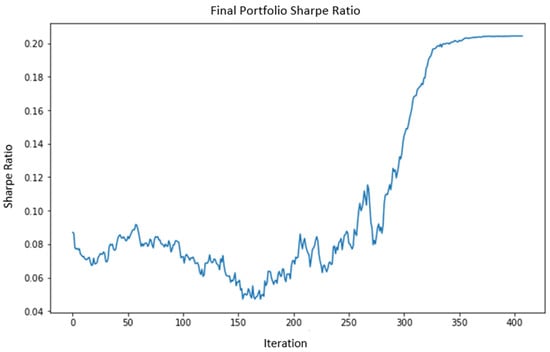
Figure 9.
Sample of Sharpe Ratio in the final portfolio.
Table 7 shows the results obtained from these experiments, prioritizing the average of the highest Sharpe values found, identifying the algorithms that achieved superior performance in return terms. As shown in Table 7, the integrated portfolios with brief time horizons and the model MASIP yield outcomes surpass the contemporary standard. Conversely, in the medium-term horizons, between 8 and 24 weeks, Cesarone’s model attains superior results in terms of SR. Conversely, when the focus is directed toward the variable yield, the MASIP algorithm demonstrates a markedly superior performance in comparison to the other two algorithms. This distinction can be attributed to the inherent characteristics of the MASIP algorithm and the mathematical models employed. The MASIP model is designed to optimize the SR by prioritizing the maximization of yield.
Table 7.
Final comparison of forecasted values.
Conversely, the implementation of the MASIP methodology in the models under comparison yields analogous or superior outcomes. This is evident in the case of the Puerto approach, where predictions for the medium term (i.e., 8 to 24 weeks) indicate an SR considerably higher than those reported in the reference studied, reaching up to 415%. In contrast, Cesarone’s model consistently shows superior performance, particularly in medium-term predictions, where significant improvements of up to 348% in terms of the SR are observed. As mentioned above, the MASIP methodology can be applied with various models, yielding favorable outcomes.
5. Conclusions
This paper proposes MASIP, an efficient methodology for investing portfolios. This methodology presents for the first time all the elements required for designing a portfolio: the selection of the best asset candidates for integrating the portfolio, the forecasting of the asset values in the investing horizon, including the best method selection for this task, the integration the best assets in this horizon and their participation, as well as the optimization model considering new constraints related to the maximum risk rate allowable and the minimum acceptable rates of return. MASIP was applied to SP500 and compared with state-of-the-art methods.
Regarding the initial phase of the portfolio construction process, it is imperative to identify the most suitable candidates. To this end, MASIP employs the TAIPO algorithm, a proposed mathematical model, and a constraint related to the lowest acceptable rate of return. This approach facilitates the identification of effective portfolios. In a subsequent stage, MASIP employs the FCTA to generate individual forecasts for each candidate asset and each of the prediction methods, selecting those methods with optimal performance and assembling them through the TAE algorithm to identify the optimal combination that minimizes the sMAPE and generates short- and medium-term forecast horizons. A rebalancing of the portfolio is subsequently implemented in the final stage, utilizing the TAIPO algorithm. This results in a portfolio comprising forecasted data and optimized weightings.
Experimental evaluations of the algorithms and data used yielded outstanding asset selection and evaluation results with SR, as well as expected return. The MASIP methodology was complemented by the forecast of the assets participating in the portfolio, thus collaborating in the final optimization, resulting in a final weighted, forecasted, and optimized portfolio.
A comparative analysis was conducted between MASIP and two alternative investment models, the Puerto and Cesarone models. The outcomes of this analysis were prioritized based on the meaning of the highest Sharpe values identified. The results of this study demonstrate that the MASIP algorithm exhibited robust performance in terms of returns. As the forecast horizon grows, the SR and return values drop significantly, concurrently with a drop in the risk factor and the asset number. The SR values from the created portfolios exceed those of the state-of-the-art methods, and forecasting enhances this advantage. The superiority of MASIP performance relative to the other two algorithms lies in its design, which prioritizes the maximization of short-term yield to optimize SR. Furthermore, the efficacy of the MASIP methodology in enhancing the performance of other methodologies is evident from the observed improvement in SR performance. This observation supports the potential for further experimentation with the same approach.
For future research, the application of other optimization methods is proposed, including other objective functions and metrics, both for asset preselection and portfolio rebalancing, the experimentation of novel methods or forecasting ensembles in financial time series, as well as the application of the MASIP methodology in other markets.
Author Contributions
Conceptualization, J.F.-S. and J.P.-A.; methodology and software, J.P.-A.; validation, G.C.-V., J.G.-B. and J.F.-S.; formal analysis, J.F.-S. and J.G.-B.; investigation, J.P.-A. and J.F.-S.; writing—original draft preparation, J.P.-A.; writing—review and editing, J.G.-B., J.F.-S., J.P.S.H. and G.C.-V.; supervision, J.F.-S. and J.G.-B.; project administration, J.F.-S. All authors have read and agreed to the published version of the manuscript.
Funding
This research received no external funding.
Data Availability Statement
https://github.com/DrJuanFraustoSolis/TAIPO.git (accessed on 30 January 2025).
Acknowledgments
The authors would like to acknowledge SECIHTI (Secretariat of Science, Humanities, Technology and Innovation), TecNM (National Technology of Mexico), Madero City Technological Institute, and the National Laboratory of Information Technologies (LaNTI) for access to the cluster.
Conflicts of Interest
The authors declare no conflicts of interest.
References
- Guerard, J.B. Introduction to Financial Forecasting in Investment Analysis, 1st ed.; Springer: New York, NY, USA, 2013. [Google Scholar] [CrossRef]
- Andersen, J.V. Investment Decision Making in Finance, Models of. In Encyclopedia of Complexity and Systems Science; Meyers, R.A., Ed.; Springer: New York, NY, USA, 2009; pp. 4971–4983. [Google Scholar] [CrossRef]
- Markowitz, H. Portfolio Selection. J. Financ. 1952, 7, 77–91. [Google Scholar] [CrossRef]
- Sharpe, W.F. Mutual Fund Performance. J. Bus. 1966, 39, 119–138. [Google Scholar] [CrossRef]
- Scholz, H. Refinements to the Sharpe ratio: Comparing alternatives for bear markets. J. Asset Manag. 2007, 7, 347–357. [Google Scholar] [CrossRef]
- Zakamouline, V.; Koekebakker, S. Portfolio performance evaluation with generalized Sharpe ratios: Beyond the mean and variance. J. Bank. Financ. 2009, 33, 1242–1254. [Google Scholar] [CrossRef]
- Landete, M.; Monge, J.F.; Ruiz, J.L.; Segura, J.V. Sharpe Portfolio Using a Cross-Efficiency Evaluation BT—Data Science and Productivity Analytics; Charles, V., Aparicio, J., Zhu, J., Eds.; Springer International Publishing: Cham, Switzerland, 2020; pp. 415–439. [Google Scholar] [CrossRef]
- Solis, J.F.; Aldaz, J.L.P.; Del Angel, M.G.; Barbosa, J.G.; Valdez, G.C. SAIPO-TAIPO and Genetic Algorithms for Investment Portfolios. Axioms 2022, 11, 42. [Google Scholar] [CrossRef]
- Bates, J.M.; Granger, A.W.J. The Combination of Forecasts. Oper. Res. Soc. 1969, 20, 451–468. [Google Scholar] [CrossRef]
- Winkler, R.L.; Makridakis, S. The Combination of Forecasts. J. R. Stat. Soc. Ser. A 1983, 146, 150–157. [Google Scholar]
- Dueck, G.; Scheuer, T. Threshold accepting: A general purpose optimization algorithm appearing superior to simulated annealing. J. Comput. Phys. 1990, 90, 161–175. [Google Scholar] [CrossRef]
- Winker, P.; Maringer, D. The Threshold Accepting Optimisation Algorithm in Economics and Statistics. In Optimisation, Econometric and Financial Analysis; Kontoghiorghes, E.J., Gatu, C., Eds.; Springer: Berlin/Heidelberg, Germany, 2007; pp. 107–125. [Google Scholar]
- Choueifaty, Y.; Coignard, Y. Toward maximum diversification. J. Portf. Manag. 2008, 35, 40–51. [Google Scholar] [CrossRef]
- Tella, R.; Rogel-Salazar, J. Portfolio Construction Based on Implied Correlation Information and VAR. SSRN Electron. J. 2013, 12, 125–144. [Google Scholar] [CrossRef]
- Wang, S.; Xia, Y. Portfolio Selection and Asset Pricing, 1st ed.; Springer: Berlin/Heidelberg, Germany, 2002. [Google Scholar] [CrossRef]
- Gilli, M.; Këlezi, E. A Heuristic Approach to Portfolio Optimization. Available online: https://citeseerx.ist.psu.edu/document?repid=rep1&type=pdf&doi=f6500f280e2c91a2ce11d0e46f90424aaac749f4 (accessed on 31 January 2025).
- Masese, J.M.; Othieno, F.; Njenga, C. Portfolio Optimization under Threshold Accepting: Further Evidence from a Frontier Market. J. Math. Financ. 2017, 7, 941–957. [Google Scholar] [CrossRef][Green Version]
- Rangel-González, J.A.; Frausto-Solis, J.; González-Barbosa, J.J.; Pazos-Rangel, R.A.; Fraire-Huacuja, H.J. Comparative study of ARIMA methods for forecasting time series of the mexican stock exchange. Stud. Comput. Intell. 2018, 749, 475–485. [Google Scholar] [CrossRef]
- Vijh, M.; Chandola, D.; Tikkiwal, V.A.; Kumar, A. Stock Closing Price Prediction using Machine Learning Techniques. Procedia Comput. Sci. 2020, 167, 599–606. [Google Scholar] [CrossRef]
- Singh, P.; Jha, M. Portfolio Optimization Using Novel EW-MV Method in Conjunction with Asset Preselection. Comput. Econ. 2024, 64, 3683–3712. [Google Scholar] [CrossRef]
- Cesarone, F.; Scozzari, A.; Tardella, F. An optimization–diversification approach to portfolio selection. J. Glob. Optim. 2020, 76, 245–265. [Google Scholar] [CrossRef]
- Cesarone, F.; Mottura, C.; Ricci, J.M.; Tardella, F. On the Stability of Portfolio Selection Models. 2018, pp. 1–27. Available online: https://papers.ssrn.com/sol3/papers.cfm?abstract_id=3420081 (accessed on 31 January 2025).
- Puerto, J.; Rodríguez-Madrena, M.; Scozzari, A. Clustering and portfolio selection problems: A unified framework. Comput. Oper. Res. 2020, 117, 104891. [Google Scholar] [CrossRef]
- Kaczmarek, T.; Perez, K. Building portfolios based on machine learning predictions. Econ. Res. Istraz. 2021, 35, 1–19. [Google Scholar] [CrossRef]
- Zhang, A. Portfolio Optimization of Stocks—Python-Based Stock Analysis. Int. J. Educ. Humanit. 2023, 9, 32–38. [Google Scholar] [CrossRef]
- Ma, Y.; Han, R.; Wang, W. Portfolio optimization with return prediction using deep learning and machine learning. Expert Syst. Appl. 2021, 165, 113973. [Google Scholar] [CrossRef]
- Martínez-Barbero, X.; Cervelló-Royo, R.; Ribal, J. Portfolio Optimization with Prediction-Based Return Using Long Short-Term Memory Neural Networks: Testing on Upward and Downward European Markets. Comput. Econ. 2024, 65, 1479–1504. [Google Scholar] [CrossRef]
- Elliott, G.; Timmermann, A. Economic Forecasting. J. Econ. Lit. 2008, 46, 3–56. [Google Scholar] [CrossRef]
- Centeno, V.; Georgiev, I.R.; Mihova, V.; Pavlov, V. Price forecasting and risk portfolio optimization. AIP Conf. Proc. 2019, 2164, 060006. [Google Scholar] [CrossRef]
- Frausto-Solis, J.; Rodriguez-Moya, L.; González-Barbosa, J.; Castilla-Valdez, G.; Ponce-Flores, M. FCTA: A Forecasting Combined Methodology with a Threshold Accepting Approach. Math. Probl. Eng. 2022, 2022, 6206037. [Google Scholar] [CrossRef]
- Zhang, Y.; Qu, H.; Wang, W.; Zhao, J. A Novel Fuzzy Time Series Forecasting Model Based on Multiple Linear Regression and Time Series Clustering. Math. Probl. Eng. 2020, 2020, 9546792. [Google Scholar] [CrossRef]
- Rao, P.S.; Srinivas, K.; Mohan, A.K. A Survey on Stock Market Prediction Using Machine Learning Techniques BT—ICDSMLA 2019; Kumar, A., Paprzycki, M., Gunjan, V.K., Eds.; Springer: Singapore, 2020; pp. 923–931. [Google Scholar]
- Becha, M.; Dridi, O.; Riabi, O.; Benmessaoud, Y. Use of Machine Learning Techniques in Financial Forecasting. In Proceedings of the 2020 International Multi-Conference on: “Organization of Knowledge and Advanced Technologies” (OCTA), Tunis, Tunisia, 6–8 February 2020; pp. 1–6. [Google Scholar] [CrossRef]
- He, K.; Yang, Q.; Ji, L.; Pan, J.; Zou, Y. Financial Time Series Forecasting with the Deep Learning Ensemble Model. Mathematics 2023, 11, 1054. [Google Scholar] [CrossRef]
- Hyndman, R.J.; Athanasopoulos, G. Forecasting: Principles and Practice. In Forecasting: Principles and Practice; Econometrics & Business Statistics: Monash, Australia, 2018; p. 504. Available online: https://otexts.com/fpp2/ (accessed on 31 January 2025).
- Montero-Manso, P.; Athanasopoulos, G.; Hyndman, R.J.; Talagala, T.S. FFORMA: Feature-based forecast model averaging. Int. J. Forecast. 2020, 36, 86–92. [Google Scholar] [CrossRef]
- Petropoulos, F.; Apiletti, D.; Assimakopoulos, V.; Babai, M.Z.; Barrow, D.K.; Ben Taieb, S.; Bergmeir, C.; Bessa, R.J.; Bijak, J.; Boylan, J.E.; et al. Forecasting: Theory and practice. Int. J. Forecast. 2022, 38, 705–871. [Google Scholar] [CrossRef]
- Estrada-Patiño, E.; Castilla-Valdez, G.; Frausto-Solis, J.; González-Barbosa, J.; Sánchez-Hernández, J.P. A Novel Approach for Temperature Forecasting in Climate Change Using Ensemble Decomposition of Time Series. Int. J. Comput. Intell. Syst. 2024, 17, 253. [Google Scholar] [CrossRef]
- Wasserbacher, H.; Spindler, M. Machine learning for financial forecasting, planning and analysis: Recent developments and pitfalls. Digit. Financ. 2022, 4, 63–88. [Google Scholar] [CrossRef]
- Dharrao, D.S.; Bongale, A.M.; Deokate, S.T.; Doreswamy, D.; Bhat, S.K. Forecasting Stock Market Prices Using Machine Learning and Deep Learning Models: A Systematic Review, Performance Analysis and Discussion of Implications. Int. J. Financial Stud. 2023, 11, 94. [Google Scholar] [CrossRef]
- Cheng, L.; Shadabfar, M.; Khoojine, A.S. A State-of-the-Art Review of Probabilistic Portfolio Management for Future Stock Markets. Mathematics 2023, 11, 1148. [Google Scholar] [CrossRef]
- Althöfer, I.; Koschnick, K.-U. On the convergence of ‘Threshold Accepting’. Appl. Math. Optim. 1991, 24, 183–195. [Google Scholar] [CrossRef]
- Winker, P. The Stochastics of Threshold Accepting: ANALYSIS of an Application to the Uniform Design Problem BT—Compstat 2006—Proceedings in Computational Statistics; Rizzi, A., Vichi, M., Eds.; Physica: Heidelberg, HD, USA, 2006; pp. 495–503. [Google Scholar]
- Gilli, M.; Kellezi, E. The Threshold Accepting Heuristic for Index Tracking. In Financial Engineering, E-commerce and Supply Chain; Springer: Boston, MA, USA, 2011; pp. 1–18. [Google Scholar] [CrossRef]
- Ta, V.D.; Liu, C.M.; Tadesse, D.A. Portfolio optimization-based stock prediction using long-short term memory network in quantitative trading. Appl. Sci. 2020, 10, 437. [Google Scholar] [CrossRef]
- Kelleher, J.D.; Tierney, B. Data Science; The MIT Press: Cambridge, MA, USA, 2018. [Google Scholar]
- Provost, F.; Fawcett, T. Data Science for Business: What You Need to Know About Data Mining and Data-Analytic Thinking, 1st ed.; O’Reilly Media: Sebastopol, CA, USA, 2013. [Google Scholar]
- Kuhn, M.; Johnson, K. Feature Engineering and Selection: A Practical Approach for Predictive Models, 1st ed.; CRC Chapman and Hall: Boca Raton, FL, USA, 2019. [Google Scholar]
- SRoss, A.; Westerfield, R.W.; Jordan, B.D. Fundamentals of Corporate Finance, 13th ed.; McGraw Hill: New York, NY, USA, 2021. [Google Scholar]
- Box, G.E.P.; Jenkins, G.M.; Reinsel, G.C. Time Series Analysis: Forecasting and Control; Prentice Hall: Englewood Cliffs, NJ, USA, 1994; Volume SFB 373, Chapter 5; pp. 837–900. [Google Scholar]
- Goodfellow, I.; Bengio, Y.; Courville, A. Deep Learning; MIT Press: Cambridge, MA, USA, 2016; Available online: http://www.deeplearningbook.org (accessed on 31 January 2025).
- Markowitz, H. Foundations of portfolio theory. In Harry Markowitz: Selected Works; World Scientific Publishing Company: Singapore, 2009; Volume 46, pp. 481–490. [Google Scholar] [CrossRef]
- Markowitz, H.M. Portfolio Selection; Yale University Press: New Haven, CT, USA, 1959; Available online: http://www.jstor.org/stable/j.ctt1bh4c8h (accessed on 31 January 2025).
- Yu, L.; Wang, S.; Lai, K.K. Multi-attribute portfolio selection with genetic optimization algorithms. INFOR 2009, 47, 23–30. [Google Scholar] [CrossRef]
- Jaganathan, S.; Prakash, P.K.S. A combination-based forecasting method for the M4-competition. Int. J. Forecast. 2020, 36, 98–104. [Google Scholar] [CrossRef]
- Cawood, P.; Van Zyl, T. Evaluating State-of-the-Art, Forecasting Ensembles and Meta-Learning Strategies for Model Fusion. Forecasting 2022, 4, 732–751. [Google Scholar] [CrossRef]
- Barnard, G.A. New Methods of Quality Control New Methods of Quality Control. J. R. Stat. Soc. 1963, 126, 255–258. [Google Scholar]
- Flores, B.E. A Pragmatic View of Accuracy Measurement in Forecasting. Omega 1986, 14, 93–98. [Google Scholar] [CrossRef]
- Armstrong, J.S. Long-range Forecasting: From Crystal Ball to Computer. In Wiley-Interscience Publication; Wiley: Hoboken, NJ, USA, 1985; Available online: https://books.google.com.mx/books?id=t7V8AAAAIAAJ (accessed on 31 January 2025).
- Makridakis, S. Accuracy measures: Theoretical and practical concerns. Int. J. Forecast. 1993, 9, 527–529. [Google Scholar] [CrossRef]
- Makridakis, S.; Hibon, M. The M3-Competition: Results, conclusions and implications. Int. J. Forecast. 2000, 16, 451–476. [Google Scholar] [CrossRef]
- Armstrong, J.S.; Franke, G. Principles of Forecasting: A Handbook for Researchers and Practitioners, 1st ed.; Springer: Boston, MA, USA, 2001. [Google Scholar]
- Makridakis, S.; Spiliotis, E.; Assimakopoulos, V. The M4 Competition: 100,000 time series and 61 forecasting methods. Int. J. Forecast. 2020, 36, 54–74. [Google Scholar] [CrossRef]
- Frausto-Solis, J.; Román, E.F.; Romero, D.; Soberon, X.; Liñán-García, E. Analytically Tuned Simulated Annealing Applied to the Protein Folding Problem BT—Computational Science—ICCS 2007; Shi, Y., van Albada, G.D., Dongarra, J., Sloot, P.M.A., Eds.; Springer: Berlin/Heidelberg, Germany, 2007; pp. 370–377. [Google Scholar]


Disclaimer/Publisher’s Note: The statements, opinions and data contained in all publications are solely those of the individual author(s) and contributor(s) and not of MDPI and/or the editor(s). MDPI and/or the editor(s) disclaim responsibility for any injury to people or property resulting from any ideas, methods, instructions or products referred to in the content. |
© 2025 by the authors. Licensee MDPI, Basel, Switzerland. This article is an open access article distributed under the terms and conditions of the Creative Commons Attribution (CC BY) license (https://creativecommons.org/licenses/by/4.0/).