Abstract
Freshwater is becoming increasingly vulnerable to pollution due to both climate change and an escalation in water consumption. The management of water resource systems relies heavily on accurately predicting fluctuations in lake water levels. In this study, an artificial neural network (ANN), a deep learning (DL) neural network model, and an autoregressive integrated moving average (ARIMA) model were employed for the water level forecasting of the St. Clair and Ontario Lakes from 1981 to 2021. To develop the models, we utilized the average mutual information and incorporated lag periods of up to 6 months to identify the optimal inputs for the water level assessment in the lakes. The results were compared in terms of the root mean square error (RMSE), coefficient of correlation (r), and mean absolute percentage error (MAPE) and graphical criteria. Upon evaluating the results, it was observed that the error values for the deep learning models were insignificant at the designated stations: Lake St. Clair—0.16606 m < RMSE < 1.0467 m and Lake Ontario—0.0211 m < RMSE < 0.7436 m. The developed deep learning model increased the accuracy of the models by 5% and 3.5% for Lake St. Clair and Lake Ontario, respectively. Moreover, the violin plot of the deep learning model for each lake was most similar to the violin plot of the observed data. Hence, the deep learning model outperformed the ANN and ARIMA model in each lake.
1. Introduction
Lakes are valuable water resources, but their ecosystems are greatly influenced by fluctuations in their water levels (WLs) [1]. Maintaining a balance in the water levels of lakes is necessary to promote biodiversity in ecosystems, ensure a stable water supply, control floods, and effectively manage the water resources in basins [2]. Due to its nature, the measurement of the lake WL is expensive and time-consuming; hence, many employ cost-effective modeling techniques like intelligent and statistical models based on historical WL time series data for the prediction of WL fluctuations. Nonlinear numerical models including the process-oriented approach, statistical analysis-based models like machine learning (ML), and multiple linear regression models are utilized for the accurate prediction of WLs, owing to their nonlinear responses to environmental changes [3,4]. Nonetheless, certain techniques have disadvantages as they entail significant amounts of time, extensive input information and datasets, and overly rigid assumptions regarding the data used for WL forecasting [5]. Non-parametric ML models can effectively enable the analysis of nonlinear relationships between input and output variables. Various standalone ML models, such as artificial neural networks (ANNs), adaptive neuro-fuzzy inference systems (ANFIS), support vector machine (SVM), random forest (RF), linear regression (LR), long short-term memory (LSTM), deep learning and extreme learning machines, and fuzzy logic (FL), applied in in lake WL simulation have yielded positive results [6,7,8,9,10,11]. Some advantages of the ANN model are as follows: (i) a neural network can implement tasks that a linear program cannot; (ii) it has parallel features; and (iii) it does not need to be reprogrammed. Through training, the artificial neural network adapts and learns from novel experiences by adjusting the weights and biases to achieve a specific output using established training data. Through the use of complex mathematical algorithms and computer programs, the learning process is carried out independently of the capabilities of the ANN. After being trained, the artificial neural network can carry out tasks autonomously, without requiring any additional reprogramming.
Due to the inclusion of preprocessing techniques to capture multiscale variations in time series, deep learning models have demonstrated an ability to enhance the performance of standalone models [12]. Several benefits arise when utilizing DL models, including the following: (i) deep learning algorithms can automatically learn features from the data, eliminating the need for hand-engineered features [13]; (ii) deep learning models excel in handling both structured and unstructured data, such as text and audio, making them suitable for tasks like natural language processing and computer vision [14]; (iii) deep learning models can handle large and complex datasets, making them valuable for the extraction of insights from big data [15]; and (iv) deep learning models possess the ability to adapt and scale, enabling them to acquire knowledge from enormous quantities of data and generate precise forecasts and making them capable of identifying nonlinear relationships in the data, which is essential for tasks with complex patterns.
Therefore, this research examined the potential of a novel DL model for the prediction of changes in lake water levels by effectively capturing the nuances of the dataset and incorporating intricate layers with a minimal RMSE and maximum correlation (R). The objective this study was to reliably forecast the WL fluctuations in two major lakes, Lake St. Clair and Lake Ontario, using the ANN, DL, and ARIMA models. Moreover, this research attempted to a dynamic system based on deep learning, and the water level was predicted monthly with the smallest error. It should be noted that such a study has not been conducted on these two lakes.
2. Materials and Methods
2.1. Study Area and Data Required
The study focused on the regions of Lake St Clair and Lake Ontario for the prediction of changes in multistep lake water levels. They are situated in North America, lying between 42°27′ N–43°42′ N latitude and −82°39′ W–−79°19′ W longitude (Figure 1). Lake St. Clair is a freshwater lake that lies between the U.S. state of Michigan and the Canadian province of Ontario. In contrast, Ontario Lake is bounded on the west, north, and southwest by the Canadian province of Ontario and on the east and south by New York.
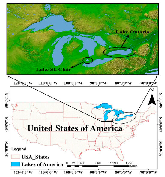
Figure 1.
Location map of Lakes St. Clair and Ontario.
Lake Ontario is the easternmost of the Great Lakes and the smallest in surface area at 19,000 km2. Its maximum length is 311 km, and its maximum width is 85 km. The weather in the Lake Ontario area is marked by sweltering summers, cold winters, and unchanging humidity levels. During the summer season, July usually experiences about 9 h of sunshine each day in the area, with scarce cloud coverage. Moreover, Lake Ontario’s average summer surface water temperature increased by 1.6 degrees Celsius from 1968 to 2002, and the average annual rainfall at Lake St. Clair is 1897.1 mm [16].
The area of Lake St. Clair is 1100 km2 and its average depth is 3.4 m. The lake is fed by the St. Clair River. This is the largest delta of the Great Lakes system. Moreover, the weather changes in this lake include increased mean maximum temperatures, climbing from 16.2 °C in 1989 to 17.5 °C in 2022, showing a rise of 1.3 °C. Over the years, the precipitation trends have changed, resulting in a rise in average yearly rainfall from 1511 mm in 1989 to 1858.8 mm in 2024, an increase of 347.7 mm [17].
In this study, an evaluation of the proposed models was conducted on Lake St. Clair and Lake Ontario utilizing WL time series with high and low variations. The WL variations for both lakes were about 2 m; however, the WL values for Lake St. Clair (about 174–176 m) were higher than those for Lake Ontario (about 74–76 m).
These lakes’ monthly water level (WL) data were collected by the U.S. NOAA from 1918 to 2021. Table 1 indicates the statistical measures of the collected WL data for the two lakes, which were different in the sense of their statistical characteristics. To develop the models, the WL datasets were divided into 80% (1918–2000) for training and 20% (2001–2021) for testing, as shown in Figure 2.

Table 1.
Statistical characteristics of study data.
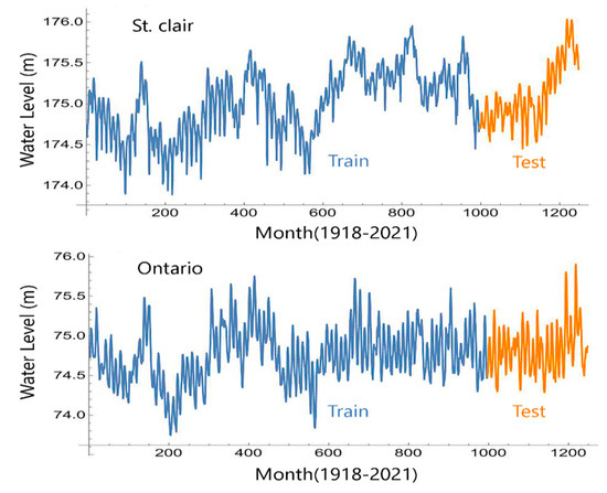
Figure 2.
The time series dataset used for the modeling conducted, including the training and testing covering the years of 1918 to 2021.
Figure 3 indicates that the monthly WL values in Lake St. Clair and Ontario varied over 1918–2021. However, the WL fluctuations for both lakes were similar during the statistical period. Following the partitioning of the datasets, they were normalized between 0 and 1 using their minimum and maximum values, as recommended in previous research [18,19]. Normalization was performed to facilitate convergence during training. It should be noted that the modeling operation was performed with the three mentioned methods in the Mathematica software version 14.
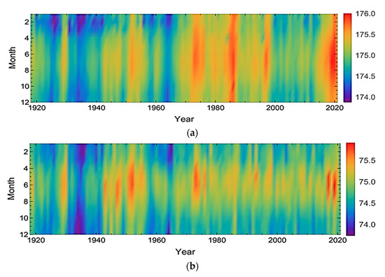
Figure 3.
The monthly water level time series distributed temporally across the years of 1918 to 2021 for Lakes St. Clair (a) and Ontario (b).
2.2. Deep Neural Network Time Series Forecasting Model
2.2.1. Artificial Neural Network (ANN)
One of the supervised ML models, the ANN, falls within the category of artificial intelligence. ANNs were created to generalize mathematical models of biological nervous systems, and the introduction of simplified neurons by McCulloch and Pitts (1943) sparked the initial fascination with neural networks [20]. The brain serves as the inspiration for these computer-based problem-solving tools, known as biological neural networks [21]. ANNs are particularly well suited for the solution of real-world, complex issues, such as comprehending the climate, due to their capacity to generate nonlinear mappings during training [22]. In an ANN model, there are three layers: the input layer, hidden layer, and output layer. The neurons within each layer are connected to all neurons in other layers. ANNs possess the capability to adjust to shifting data patterns and acquire new information, thereby making them highly appropriate for dynamic forecasting environments, and they can handle noisy or incomplete data more effectively than traditional models, leading to more reliable forecasts [23,24]. The representation of the relation between input (x) and output (Y) in an ANN is demonstrated by
The action function is denoted by f, with b representing the bias and Wi denoting the weight of the link. Within a neural system, a weight symbolizes the intensity of a link between two units (or nerve cells). This determines the extent to which a neuron’s output influences another neuron’s input. Figure 4 presents the structure of an ANN model.
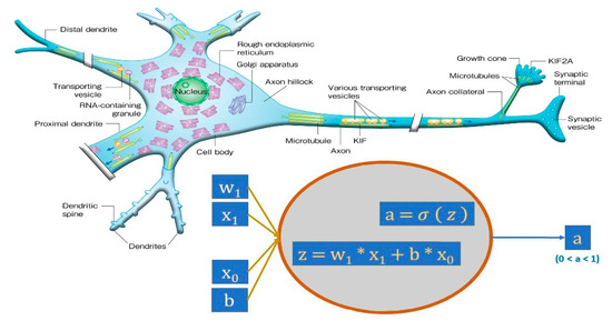
Figure 4.
The structure of a common artificial neural network (ANN) model and biological neuron.
The focus on artificial neural networks has intensified in numerous sectors, especially with regard to forecasting time series data, as they can effectively portray intricate and nonlinear connections. Moreover, as they are able to support both continuous and discrete variables, ANNs are well suited to addressing a broad spectrum of time series forecasting issues.
2.2.2. Deep Learning (DL)
Neural networks incorporated into deep learning facilitate the ability to tackle complex problem-solving challenges. DL, with the implementation of the backpropagation algorithm, can reveal intricate structures in large sets of data to show how a machine should change its internal parameters. This enables the model to compute a representation of each layer from the representation of the previous layer, and the learning of data representations at different levels of abstraction is made possible through the utilization of computational models with multiple processing layers [25]. The ability to uncover patterns and structures within extensive datasets is a defining feature of deep learning methods, particularly deep artificial neural networks. Deep learning networks are characterized by their architectures, which consist of multiple layers of interconnected nodes that enhance prediction and classification. Another of the key strengths of deep learning is its independence of prior data processing, as it automatically extracts and learns features directly from the data [26]. Figure 5 presents the structure of a common DL model.
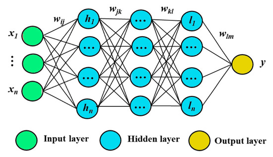
Figure 5.
The structure of a deep learning (DL) model.
The nonlinearity in the network is introduced by the activation function, which also helps it to learn representations and complex patterns [27,28]. Sigmoid, ReLU, Tanh, and Leaky ReLU are some common activation functions. Some popular deep learning algorithms are radial function networks, self-organizing maps, multilayer perceptron, and convolutional neural networks [29]. A flowchart of the steps involved in running an ANN and DL model is shown in Figure 6.
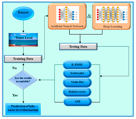
Figure 6.
Flowchart of the artificial neural network and deep learning model.
Sophisticated deep learning algorithms possess adaptability in processing multivariate time series alongside numerous input variables and outputs, additionally being able to extract key features from unprocessed data automatically, thus eliminating the requirement for manual feature engineering.
2.3. Statistical Time Series Forecasting Model
ARIMA Model
ARIMA, a model combining autoregressive integrated moving average components, is an asset in the realm of time series analysis and prediction. ARIMA techniques transform non-stationary data into stationary data through differencing, eliminating trends and seasonality [30]. Due to their effective handling of diverse temporal patterns, ARIMA models are commonly utilized in time series forecasting. In ARIMA models, the parameters are designated as ARIMA (p, d, q), where p corresponds to the order of the autoregressive model and is determined by the number of time lags; the degree of differencing, denoted as d, represents how many past values have been subtracted from the data; and the magnitude of the moving average model is represented by q. Moreover, by adjusting specific parameters to zero, the model can imitate simpler models, like ARMA, AR, I, or MA. The structural components of this model are shown in Figure 7.

Figure 7.
Structural components of autoregressive integrated moving average (ARIMA) model.
Its versatility in capturing complex temporal patterns and adapting to fluctuations in data makes ARIMA a critical tool applied across multiple fields. ARIMA models are capable of capturing trends, seasonality, cycles, and noise in time series data to better understand their complexity and variability. Meanwhile, the importance of ARIMA models in time series forecasting lies in their capability to grasp intricate patterns, adjust to fluctuations, and offer trustworthy predictions.
2.4. Performance Criteria
In this paper, the coefficient of correlation (r), root mean square error (RMSE), and mean absolute percentage error (MAPE) are used to evaluate the performance of the models.
where and represent the observed and predicted values, i is the number of starting terms in the series, N is the number of observations, and and indicate the mean of the observed and predicted values, respectively. Scatter plots and violin plots are employed to visually assess the performance of the models.
3. Results
3.1. Model Development
The division of time series forecasting methods into the univariate and multivariate categories is dependent on the quantity of available variables for observation. Our approach to predicting future WLs involves applying a univariate forecasting method, which operates under the assumption that past values exclusively determine future values in the time series. This strategy’s advantages might surpass those of multivariate time series forecasting. In general, the forecasting of univariate time series tends to be faster than the forecasting of multivariate time series as a result of their lower complexity. Moreover, it is useful in the absence of potential predictors for a target variable forecast. According to previous research [31,32], it has been shown that univariate time series forecasting achieves better accuracy as compared to multivariate forecasting.
The selection of input variables in modeling holds significant importance as it greatly contributes to the model’s effectiveness. Numerous methodologies, including the Gamma Test or principal component analysis [33] and the technique of average mutual information (AMI) [34], can be employed to choose the most suitable input variables for the output variable. Utilizing AMI to select input variables presents a key advantage in its ability to uncover both linear and nonlinear relationships between inputs and outputs, without any preconceived notions about the model’s structure. In contrast to correlation, AMI evaluates the strength of connections beyond linear patterns and quantifies the information content of each input variable concerning the output, providing a means to rank the variables in order of relevance. Due to the fact that, in some areas, it is impossible to measure some variables, single-variable prediction is given priority. In this study, by using a water level parameter and applying the AMI method to determine the appropriate delays, we examine the forecasting operation to evaluate the models.
The value of time delay was determined by employing an autocorrelation function through the implementation of the AMI technique in this study. In Figure 8, the variations in the AMI values for the two lakes are displayed against time. Based on Figure 8, Lakes St. Clair and Ontario both have optimal values for delay, corresponding to a low AMI value of 6. This is marked in the figure with red dots.
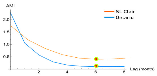
Figure 8.
Average mutual information for Lakes St. Clair and Ontario to determine appropriate delay.
Table 2 illustrates the diverse input variable(s) combinations determined from the AMI results for the prediction of the WLs of both lakes.

Table 2.
The variables used for the multistep-ahead prediction of the lake water level in Lakes St. Clair and Ontario.
During the training phase, the Mathematica software was utilized to determine the optimal parameters of the models by determining the best input combination of the lake WL. The next section will discuss the performance of the two standalone models for each lake individually. In an ARIMA (p, d, q) model, the values for p, d, and q must be integers to accurately determine its structure. Before selecting the optimal ARIMA model for a given time series, one must initially ascertain the appropriate amount of differencing (d) necessary to transform the series into a stationary form and eliminate notable characteristics such as trends or seasonality. When autocorrelated errors persist in the stationary series, incorporating a minimum of one AR term (p ≥ 1) and/or a minimum of one MA term (q ≥ 1) becomes crucial for the forecasting model. In this research, the parameters mentioned for the Lake St. Clair ARIMA (43, 1, 1) and Lake Ontario ARIMA (45, 1, 1) were determined using a walk-forward validation approach. In this way, (i) the data were divided into training and testing sets and (ii) the training set was used to fit the model and then its performance was evaluated in the test set. This process was repeated until the best performance was achieved.
3.2. Results for Lake St. Clair
Statistical and visual analyses were employed to evaluate the performance of the two standalone models, namely machine learning or the ANN and DL, and one statistical model, ARIMA, in forecasting WL values. In this case, the values of the performance criteria, mean absolute percentage error (MAPE), root mean square error (RMSE), and coefficient of correlation (R) were calculated, as indicated in Table 3, for the training and testing periods. In addition, in order to visually evaluate the performance of the models, Taylor diagrams, time series charts, scatter charts, violin charts, and relative error charts of the models are presented for the lakes during the test period.

Table 3.
Performance criteria for the three models in the training and testing periods for Lakes St. Clair and Ontario.
The Taylor diagram serves as a visual aid in assessing how well different models perform by comparing their patterns and statistics with actual data. This thorough visual representation considers three essential statistics, namely the correlation coefficient, RMSE, and standard deviation, in assessing model performance against observations. Therefore, by examining the three mentioned parameters, the models are evaluated together and the model that has the smallest distance from the observed values is selected as the best model. Based on Figure 9, which shows the Taylor diagrams for the ANN and DL models, it can be seen that the ANN-M5 and DL-M4 models, with the lowest error and standard deviation and the highest correlation coefficient, have a smaller difference than the actual values. Therefore, the ANN-M5 and DL-M4 models, with the smallest distance from the observations (0.1269 and 0.1124), perform better than the rest. Moreover, according to Table 3, among the ANN models, the ANN-M5 model performs accurately based on the R (0.956), RMSE (0.2117), and MAPE (0.066) in the testing stage using the W(t), WL(t-1) … WL(t-4) variables. Among the DL models, the DL-M4 model estimates the values with less error based on the greatest value of R (0.990) and lowest value of the RMSE (0.1336) and MAPE (0.067) in the testing stage using the W(t), WL(t-1) … WL(t-3) variables. Regarding the ARIMA models, the ARIMA model estimates with values of R (0.874), RMSE (0.375), and MAPE (0.177) in the testing stage using the W(t), WL(t-1) … WL(t-6) variables, indicating acceptable performance. By comparing the ANN-M5 and ARIMA models with the DL-M4 model, it is found that the DL model surpasses the other models. According to Table 3, the DL model has a lower RMSE and higher R in two scenarios (M3–M4) for Lake St. Clair and in three scenarios (M3–M4–M5) for Lake Ontario in both the testing and training stages. In general, the DL model has a better determination coefficient and an acceptable error rate compared to the other models in most cases.
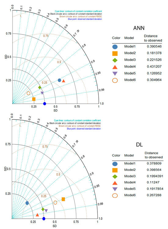
Figure 9.
Taylor diagrams of artificial neural network and deep learning model for Lake St. Clair.
In Figure 10, the best models among the ARIMA, ANN, and DL models (ARIMA, ANN-M5, and DL-M4) are compared with each other. Using complex and powerful models, such as deep neural networks, can lead to overfitting. These models are more capable of learning details and noise and may adapt to noisy details in the training data, instead of learning general patterns. However, according to Figure 10a, each of the models has a limitation in that the DL(M4) model tends to overestimate in some places and the ANN(M5) model tends to underestimate. According to the scatter plots, the DL model stands out as the most accurate model (R2 = 0.980, RMSE = 0.1336), while the ANN model shows a broader distribution of the actual and predicted WLs from line 1:1 (R2 = 0.913, RMSE = 0.2117). However, the ARIMA model, according to the results (R2 = 0.763, RMSE = 0.375), shows a wider distribution. Each of the three types of models, ARIMA, ANN, and DL, exhibits a high level of performance, as indicated by the R2 values, which are between 0.7 and 1 for Lake St. Clair. Figure 10b shows that the relative errors of the ARIMA models are between −1% and 1%, those of the ANN models are roughly between −0.3% and 0.3%, and those of the DL models are roughly between −0.02% and 0.22%. However, the relative errors of most of the forecasted values of the DL model are smaller than those of the other models. As can be seen from the violin plot, the violin shapes of the DL and ANN models are similar to each other and also to the observed one; however, the shape of the DL model is more similar to that of the observed values because of the smaller difference between the maximum (176.04, 176.08), median (175.02, 175.11), and minimum (174.44, 174.55) of the observed and forecasted values. Figure 10c shows the error frequencies of the ARIMA, ANN, and DL models: the mean and standard deviation for ARIMA are (0.0082, 0.220), those for the ANN are (0.0807, 0.116), and those for the DL models are (−0.117, 0.064). Therefore, it can be deduced that the deep learning model exhibits greater proficiency in estimating the WL(t) in Lake St. Clair compared to the ANN and ARIMA models.
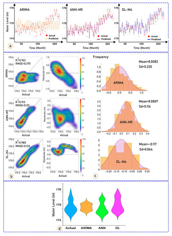
Figure 10.
Time series graphs (a), scatter plots and relative error metric (b), frequencies of error values (c), and violin plots (d) of the actual and predicted WL(t) for the three models for Lake St. Clair at the testing stage.
3.3. Results for Lake Ontario
For Lake Ontario, the performance of the three models (ARIMA, ANN, and DL) was also compared using the statistical and visual approaches. Table 3 shows the performance criteria of the models in the training and testing phases. It indicates that ARIMA (R = 0.876, RMSE = 0.306, and MAPE = 0.37), ANN-M6 (R = 0.912, RMSE = 0.146, and MAPE = 0.072), and DL-M3 (R = 0.952, RMSE = 0.1257, and MAPE = 0.057) outperform the other ARIMA, ANN, and DL models using six and three input variables, respectively. Most DL models estimate the WL(t) values more accurately than the ANN and the ARIMA models in both the training and testing periods. Moreover, according to Figure 11, which shows the Taylor diagrams for Lake Ontario, the ANN-M6 and DL-M3 models have a smaller distance from the observations than the other scenarios (0.1904, 0.1185) and therefore include more accurate predictions.
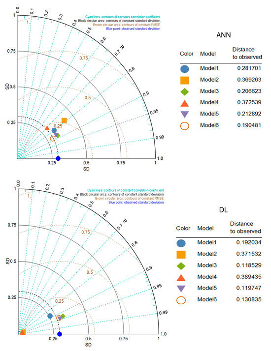
Figure 11.
Taylor diagrams of artificial neural network and deep learning model for Lake Ontario.
Figure 12a–d show the time series plots, scatter (1:1) plots, violin plots, and relative error diagrams of the best three models (M6 and M3) for Lake Ontario. Figure 12a shows that, during the testing period, the ARIMA, DL (M3), and ANN (M6) models give accurate results and values close to the observed WL(t). Examining the scatter plot data (Figure 12b), the DL model is the most precise (R2 = 0.906, RMSE = 0.1257), while the ANN model exhibits a substantial discrepancy in predicting the water levels from reality (R2 = 0.831, RMSE = 0.1460) and the ARIMA model (R2 = 0.756, RMSE = 0.306). Figure 12b indicates that the ranges of the relative errors for the ARIMA, ANN, and DL models are almost the same, i.e., (−1, 1), (−0.5 to 0.5), and (−0.4 to 0.4). However, the majority of the forecasted values of the DL-M3 model have a smaller error than those of the other models. Based on the violin plot (Figure 12d), the violin shape of the DL model is more similar to the shape of the observed WL(t) values than the shapes of the ANN and ARIMA models, due to the similar values of the maximum (75.91 and 76.41), median (74.82, 73.31), and minimum (74.28, 73.15) criteria. Figure 12c shows that the error frequency, mean, and standard deviation for the ARIMA, ANN, and DL models are (0.0950, 0.4614), (−0.0039, 0.2224), and (−0.0203, 0.1240). In general, based on the WL(t) forecasts, it can be inferred that both of the intelligent models’ performance is outstanding and they deserve recognition as they exhibit excellent results (0.7 < R2 ≤ 1.0); however, the DL model shows somewhat greater accuracy in its results compared to the ARIMA and ANN techniques in estimating the WL(t) in Lake Ontario.
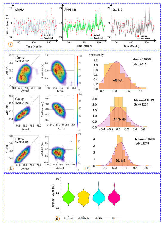
Figure 12.
Time series graphs (a), scatter plots and relative errors (b), error frequency values (c), and violin plots (d) of the actual and predicted WL(t) for the three models for Lake Ontario at the testing stage.
4. Discussion
To summarize, affordable data-driven approaches like ANNs, deep learning, and ARIMA excel in handling immense datasets and reflecting evolving hydrological situations. The DL model displayed impressive accuracy in predicting the WL, particularly regarding extreme values, such as the maximum and minimum levels. Based on the statistical indicators and diverse graphical representations, the DL model displayed superior performance compared to the ARIMA and ANN models when forecasting the lake water levels. Through the implementation of ensemble learning, the DL technique reduces overfitting by enhancing the model stability through increased precision and reduced variance. Some advantages of DL are as follows: (i) DL has good exploitation capabilities; (ii) it is easy to implement and understand; (iii) it does not require excessive calculations; (iv) and it has a greater ability to find the optimal results in a unimodal fashion. The only limitation of DL is its overfitting, which occurs when a model is too complex. According to the time series in the ARIMA model, it is clear that this model cannot follow the data trends in both lakes and only considers the changes around the beginning. For this reason, the ARIMA model in this study had weak performance compared to the other models. In order to improve the predictions in the ARIMA model, the trends can be removed before fitting the model and then added again, but this was beyond the scope of this study.
The results of this study are in accordance with prior investigations [4,5,12,35] in which a DL model was found to significantly increase the accuracy. A significant and notable aspect is that the standalone DL model has less been investigated and evaluated in estimating the WLs of lakes in the United States. The authors in [36] applied the gated recurrent unit (GRU), long short-term memory (LSTM), and temporal convolutional network (TCN) to predict WLs for different forecast periods at five stations at Poyang Lake. In 80% of the forecast scenarios, the lake WL prediction accuracy of BMA displayed a noticeable enhancement in the metrics of R2 and NSE, consistently ranking among the top two in all forecast scenarios. The framework proposed in their study achieves high WL forecast accuracy without the need for the intricate comparison and selection of DL models, making it applicable to the prediction of various hydrological variables as well. In another study, [7], by means of Gaussian process regression (GPR), minimax probability machine regression (MPMR), relevance vector machine (RVM), and extreme learning machine (ELM) models, the fluctuations in the water levels across Lakes Michigan, Superior, Huron, Ontario, and Erie in the United States were projected. The results of this work indicated that the minimax probability machine regression model (R2 = 0.984, MAE = 0.035, and RMSE = 0.044) generated more reliable projections of the lake water levels than the competing models. In another study [37], the authors employed the MARS, M5-Tree, and LSSVR approaches to forecast the water levels of Lakes Superior, Ontario, Erie, Huron, and Michigan, located in the northern region of the United States. Compared with other models, the LSSVR model yielded more promising outcomes.
Numerous past studies have shown that deep learning models are more trustworthy than standalone models with regard to forecasting lake water levels, thanks to their complex and nonlinear characteristics, which give them a competitive edge [38,39,40,41]. The objective of deep learning models is to acquire knowledge from extensive datasets in order to detect patterns and connections that can be utilized for precise prediction or classification.
Metaheuristic-based ML models have been shown in this study to be capable of achieving significant gains and, overall, are more desirable than traditional models due to their potential. Moreover, upon examining the data gathered from the two different lakes, it becomes evident that the calculations of the water levels for Lake Ontario are more precise compared to those for Lake St Clair. The dissimilarity in the statistical characteristics between the two lakes is the reason for this.
5. Conclusions
The application of ML techniques is greatly beneficial with regard to producing accurate predictions of nonlinear processes, specifically in the case of the lake water level (WL), which exhibits complex behavior and is influenced by various factors, such as rainfall and evaporation. In the present research, the ability of two ML models (i.e., ANN with DL) and a statistical model (ARIMA) to forecast the WL(t) for Lakes St. Clair and Ontario was assessed. AMI, a nonlinear input variable selection method, was used to identify the most influential inputs for the modeling process in preparation. This method considered various lag times of the lake WL up to a maximum lag of 6 months. By considering statistical indicators including the sample correlation coefficient, r, MAPE, and RMSE, along with examining statistical graphs, an evaluation was performed on the performance of the two built models. According to the findings, the ML models created for both lakes displayed impressive performance. For Lake St. Clair, the models showed slightly more errors in their results. Comparatively, the DL model demonstrated superior performance in predicting extreme water levels for both lakes, surpassing the abilities of the ANN and ARIMA models. In simpler terms, the DL model proved to be an exceptional forecasting tool with remarkable abilities to precisely produce WL time series.
To improve the structure of intelligent standalone models, it is essential for future research to focus on the utilization of DL and counterpart hybrid methods to predict additional hydrological variables, while also conducting comparisons with other algorithms. Based on the successful implementation of a univariate model for lake WL forecasting in this study, the incorporation of other potential variables (e.g., temperature, precipitation, humidity) is recommended to develop a multivariate forecasting model for lake water levels. It is further suggested to apply the models to simulate the WLs of other surface water bodies, including rivers, dams, and aquifer media.
The performance of the models relies on the quality of the data employed during training, and their training capabilities may be restricted by limitations in data availability. Therefore, by replacing the data on incomplete years in the form of interpolation or using other methods, a longer period of time can be considered and the water level trend can be carefully examined. Achieving peak performance in deep learning models necessitates the meticulous adjustment of the hyperparameters, which may be time-consuming and may not consistently lead to the optimal model for a particular application, thus limiting their predictive capabilities. Moreover, it is necessary to solve the problems of overfitting and underfitting with specific skills and by using the most important layers in these models.
Author Contributions
Conceptualization, W.A.H.A.-N., L.A.-j.D. and S.G.; methodology, W.A.H.A.-N., S.G. and B.M.G.K.; software, S.G. and L.A.-j.D.; validation, B.M.G.K. and S.G.; formal analysis, W.A.H.A.-N. and L.A.-j.D.; investigation, S.G.; resources, B.M.G.K.; data curation, S.G. and W.A.H.A.-N.; writing—original draft preparation, S.G., L.A.-j.D., W.A.H.A.-N. and B.M.G.K.; writing—review and editing, B.M.G.K. and S.G.; visualization, S.G.; supervision, W.A.H.A.-N.; project administration, L.A.-j.D.; funding acquisition, W.A.H.A.-N. All authors have read and agreed to the published version of the manuscript.
Funding
This research received no external funding.
Data Availability Statement
The data used in this study will be available upon reasonable request.
Acknowledgments
We are grateful to all anonymous reviewers and academic editors for their valuable comments and suggestions, which significantly contributed to enhancing the quality and presentation of the paper.
Conflicts of Interest
The authors declare no conflicts of interest.
References
- Khatibi, R.; Ghorbani, M.A.; Naghshara, S.; Aydin, H.; Karimi, V. A framework for ‘Inclusive Multiple Modelling’ with critical views on modelling practices–Applications to modelling water levels of Caspian Sea and Lakes Urmia and Van. J. Hydrol. 2020, 587, 124923. [Google Scholar] [CrossRef]
- Yadav, B.; Eliza, K. A Hybrid Wavelet-Support Vector Machine model for Prediction of Lake water level Fluctuations Using Hydro-Meteorological Data. Measurement 2017, 103, 294–301. [Google Scholar] [CrossRef]
- Khatibi, R.; Ghorbani, M.A.; Naghipour, L.; Jothiprakash, V.; Fathima, T.A.; Fazelifard, M.H. Inter-comparison of time series models of lake levels predicted by several modeling strategies. J. Hydrol. 2014, 511, 530–545. [Google Scholar] [CrossRef]
- Zhu, S.; Lu, H.; Ptak, M.; Dai, J.; Ji, Q. Lake water-level fluctuation forecasting using machine learning models: A systematic review. Environ. Sci. Pollut. Res. 2020, 27, 44807–44819. [Google Scholar] [CrossRef] [PubMed]
- Zhu, S.; Hrnjica, B.; Ptak, M.; Choiński, A.; Sivakumar, B. Forecasting of water level in multiple temperate lakes using machine learning models. J. Hydrol. 2020, 585, 124819. [Google Scholar] [CrossRef]
- Kisi, O.; Shiri, J.; Nikoofar, B. Forecasting daily lake levels using artificial intelligence approaches. Comput. Geosci. 2012, 41, 169–180. [Google Scholar] [CrossRef]
- Bonakdari, H.; Ebtehaj, I.; Samui, P.; Gharabaghi, B. Lake water-level fluctuations forecasting using minimax probability machine regression, relevance vector machine, gaussian process regression, and extreme learning machine. Water Resour. Manag. 2019, 33, 3965–3984. [Google Scholar] [CrossRef]
- Nhu, V.H.; Shahabi, H.; Nohani, E.; Shirzadi, A.; Al-Ansari, N.; Bahrami, S.; Miraki, S.; Geertsema, M.; Nguyen, H. Daily Water Level Prediction of Zrebar Lake (Iran): A Comparison between M5P, Random Forest, Random Tree and Reduced Error Pruning Trees Algorithms. ISPRS Int. J. Geo-Inf. 2020, 9, 479. [Google Scholar] [CrossRef]
- Pan, M.; Zhou, H.; Cao, J.; Liu, Y.; Hao, J.; Li, S.; Chen, C. Water Level Prediction Model Based on GRU and CNN. IEEE Access 2020, 8, 60090–60100. [Google Scholar] [CrossRef]
- Choi, C.; Kim, J.; Han, H.; Han, D.; Kim, H.S. Development of Water Level Prediction Models Using Machine Learning in Wetlands: A Case Study of Upo Wetland in South Korea. Water 2020, 12, 93. [Google Scholar] [CrossRef]
- Ahmed, A.N.; Yafouz, A.; Birima, A.H.; Kisi, O.; Huang, Y.F.; Sherif, M.; Sefelnasr, A.; El-Shafie, A. Water level prediction using various machine learning algorithms: A case study of Durian Tunggal river, Malaysia. Eng. Appl. Comput. Fluid Mech. 2022, 16, 422–440. [Google Scholar] [CrossRef]
- Atashi, V.; Gorji, H.T.; Shahabi, S.M.; Kardan, R.; Lim, Y.H. Water level forecasting using deep learning time-series analysis: A case study of red river of the north. Water 2022, 14, 1971. [Google Scholar] [CrossRef]
- Pang, G.; Shen, C.; Cao, L.; Hengel, A.V.D. Deep learning for anomaly detection: A review. ACM Comput. Surv. (CSUR) 2021, 54, 1–38. [Google Scholar] [CrossRef]
- Cremer, C.Z. Deep limitations? Examining expert disagreement over deep learning. Prog. Artif. Intell. 2021, 10, 449–464. [Google Scholar] [CrossRef]
- Picon, A.; Alvarez-Gila, A.; Irusta, U.; Echazarra, J. Why deep learning performs better than classical machine learning? Dyna Ing. E Ind. 2020, 95, 119–122. [Google Scholar] [CrossRef] [PubMed]
- Dove-Thompson, D.; Lewis, C.; Gray, P.A.; Chu, C.; Dunlop, W.I. A Summary of the Effects of Climate Change on Ontario’s Aquatic Ecosystems. 2011. Available online: https://www.cabidigitallibrary.org/doi/full/10.5555/20173382427 (accessed on 28 April 2024).
- Lee, D.H.; Moulton, R.; Hibner, B.A. Climate Change Impacts on Western Lake Erie, Detroit River, and Lake St. Clair Water Levels; Environment Canada, Atmospheric Environment Service: Toronto, ON, Canada, 1996. [Google Scholar]
- Ghorbani, M.A.; Deo, R.C.; Karimi, V.; Yaseen, Z.M.; Terzi, O. Implementation of a hybrid MLP-FFA model for water level prediction of Lake Egirdir, Turkey. Stoch. Environ. Res. Risk Assess. 2018, 32, 1683–1697. [Google Scholar] [CrossRef]
- Abraham, A. Artificial neural networks. In Handbook of Measuring System Design; Wiley: Hoboken, NJ, USA, 2005. [Google Scholar]
- Tran, T.T.K.; Bateni, S.M.; Ki, S.J.; Vosoughifar, H. A review of neural networks for air temperature forecasting. Water 2021, 13, 1294. [Google Scholar] [CrossRef]
- Elsner, J.B.; Tsonis, A.A. Nonlinear prediction, chaos, and noise. Bull. Am. Meteorol. Soc. 1992, 73, 49–60. [Google Scholar] [CrossRef]
- Wu, Y.C.; Feng, J.W. Development and application of artificial neural network. Wirel. Pers. Commun. 2018, 102, 1645–1656. [Google Scholar] [CrossRef]
- Zhang, G.; Patuwo, B.E.; Hu, M.Y. Forecasting with artificial neural networks: The state of the art. Int. J. Forecast. 1998, 14, 35–62. [Google Scholar] [CrossRef]
- LeCun, Y.; Bengio, Y.; Hinton, G. Deep learning. Nature 2015, 521, 436–444. [Google Scholar] [CrossRef] [PubMed]
- Rusk, N. Deep learning. Nat. Methods 2016, 13, 35. [Google Scholar] [CrossRef]
- Luhaniwal, V. Forward propagation in neural networks–Simplified math and code version. Towards Data Sci. 2019, 6, 112–120. [Google Scholar]
- Krogh, A. What are artificial neural networks? Nat. Biotechnol. 2008, 26, 195–197. [Google Scholar] [CrossRef]
- Biswal, A. Top 10 Deep Learning Algorithms You Should Know in 2021. 2021. Available online: https://www.simplilearn.com/tutorials/deep-learning-tutorial/deep-learning-algorithm (accessed on 26 May 2024).
- Lai, Y.; Dzombak, D.A. Use of the autoregressive integrated moving average (ARIMA) model to forecast near-term regional temperature and precipitation. Weather Forecast. 2020, 35, 959–976. [Google Scholar] [CrossRef]
- Iwok, I.A.; Okpe, A.S. A comparative study between univariate and multivariate linear stationary time series models. Am. J. Math. Stat. 2016, 6, 203–212. [Google Scholar]
- Castán-Lascorz, M.A.; Jiménez-Herrera, P.; Troncoso, A.; Asencio-Cortés, G. A new hybrid method for predicting univariate and multivariate time series based on pattern forecasting. Inf. Sci. 2022, 586, 611–627. [Google Scholar] [CrossRef]
- Noori, R.; Karbassi, A.R.; Moghaddamnia, A.; Han, D.; Zokaei-Ashtiani, M.H.; Farokhnia, A.; Gousheh, M.G. Assessment of input variables determination on the SVM model performance using PCA, Gamma test, and forward selection techniques for monthly stream flow prediction. J. Hydrol. 2011, 401, 177–189. [Google Scholar] [CrossRef]
- Ghorbani, M.; Kahya, E.; Ruskeepää, H.; Roshni, T.; Kashani, M.H.; Karimi, V.; Arikan, B.B. Temporal connections in reconstructed monthly rainfall time series in different rainfall regimes of Turkey. Arab. J. Geosci. 2022, 15, 1015. [Google Scholar] [CrossRef]
- Zakaria, M.N.A.; Ahmed, A.N.; Malek, M.A.; Birima, A.H.; Khan, M.M.H.; Sherif, M.; Elshafie, A. Exploring machine learning algorithms for accurate water level forecasting in Muda river, Malaysia. Heliyon 2023, 9, E17689. [Google Scholar] [CrossRef]
- Li, G.; Liu, Z.; Zhang, J.; Han, H.; Shu, Z. Bayesian model averaging by combining deep learning models to improve lake water level prediction. Sci. Total Environ. 2024, 906, 167718. [Google Scholar] [CrossRef] [PubMed]
- Demir, V.; Yaseen, Z.M. Neurocomputing intelligence models for lakes water level forecasting: A comprehensive review. Neural Comput. Appl. 2023, 35, 303–343. [Google Scholar] [CrossRef]
- Wen, J.; Han, P.F.; Zhou, Z.; Wang, X.S. Lake level dynamics exploration using deep learning, artificial neural network, and multiple linear regression techniques. Environ. Earth Sci. 2019, 78, 222. [Google Scholar] [CrossRef]
- Barzegar, R.; Adamowski, J.; Quilty, J.; Taghi Aalami, M. Using a boundary-corrected wavelet transform coupled with machine learning and hybrid deep learning approaches for multi-step water level forecasting in Lakes Michigan and Ontario. In Proceedings of the 22nd EGU General Assembly, Online, 4–8 May 2020; p. 4233. [Google Scholar]
- Yue, L.; Zan, F.; Liu, X.; Yuan, Q.; Shen, H. The spatio-temporal reconstruction of lake water levels using deep learning models: A case study on Altai mountains. IEEE J. Sel. Top. Appl. Earth Obs. Remote Sens. 2022, 15, 4919–4940. [Google Scholar] [CrossRef]
- Ozdemir, S.; Ozkan Yildirim, S. Prediction of Water Level in Lakes by RNN-Based Deep Learning Algorithms to Preserve Sustainability in Changing Climate and Relationship to Microcystin. Sustainability 2023, 15, 16008. [Google Scholar] [CrossRef]
- Herath, M.; Jayathilaka, T.; Hoshino, Y.; Rathnayake, U. Deep machine learning-based water level prediction model for Colombo flood detention area. Appl. Sci. 2023, 13, 2194. [Google Scholar] [CrossRef]
Disclaimer/Publisher’s Note: The statements, opinions and data contained in all publications are solely those of the individual author(s) and contributor(s) and not of MDPI and/or the editor(s). MDPI and/or the editor(s) disclaim responsibility for any injury to people or property resulting from any ideas, methods, instructions or products referred to in the content. |
© 2024 by the authors. Licensee MDPI, Basel, Switzerland. This article is an open access article distributed under the terms and conditions of the Creative Commons Attribution (CC BY) license (https://creativecommons.org/licenses/by/4.0/).