Reaeration Coefficient Empirical Equation Selection for Water Quality Modeling in Surface Waterbodies: An Integrated Numerical-Modeling-Based Technique with Field Case Study

Abstract

Empirical equations were developed by many investigators to determine the reaeration coefficients (Ka) required for predicting dissolved oxygen concentrations (DO) in surface waters, especially rivers, lakes, and reservoirs. However, these equations yield a wide range of Ka values. In this paper, an integrated numerical-modeling-based technique was developed to check the validity of the equations before using them in water quality modeling for rivers, lakes, and reservoirs. Depending on direct field measurements at the Hilla River headwater (Saddat Al-Hindiyah Reservoir, Iraq), the temporal oxygen mass transport at the water surface was estimated numerically by solving the one-dimensional advection diffusion equation and then using each Ka empirical equation separately in the numerical model obtained the best specific-waterbody equation. The DO modeling results showed that using a reservoir reaeration coefficient of 0.1 day⁻¹ at 20 °C predicts the best DO simulation with low MAEs of 0.4987 and 0.7880 mg/L during the study years 2021 and 2022, respectively, compared to the field data. However, using the Ka empirical equations simulates the DO with wide-ranging statistical errors even though the temporal Ka values have a similar trend during the year. It was noticed that the empirical equations produced maximum Ka values of (0.0080–0.0967 day⁻¹) and minimum Ka values of (0.00052–0.0267 day⁻¹) in 2021 and maximum Ka values of (0.0079 to 0.0951 day⁻¹) and minimum Ka values of (0.00012 and 0.0231 day⁻¹) in 2022. The present equation selection technique revealed that Broecker et al.’s equation followed by Smith’s equation, developed in 1978, are the best selection for water quality modeling at the Hilla River headwater (MAEs: 0.1347 and 0.1686 mg/L in 2021, respectively; and MAEs: 0.1400 and 0.1744 mg/L in 2022, respectively). Hence, it is necessary to find good agreement for the equation-based prediction of DO, DO source–sink, and Ka values compared to the validated model before making selection.

1. Introduction

The oxygen exchange at the air–water interface in surface waterbodies is important for managing water quality constituents, especially dissolved oxygen; therefore, this exchange has received much attention in water quality modeling [1,2]. The rate at which oxygen transfers from air to water is known as the reaeration rate. Hence, the well-defined reaeration rate value, usually measured by the reaeration coefficient (Ka), plays a major role in estimating the dissolved oxygen concentrations (DO). To explain this oxygen reaeration process mathematically, two theories have been developed [1]: the surface renewal theory and the two-film theory. However, it is difficult and time consuming to estimate the theoretical parameters required to determine reaeration coefficient for every water quality modeling case study. Accordingly, most studies have employed empirical methods to determine the reaeration coefficient based on laboratory and/or field investigations [3]. Many Ka empirical equations have been used to simulate the dissolved oxygen reaeration process in surface water quality modeling. Since each Ka empirical equation was developed originally for a specific waterbody and depending on a specific approach, applying different Ka empirical equations on another particular study area leads to different Ka values with different precisions compared to field data [4,5,6].

The Ka equation can be developed in lab or in field separately or instantaneously along with DO measurements. Ref. [7] studied the reaeration induced by wind speed and stream flow experimentally for Ka determination purposes. In the laboratory, the wind speed over the water surface was measured by a thermal anemometer with a hot film sensor. Under a variety of wind conditions, the wind speed, stream flow characteristics, and oxygen transport rates were measured. Regressing the wind speeds and Ka values showed that all measured reaeration coefficient values increased with increasing wind speed, and the rate of increase was much faster at a high wind speed than at a low wind speed. Wind can enhance the DO transfer process in slow stream flows even at low wind speeds, but it does not show a significant effect on Ka values for pure shear driven flow such as fast streams. As a result, the waterbody’s forcing flow mechanisms must be recognized to determine the dominant one (wind or shear driven flow). One experimental and analytical approach can be used to select the best empirical equation of Ka determination was addressed by [8]. The approach developed a novel equation to estimate the reaeration coefficient. The determination process involved finding Ka by making DO mass balance over time within a manufactured circular hydraulic channel and then linking the predicted Ka values with the flow physical and hydraulic parameters using the dimensional analysis. In this study, the relationship between the surface flow and the root mean square of the free surface’s vertical velocity yielded a new dimensionless number input in addition to the traditional parameters used to determine Ka such as water depth and velocity. By comparing the developed equation to the available prediction equations of Ka, the applicable equation can be specified. Even though this approach leads to a new empirical equation, the equation would be applied to a specific waterbody, where the equation is developed, and needs to be calibrated before any further implementation to account for the DO temporal variability.

For Ka determinations in rivers, Ref. [9] carried out a comparative analysis based on different empirical equations to determine the reaeration rate of the Otamiri and Kaduna Rivers, Imo State, Nigeria. Different reaeration rate equations were applied to find the suitable one for each river without linking DO and Ka instantaneously. The selected equations included O’Connor, Parkhurst and Pomeroy, Dobbins, Krenkel, Churchil, Owens, and Thackston. The reaeration coefficient was calculated using data collected from the both rivers, giving seven Ka values ranged from 0.0000.362 to 0.354 day⁻¹ for the Otamiri River and other seven values ranged from 0.141 to 4.32 day⁻¹ for the Kaduna River. Selecting the right Ka value of the river was carried out by making comparisons with previous works. The past calculated Ka value for the Otamiri River (0.0753 day⁻¹) agreed with the O’Connor’s equation, while the Ka value for the Kaduna river (0.954 day⁻¹) agreed with the Parkhurst and Pomeroy equation. The results indicated that the reaeration equations of O’Connor and Parkhurst and Pomeroy are the most reliable among the other equations. Hence, these two equations can be used to predict the reaeration coefficient theoretically without the need to go through the stage of hard laboratory tests. However, such a procedure of calculating the Ka value in surface waterbodies (rivers, lakes, or reservoirs) ignores the seasonality effect alongside the instantaneous variation of DO. Hence, the predicted Ka values cannot be used for real case studies, which are unsteady, and the same study must be performed again whenever there is a need to determine Ka. Similarly, Ref. [10] reviewed several reaeration coefficient empirical equations that are wind-based (scaled to 10 m above the water surface) and developed using various methods for lakes and reservoirs. All of these equations were built under specific conditions at 20 °C. The main differences between methods are space and time coverage. In this research, a new wind-based model was developed in which extra variables describing the spatial coverage of the reaeration coefficient estimates and lake size had a significant effect on the relationship between wind speed and lake size. The outcomes highlighted potential limitations when using wind-based models to predict reaeration coefficients across lakes with proper prediction errors or directly measure reaeration coefficients in the field whenever possible. The key finding is that choosing the appropriate Ka equation confines the Ka prediction errors. For more detailed discussions about the wind-based equations, many of them were listed in [11].

Another interesting approach is that of [12]. The reaeration coefficients were determined for Onondaga Lake, New York, from temporal direct observations of DO concentrations during the 1989 and 1990 post-turnover recovery periods. During the sampling period, the lake was well mixed vertically and displayed a slight variation in DO with depth. In this approach, the DO mass balance was utilized to calculate the reaeration coefficients by assuming a constant net DO sink term and variable DO reaeration source–sink term over the study period of each year. Fitting the observed DO concentrations showed that the temporal values of Ka at 20 °C were 0.22 day⁻¹ and 0.13 day⁻¹ in 1989 and 1990, respectively. Also, comparisons were made with other wind-based empirical equations of calculating Ka. The approach performed well in determining the Ka values and DO concentrations over the short period of time where Ka is almost constant or average. Thus, applying the approach to a long time scale may be appropriate.

Concerning the above reaeration coefficient determination approaches, it is necessary to determine the appropriate Ka values that simulate the DO concentrations in surface waterbodies efficiently during the study period. Therefore, this research aims to apply a new approach to select the best available empirical equation of Ka numerically. In addition, the dissolved oxygen concentrations along with the reaeration coefficient values can be simulated with time based on field measurements of DO and temperature. Hence, this approach provides a general way to choose the best Ka determination equation for water quality modeling purposes based on direct field measurements.

2. Methodology

2.1. Conceptual Framework of the Study

A general conceptual framework, applied in this research, for selecting the appropriate Ka equation for surface waterbodies modeling is shown in Figure 1. To solve the governing and auxiliary equations, a DO numerical model was developed to simulate the DO temporal variation. The procedure starts by calculating the Ka values from any applicable empirical equation, depending on the waterbody system type (river, lake, or reservoir), and then the DO numerical model is run over time based on the calculated Ka values. Different Ka equations are used to achieve the best matching between the DO numerical predictions and field measurements with less statistical errors, the root mean squared error (RMSE), and the mean absolute error (MAE).

The framework was applied to select the Ka equation that is more applicable to simulate the DO concentrations of Hilla River headwater at Saddat Al-Hindiyah Reservoir, Iraq. Hence, all Ka empirical equations are a function of wind speed (W) and water depth (H) as depicted in Table 1 since the study area water system, which is a reservoir, has stagnant water conditions and different from river systems [12,13,14,15,16,17,18].

Table 1. Lake and reservoir Ka empirical equations at 20 °C, where H is the water depth (m), and W is the wind speed at 10 m height above the water surface (m/s).

Equation of Ka	Equation Reference	Equation No.
$\mathrm{K}\mathrm{a}=[0.0276({\mathrm{W}}^2)]/\left[\mathrm{H}\right]$	Downing and Truesdale (1955)	(1)
$\mathrm{K}\mathrm{a}=[0.64+(0.128{\mathrm{W}}^2)]/\left[\mathrm{H}\right]$	Smith (1978)	(2)
$\mathrm{K}\mathrm{a}=\left[\mathrm{\alpha }{\mathrm{W}}^{\mathrm{\beta }}\right]/\left[\mathrm{H}\right]$ $\mathrm{a}\mathrm{t} \mathrm{W}<3.5 \mathrm{m}/\mathrm{s},\mathrm{\alpha }=0.2,\mathrm{\beta }=1$ $\mathrm{K}\mathrm{a}=\left[\mathrm{\alpha }{\mathrm{W}}^{\mathrm{\beta }}\right]/\left[\mathrm{H}\right]$ $\mathrm{a}\mathrm{t} \mathrm{W}>3.5 \mathrm{m}/\mathrm{s},\mathrm{\alpha }=0.057,\mathrm{\beta }=2$	Gelda et al. (1996)	(3)
$\mathrm{K}\mathrm{a}=[0.0432({\mathrm{W}}^2)]/\left[\mathrm{H}\right]$	Kanwisher (1963)	(4)
$\mathrm{K}\mathrm{a}=\left[0.362\left({\mathrm{W}}^{0.5}\right)\right]/\left[\mathrm{H}\right]$ $\mathrm{a}\mathrm{t} \mathrm{W}<5.5 \mathrm{m}/\mathrm{s}$ $\mathrm{K}\mathrm{a}=\left[0.0277\left({\mathrm{W}}^2\right)\right]/\left[\mathrm{H}\right]$ $\mathrm{a}\mathrm{t} \mathrm{W}>5.5 \mathrm{m}/\mathrm{s}$	Banks (1975)	(5)
$\mathrm{K}\mathrm{a}=[0.5+(0.05{\mathrm{W}}^2)]/\left[\mathrm{H}\right]$	Cole and Buchak (1995)	(6)
$\mathrm{K}\mathrm{a}=\left[0.156\left({\mathrm{W}}^{0.63}\right)\right]/\left[\mathrm{H}\right]$ $\mathrm{a}\mathrm{t} \mathrm{W}\le 4.1 \mathrm{m}/\mathrm{s}$ $\mathrm{K}\mathrm{a}=[0.0269({\mathrm{W}}^{1.9})]/\left[\mathrm{H}\right]$ $\mathrm{a}\mathrm{t} \mathrm{W}>4.1 \mathrm{m}/\mathrm{s}$	Liss (1973)	(7)
$\mathrm{K}\mathrm{a}=\left[0.139\mathrm{W}\right]/\left[\mathrm{H}\right]$	Yu et al. (1977)	(8)
$\mathrm{K}\mathrm{a}=\left[0.398\mathrm{W}\right]/\left[\mathrm{H}\right]$ $\mathrm{a}\mathrm{t} \mathrm{W}<1.6 \mathrm{m}/\mathrm{s}$ $\mathrm{K}\mathrm{a}=[0.155{(\mathrm{W}}^2)]/[\mathrm{H}]$ $\mathrm{a}\mathrm{t} \mathrm{W}\ge 1.6 \mathrm{m}/\mathrm{s}$	Weiler (1974)	(9)
$\mathrm{K}\mathrm{a}=\left[0.864\mathrm{W}\right]/\left[\mathrm{H}\right]$	Broecker et al. (1978)	(10)
$\mathrm{K}\mathrm{a}=\left[0.0986\left({\mathrm{W}}^{1.64}\right)\right]/\left[\mathrm{H}\right]$	Wanninkhof et al. (1991)	(11)
$\mathrm{K}\mathrm{a}=\left[0.864\mathrm{W}\right]/\left[\mathrm{H}\right]$	Banks and Herrera (1977)	(12)

Table 1. Lake and reservoir Ka empirical equations at 20 °C, where H is the water depth (m), and W is the wind speed at 10 m height above the water surface (m/s).

Equation of Ka	Equation Reference	Equation No.
$\mathrm{K}\mathrm{a}=[0.0276({\mathrm{W}}^2)]/\left[\mathrm{H}\right]$	Downing and Truesdale (1955)	(1)
$\mathrm{K}\mathrm{a}=[0.64+(0.128{\mathrm{W}}^2)]/\left[\mathrm{H}\right]$	Smith (1978)	(2)
$\mathrm{K}\mathrm{a}=\left[\mathrm{\alpha }{\mathrm{W}}^{\mathrm{\beta }}\right]/\left[\mathrm{H}\right]$ $\mathrm{a}\mathrm{t} \mathrm{W}<3.5 \mathrm{m}/\mathrm{s},\mathrm{\alpha }=0.2,\mathrm{\beta }=1$ $\mathrm{K}\mathrm{a}=\left[\mathrm{\alpha }{\mathrm{W}}^{\mathrm{\beta }}\right]/\left[\mathrm{H}\right]$ $\mathrm{a}\mathrm{t} \mathrm{W}>3.5 \mathrm{m}/\mathrm{s},\mathrm{\alpha }=0.057,\mathrm{\beta }=2$	Gelda et al. (1996)	(3)
$\mathrm{K}\mathrm{a}=[0.0432({\mathrm{W}}^2)]/\left[\mathrm{H}\right]$	Kanwisher (1963)	(4)
$\mathrm{K}\mathrm{a}=\left[0.362\left({\mathrm{W}}^{0.5}\right)\right]/\left[\mathrm{H}\right]$ $\mathrm{a}\mathrm{t} \mathrm{W}<5.5 \mathrm{m}/\mathrm{s}$ $\mathrm{K}\mathrm{a}=\left[0.0277\left({\mathrm{W}}^2\right)\right]/\left[\mathrm{H}\right]$ $\mathrm{a}\mathrm{t} \mathrm{W}>5.5 \mathrm{m}/\mathrm{s}$	Banks (1975)	(5)
$\mathrm{K}\mathrm{a}=[0.5+(0.05{\mathrm{W}}^2)]/\left[\mathrm{H}\right]$	Cole and Buchak (1995)	(6)
$\mathrm{K}\mathrm{a}=\left[0.156\left({\mathrm{W}}^{0.63}\right)\right]/\left[\mathrm{H}\right]$ $\mathrm{a}\mathrm{t} \mathrm{W}\le 4.1 \mathrm{m}/\mathrm{s}$ $\mathrm{K}\mathrm{a}=[0.0269({\mathrm{W}}^{1.9})]/\left[\mathrm{H}\right]$ $\mathrm{a}\mathrm{t} \mathrm{W}>4.1 \mathrm{m}/\mathrm{s}$	Liss (1973)	(7)
$\mathrm{K}\mathrm{a}=\left[0.139\mathrm{W}\right]/\left[\mathrm{H}\right]$	Yu et al. (1977)	(8)
$\mathrm{K}\mathrm{a}=\left[0.398\mathrm{W}\right]/\left[\mathrm{H}\right]$ $\mathrm{a}\mathrm{t} \mathrm{W}<1.6 \mathrm{m}/\mathrm{s}$ $\mathrm{K}\mathrm{a}=[0.155{(\mathrm{W}}^2)]/[\mathrm{H}]$ $\mathrm{a}\mathrm{t} \mathrm{W}\ge 1.6 \mathrm{m}/\mathrm{s}$	Weiler (1974)	(9)
$\mathrm{K}\mathrm{a}=\left[0.864\mathrm{W}\right]/\left[\mathrm{H}\right]$	Broecker et al. (1978)	(10)
$\mathrm{K}\mathrm{a}=\left[0.0986\left({\mathrm{W}}^{1.64}\right)\right]/\left[\mathrm{H}\right]$	Wanninkhof et al. (1991)	(11)
$\mathrm{K}\mathrm{a}=\left[0.864\mathrm{W}\right]/\left[\mathrm{H}\right]$	Banks and Herrera (1977)	(12)

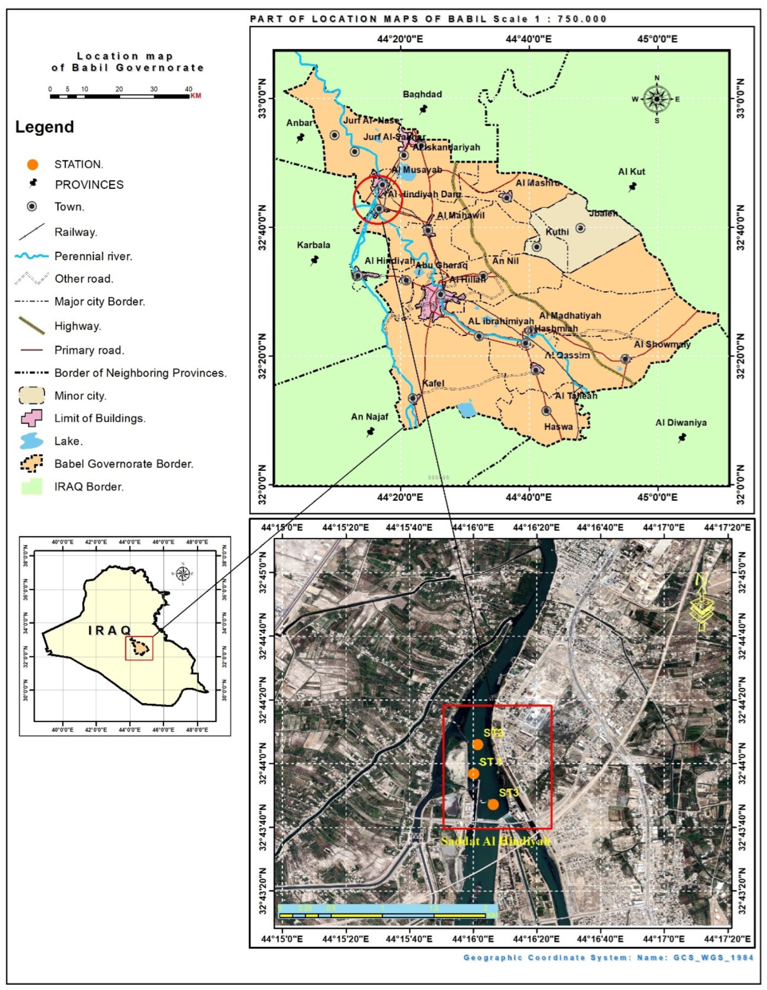
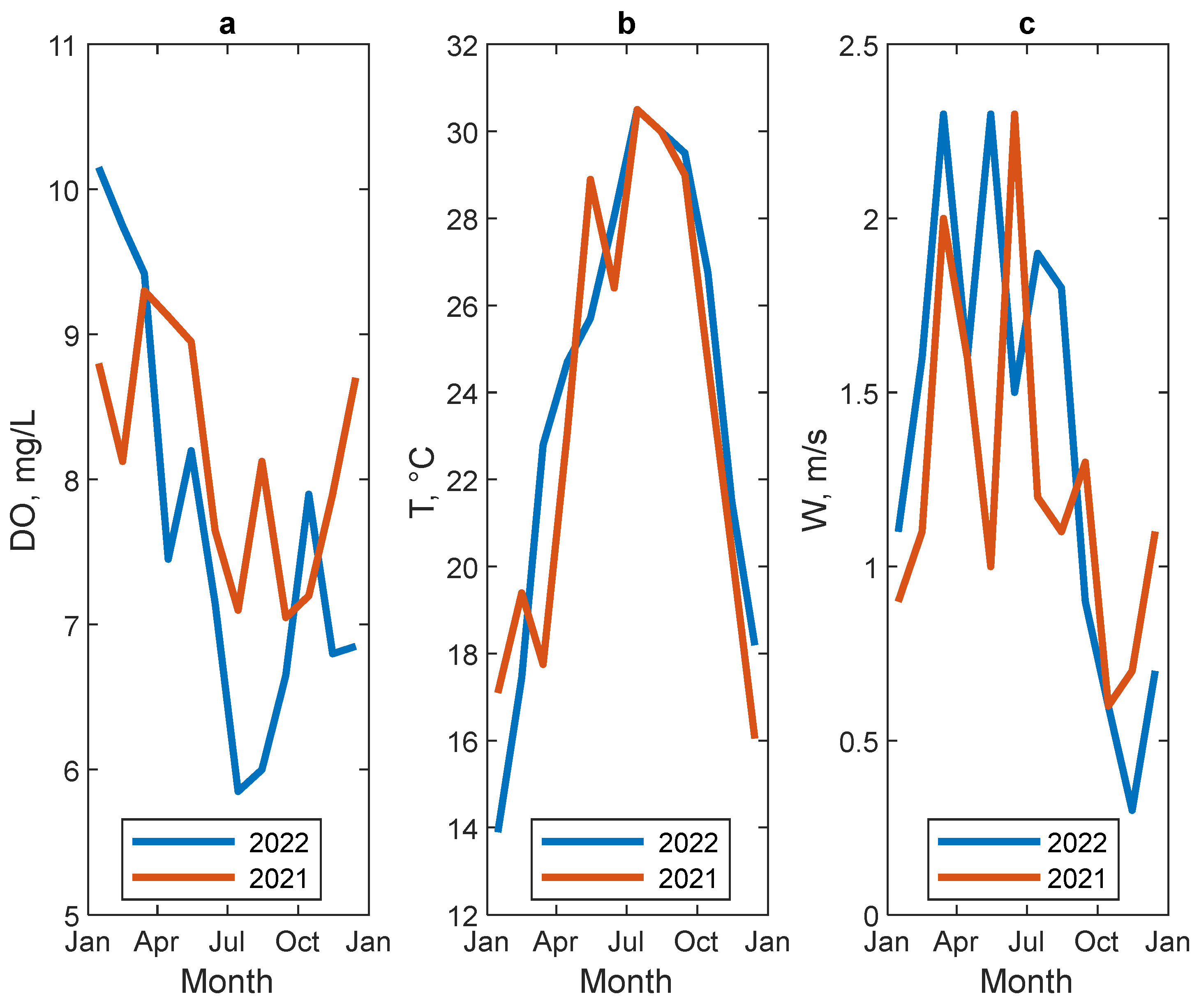
2.2. Study Area and Field Data

Saddat Al-Hindiyah is a reservoir located in the Babylon Governorate, Iraq, on the Euphrates River (Figure 2). It is 31.4 m above sea level and situated between latitude 32°43′55.5′′ N and longitude 44°16′05.7′′ E. It is thought to be the oldest and most significant irrigation project in Iraq. The reservoir serves as the main source of water for the Hilla River and is regarded as its headwater. Along with the reservoir inflows, a significant amount of sediments and floating plants have been observed to be entering the reservoir. The aquatic ecological health of the waterbody is negatively impacted by these constituents in various ways. Therefore, the downstream river watershed ecosystem as well as the reservoir itself may suffer from dissolved oxygen depletion effects brought on by these components. Consequently, there is a necessity to explore the yearly cycle of DO concentrations in the reservoir.

Three sampling locations (ST1, ST2, and ST3), as shown in Figure 3, were utilized to collect the datasets used in this study, dissolved oxygen (DO) and water temperature (T), during the study period of two years (2021 and 2022). The entire study area is covered by these locations. The ST1 station is near the dam location, the ST2 station is at the middle of the reservoir, and the ST3 is near the inflow location. During the study period, three samples were taken monthly at each sampling location as a part of the collection process. Throughout the study period, the average monthly water temperature and dissolved oxygen concentrations are displayed in Figure 3 in addition to the wind speed measurements that were taken by the General Authority for Meteorology and Seismic Monitoring—Iraq. It is obvious that both of the water quality parameters (DO and T) have an inverse relationship. Temperature dropped from 30.5 to 13.9 °C in 2022 and from 30.5 to 16.057 °C in 2021, and the DO concentration became higher from 5.85 to 10.15 mg/L in 2022 and from 7.05 to 11.3 mg/L in 2021. Also, the wind speed ranged from 0.3 to 2.3 m/s in 2022 and from 0.6 to 2.3 m/s in 2021.

2.3. Development of the Numerical Model

The numerical model used to simulate the temporal variation of DO in the headwater was developed based on the one-dimensional transport equation of DO in surface waterbodies, which is governed by the general one-dimensional advection diffusion equation. After neglecting the advection and diffusion terms, keeping the reaeration process at the water surface as the only source–sink for DO, and assuming a well-mixed waterbody, the simplified governing equation is as follows [1,19,20]:

$${\displaystyle \frac{\mathrm{d}\mathrm{D}\mathrm{O}}{\mathrm{d}\mathrm{t}}}=\mathrm{S}$$

(13)

where DO is the waterbody dissolved oxygen concentration at any time (mg/L), t is time (s), and S is the dissolved oxygen source–sink term at any time (mg/L/s).

The oxygen reaeration mechanism operates the oxygen mass transport (magnitude and direction) depending on the DO saturation and the actual value in the water as follows [1]:

$$\mathrm{S}=\mathrm{K}\mathrm{a}{(\mathrm{D}\mathrm{O}}_{\mathrm{s}}-\mathrm{D}\mathrm{O})$$

(14)

where Ka is the dissolved oxygen reaeration coefficient at any temperature (T) and can be related to 20 °C by using the Arrhenius equation, Ka_(T) = Ka_{(20 °C)} (1.024)^T−20, and ${\mathrm{D}\mathrm{O}}_{\mathrm{s}}$ is the saturated dissolved oxygen concentration (mg/L) at any temperature (T) and can be determined from the following formulation [14]:

$${\mathrm{D}\mathrm{O}}_{\mathrm{s}}=\mathrm{A}·{\mathrm{e}}^{\left[7.7117 - 1.31403\ln \left(\mathrm{T} + 45·93\right)\right]}$$

(15)

$$\mathrm{A}=\mathrm{B}{\left[1-{\displaystyle \frac{\mathrm{h}}{44.3}}\right]}^{5.25}$$

(16)

where A is a correction factor, h is the elevation of the waterbody above sea level (km), and B is a calibration factor used to calibrate the DO model if necessary.

The reaeration coefficient (Ka) in Equation (14) can be calculated based on the wind speed and water depth as shown in Table 1, where several Ka empirical equations were conducted to predict the reaeration coefficient based on the wind speed measurements at 10 m height above the water surface. The Ka empirical equations in Table 1 requires wind speed to be at a height of 10 m above the water surface; therefore, the local wind speed was transformed to 10 m height as follows [21]:

$${\mathrm{W}}_{\mathrm{Z}}=\left(\ln {\displaystyle \frac{\mathrm{Z}}{{\mathrm{Z}}_0}}-\ln {\displaystyle \frac{{\mathrm{Z}}_1}{{\mathrm{Z}}_0}}\right){\mathrm{W}}_{\mathrm{Z}1}$$

(17)

where W_Z is the desired wind speed (m/s) at elevation Z (m), W_Z1 is the local wind speed (m/s) at elevation Z₁ (m), and Z₀ is the wind roughness height (m).

Finally, to select the best choice for the appropriate Ka values that verifies the validity of the DO model, the statistical errors (MAE and RMSE) were calculated to measure and evaluate the performance of the model based on number of comparisons (N) by comparing the numerical predictions (${\mathrm{D}\mathrm{O}}_{\mathrm{m}\mathrm{o}\mathrm{d}\mathrm{e}\mathrm{l}}$) to the field data (${\mathrm{D}\mathrm{O}}_{\mathrm{d}\mathrm{a}\mathrm{t}\mathrm{a}}$) [22,23,24,25,26].

$$\mathrm{M}\mathrm{A}\mathrm{E}={\displaystyle \frac{\sum _1^{\mathrm{N}}\left|{\mathrm{D}\mathrm{O}}_{\mathrm{m}\mathrm{o}\mathrm{d}\mathrm{e}\mathrm{l}}-{\mathrm{D}\mathrm{O}}_{\mathrm{d}\mathrm{a}\mathrm{t}\mathrm{a}}\right|}{\mathrm{N}}}$$

(18)

$$\mathrm{R}\mathrm{M}\mathrm{S}\mathrm{E}=\sqrt{{\displaystyle \frac{\sum _1^{\mathrm{N}}{\left({\mathrm{D}\mathrm{O}}_{\mathrm{m}\mathrm{o}\mathrm{d}\mathrm{e}\mathrm{l}}-{\mathrm{D}\mathrm{O}}_{\mathrm{d}\mathrm{a}\mathrm{t}\mathrm{a}}\right)}^2}{\mathrm{N}}}}$$

(19)

3. Results and Discussion

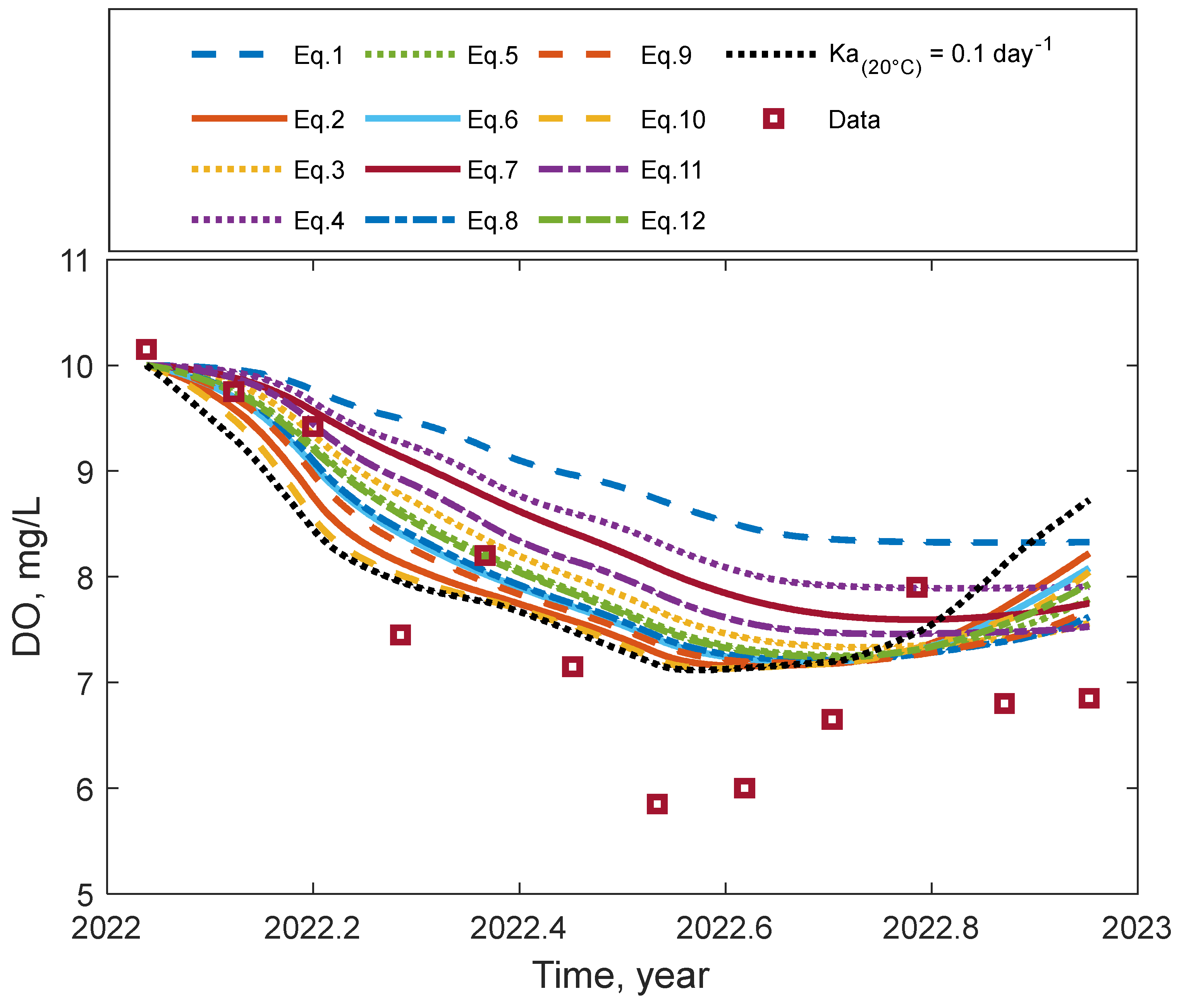
3.1. DO and Ka Numerical Determinations

The developed numerical model was run in the MATLAB environment [version R2021b (9.11), 64-bit (win64)] to simulate the reservoir DO concentrations distribution during the study years. In this model, the numerical solution of Equation (13) was performed based on the dataset in Figure 3, using a suitable time step (0.01 day) and choosing an appropriate Ka_{(20 °C)} value. Since the reaeration process was assumed to be the only DO source–sink in the reservoir, choosing the Ka_{(20 °C)} value forces the DO concentrations to vary significantly. Therefore, different Ka_{(20 °C)} values were explored during the model calibration and validation process. The modeling results showed that the best matching between the model predictions of DO and field data was achieved when the Ka_{(20 °C)} value is 0.1 day⁻¹ in 2021 and 2022 with (MAE: 0.4987 mg/L and RMSE: 0.6390 mg/L) and (MAE: 0.7880 mg/L and RMSE: 0.9344 mg/L), respectively, as depicted in Figure 4 and Figure 5 (see the black dotted curve in both figures for the robust simulation results).

In order to highlight the appropriate Ka empirical equation that simulates the DO concentrations in the reservoir efficiently, the model was calibrated by internally calculating the Ka values using the empirical equations in Table 1. As shown in Figure 4 and Figure 5, different simulation results were generated by each equation with different behaviors, reflecting how Ka equation selecting can impact the numerical determination of DO in surface waterbodies. Accordingly, it was found that Equation (10) (Broecker et al., 1978) followed by Equation (2) (Smith, 1978) gave the best DO simulation results compared to its robust numerical predictions (the black dotted curve in Figure 4 and Figure 5), and then the DO simulation curves generated by the other equations started to become higher further, leading to non-realistic predictions for the reservoir DO concentrations distribution.

Table 2. Statistical errors of DO predictions by using different Ka empirical equations compared to the model prediction of Equation (13) (Ka_{(20 °C)} = 0.1 day⁻¹) in 2021 and 2022.

Ka Equation	2021		2022
	RMSE (mg/L)	MAE (mg/L)	RMSE (mg/L)	MAE (mg/L)
Equation (1)	0.7897	0.6455	1.1773	1.0680
Equation (2)	0.2275	0.1686	0.2209	0.1744
Equation (3)	0.5103	0.4084	0.5868	0.5134
Equation (4)	0.6991	0.5762	0.9183	0.8358
Equation (5)	0.4164	0.3272	0.4866	0.4195
Equation (6)	0.3195	0.2469	0.3492	0.2962
Equation (7)	0.5841	0.4808	0.7938	0.7156
Equation (8)	0.4217	0.3202	0.4477	0.3649
Equation (9)	0.3750	0.2769	0.3918	0.3047
Equation (10)	0.2005	0.1347	0.2324	0.1400
Equation (11)	0.5830	0.4771	0.6708	0.5999
Equation (12)	0.3760	0.2956	0.4492	0.3875

states the statistic errors for each Ka equation compared to the robust simulation results of DO.

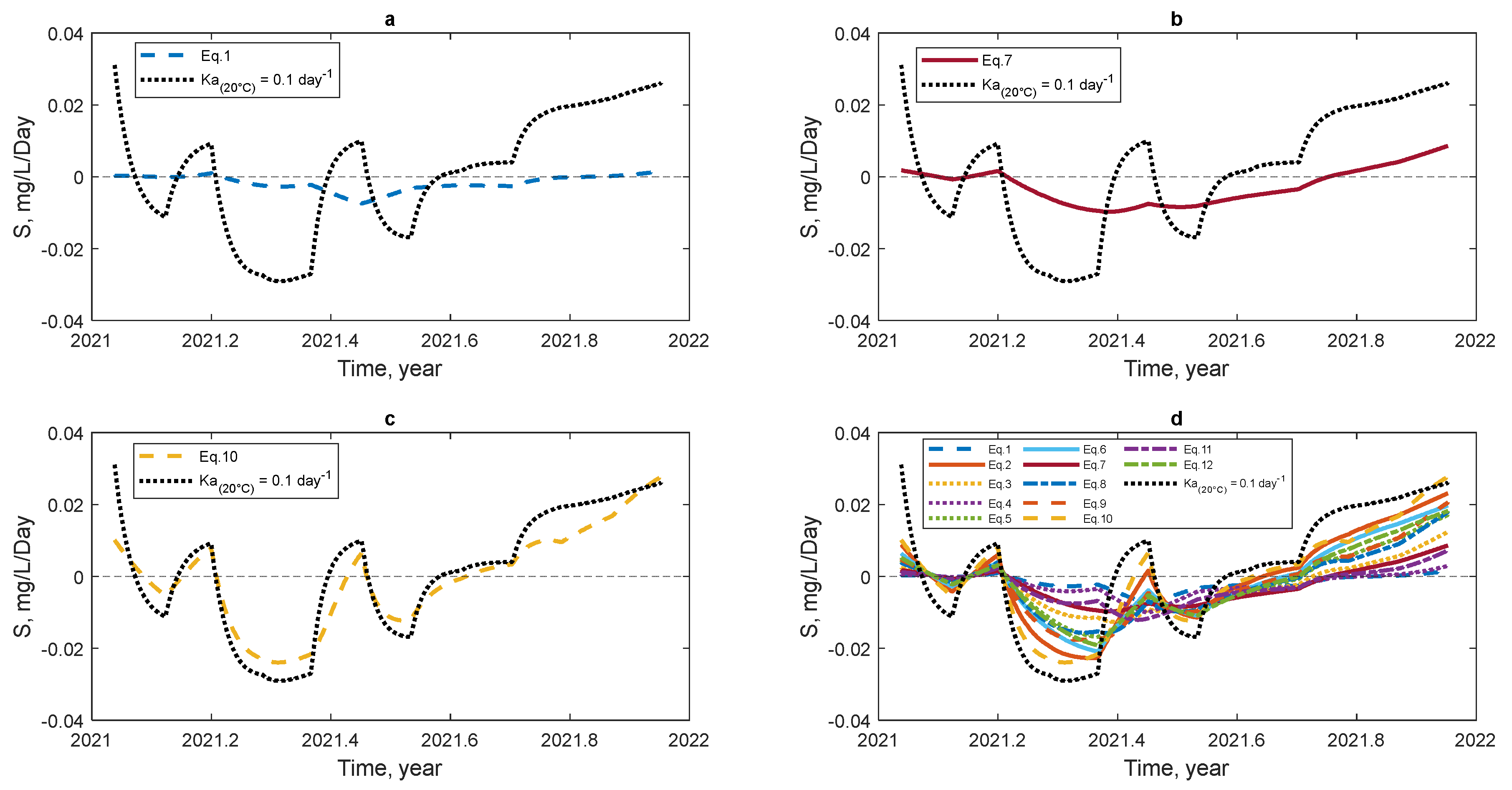
3.2. DO Source–Sink Response to Change Ka Equation

Despite the fact that there are many DO sources–sinks that can produce or consume oxygen in surface waterbodies [27], the present numerical modeling approach predicted the DO yearly cycles efficiently depending on assuming that the reaeration process is the only DO source–sink in the reservoir. However, the Ka equation selection plays a major role in the model predictions robustness due to the influence of Ka values on the oxygen transport mechanisms at the air–water interface of the reservoir waterbody [28]. To reveal the impact of using any selected Ka equation on the DO source–sink amount, the oxygen mass transfer rate per unit volume (Equation (14)) was simulated by using the Ka equations in Table 1 and compared to the robust model predictions.

Figure 6 and Figure 7 show the DO source–sink during 2021 and 2022, respectively, in which positive S values represent the dissolved oxygen source, and negative S values represent the oxygen sink. As depicted, the Ka equation impacts the amount of oxygen transported into or outside the reservoir waterbody significantly. Depending on the dissolved oxygen saturation state, oxygen moves outside the waterbody during the summer season and toward the waterbody during the cold periods especially in winter [29,30]. It is clear that Equation (10) followed by Equation (2) gave more robust predictions compared to the other equations. Nevertheless, the DO source–sink simulation results of Figure 6 and Figure 7 confirm the DO concentrations simulation results of Figure 4 and Figure 5, respectively. Consequently, selecting the unsuitable Ka equation produces or consumes different amounts of oxygen in the waterbody, lowering the model predictions quality.

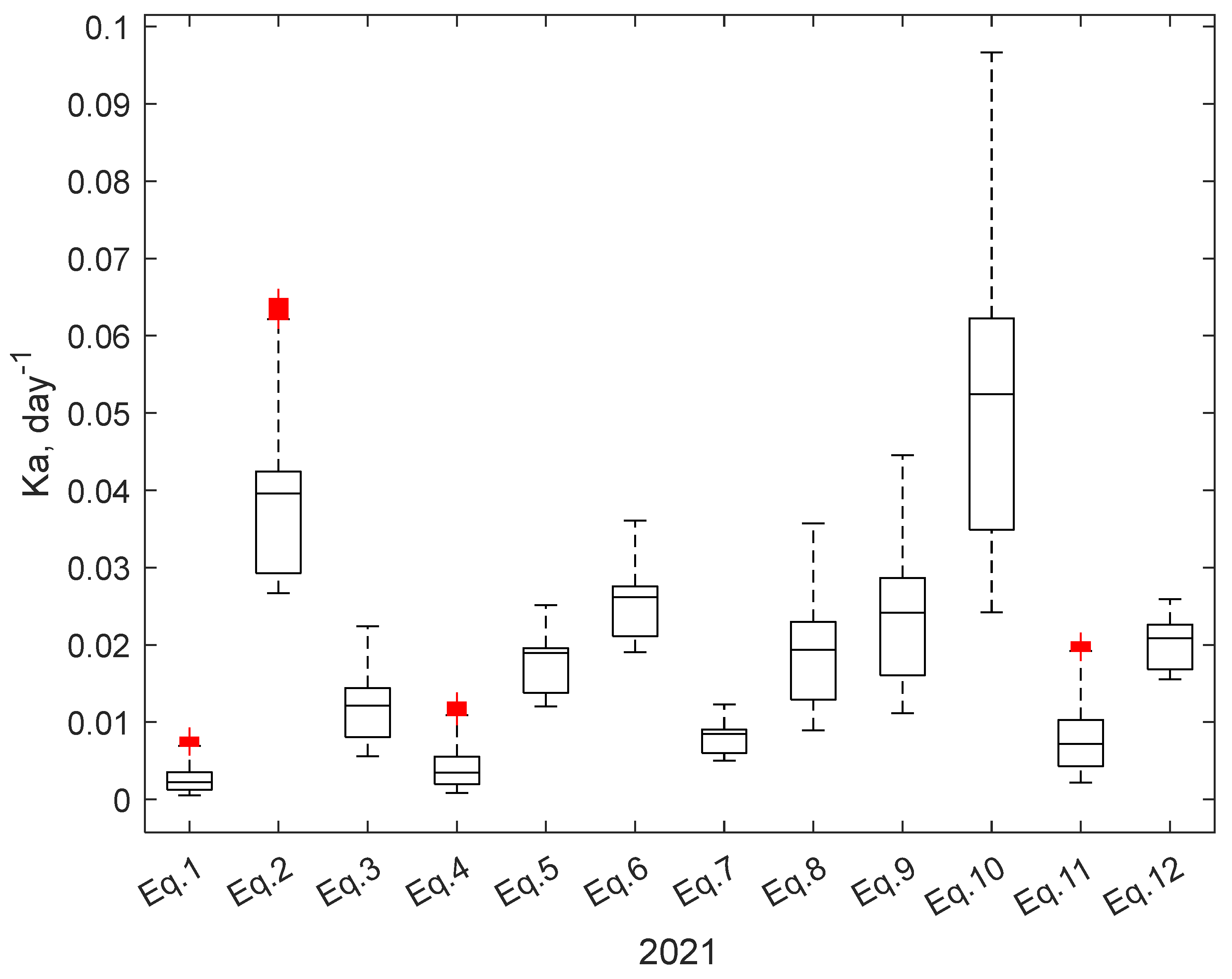
3.3. The Temporal Variation of Reaeration Coefficient

Because water temperature is a direct driving parameter that forces the reaeration coefficient to vary temporally in addition to the vertical mixing by wind, the dissolved oxygen amount is directly influenced by reservoir water temperature [31,32,33]. Hence, wind speed has low variability surrounding the reservoir location (Figure 4, Figure 5, Figure 6 and Figure 7). As a result, the highest DO values were during low temperature conditions and the lowest values were during the high temperature conditions during the summer season. The temporal variation of the Ka value during the simulation years was determined by using all Ka equations and compared to the model predictions of Equation (13) (Ka_{(20 °C)} = 0.1 day⁻¹) as shown in Figure 8 and Figure 9. Emphasizing the main findings of Figure 4, Figure 5, Figure 6 and Figure 7, the highest reaeration rates in the reservoir were during the high temperature conditions, while the lowest rates were during the cold weather conditions. Using Ka equations in addition to the model predictions simulated the Ka values with similar trend, but the outputs were different significantly (Figure 10 and Figure 11). Based on the graphical summary in Figure 10 and Figure 11, the maximum Ka value among all equations ranged between 0.0079 and 0.0951 day⁻¹, and the minimum values ranged between 0.00012 and 0.0231 day⁻¹ in 2022. The maximum Ka value among all equations ranged between 0.0080 and 0.0967 day⁻¹, and the minimum values ranged between 0.00052 to 0.0267 day⁻¹ in 2021.

Accordingly, several Ka equations predicted low reaeration coefficients greatly, while a few equations can simulate the entire study periods well. Comparing the numerical predictions of Ka empirical equations to Equation (13)’s model (Ka_{(20 °C)} = 0.1 day⁻¹) showed that the best robust predictions were Equation (10) followed by Equation (2) compared to the other equations. It is necessary to mention that there is good ordered agreement among all predictions (DO, DO source–sink, and Ka values) in which Equation (13) (Ka_{(20 °C)} = 0.1 day⁻¹), Equation (10), and Equation (2) simulate these predictions in order with ordered statistical errors as shown in Table 2 and Figure 12, showing the values of statistical errors (MAEs) during the simulation years. It is clear that Equation (2) and (10) have the lowest errors compared to other Ka empirical equations. Generally, MAE and RMSE values ranged from 0.1347 to 0.6455 mg/L and from 0.2005 to 0.7897 mg/L in 2021, respectively, and ranged from 0.1400 to 1.0680 mg/L and from 0.2209 to1.1773 mg/L in 2022, respectively. Thus, the best Ka empirical equations that researchers can implement to simulate water quality at the Hilla River headwater are those developed by Broecker et al. (1978) and by Smith (1978).

4. Conclusions

An integrated numerical-modeling-based technique was developed for selecting the best reaeration coefficient (Ka) empirical equation to be implemented for water quality modeling in rivers, lakes, and reservoirs. The simulation findings highlighted that the correct and accurate selection of the reaeration coefficient values through empirical equations is an important factor affecting the accuracy of the dissolved oxygen predictions (DO). Each equation often yields reaeration coefficients that are different from the others with wide-ranging statistical errors, simulating the water system dissolved oxygen with different accuracies. Using direct field measurements at the Hilla River headwater (Saddat Al-Hindiyah Reservoir, Babylon, Iraq) obtained that the reaeration coefficient empirical equations developed by Broecker et al. (1978) and Smith (1978) are the most appropriate equations for reservoir water quality modeling purposes with a reservoir reaeration coefficient of 0.1 day⁻¹ at 20 °C. For all Ka empirical equations, high water temperature increases the reaeration coefficients, and low temperature values make it lower. In addition, the selection technique requires the yearly cycle of DO, DO source–sink, and Ka numerical predictions to be in well-matched accuracies with less statistical errors for selecting the appropriate Ka empirical equation. Thus, direct field measurements of dissolved oxygen temporal variation lead to accurate reaeration coefficients by using the applicable Ka empirical equation only.

References

1. Chapra, S.C. Surface Water-Quality Modeling; Waveland Press, Inc.: Long Grove, IL, USA, 2008. [Google Scholar]
2. Abouelsaad, O.; Matta, E.; Omar, M.; Hinkelmann, R. Numerical simulation of Dissolved Oxygen as a water quality indicator in artificial lagoons–Case lagoons—Case study El Gouna, Egypt. Reg. Stud. Mar. Sci. 2022, 56, 102697. [Google Scholar] [CrossRef]
3. Ferreira, M.D.S.; Soeira, T.V.R.; Ferreira, D.C.; da Luz, M.S.; Poleto, C.; Gonçalves, J.C.d.S.I. The effect of sds surfactant on surface reaeration coefficient: A laboratory scale approach. Ambient. Agua-Interdiscip. J. Appl. Sci. 2020, 15, 1. [Google Scholar] [CrossRef]
4. Abu Hanipah, A.H.; Guo, Z.R. Reaeration Caused by Intense Boat Traffic. Asian J. Water Environ. Pollut. 2019, 16, 15–24. [Google Scholar] [CrossRef]
5. Hull, V.; Parrella, L.; Falcucci, M. Modelling dissolved oxygen dynamics in coastal lagoons. Ecol. Model. 2008, 211, 468–480. [Google Scholar] [CrossRef]
6. Correa-González, J.C.; Chávez-Parga, M.d.C.; Cortés, J.A.; Pérez-Munguía, R.M. Photosynthesis, respiration and reaeration in a stream with complex dissolved oxygen pattern and temperature dependence. Ecol. Model. 2014, 273, 220–227. [Google Scholar] [CrossRef]
7. Chu, C.R.; Jirka, G.H. Wind and Stream Flow Induced Reaeration. J. Environ. Eng. 2003, 129, 1129–1136. [Google Scholar] [CrossRef]
8. de Souza Inácio Gonçalves, J.C.; Silveira, A.; Lopes Júnior, G.B.; da Luz, M.S.; Simões, A.L.A. Reaeration Coefficient Estimate: New Parameter for Predictive Equations. Water Air Soil Pollut. 2017, 228, 307. [Google Scholar] [CrossRef]
9. Ota, R.O.; Egbe, J.G. Comparative Empirical Analysis for Determination of Re-Aeration Rate Constant of Otamiri and Kaduna Rivers. Int. J. Water Resour. 2024, 6, 168. [Google Scholar]
10. Klaus, M.; Vachon, D. Challenges of predicting gas transfer velocity from wind measurements over global lakes. Aquat. Sci. 2020, 82, 1–17. [Google Scholar] [CrossRef]
11. Cole, J.; Bade, D.L.; Bastviken, D.; Pace, M.L.; Van de Bogert, M. Multiple approaches to estimating air-water gas exchange in small lakes. Limnol. Oceanogr. Methods 2010, 8, 285–293. [Google Scholar] [CrossRef]
12. Gelda, R.K.; Auer, M.T.; Effler, S.W.; Chapra, S.C.; Storey, M.L. Determination of Reaeration Coefficients: Whole Lake Approach. J. Environ. Eng. 1996, 122, 269–275. [Google Scholar] [CrossRef]
13. Benson, A.; Zane, M.; Becker, T.E.; Visser, A.; Uriostegui, S.H.; DeRubeis, E.; Moran, J.E.; Esser, B.K.; Clark, J.F. Quantifying reaeration rates in alpine streams using deliberate gas tracer experiments. Water 2014, 6, 1013–1027. [Google Scholar] [CrossRef]
14. Cole, T.M.; Wells, S.A. CE-QUAL-W2: A Two-Dimensional, Laterally Averaged, Hydrodynamic and Water Quality Model, 2006; Version 3.5. Available online: https://pdxscholar.library.pdx.edu/cengin_fac (accessed on 18 June 2024).
15. Antonopoulos, V.Z.; Gianniou, S.K. Simulation of water temperature and dissolved oxygen distribution in Lake Vegoritis, Greece. Ecol. Model. 2003, 160, 39–53. [Google Scholar] [CrossRef]
16. Fang, X.; Stefan, H.G. Interaction between Oxygen Transfer Mechanisms in Lake Models. J. Environ. Eng. 1995, 121, 447–454. [Google Scholar] [CrossRef]
17. Gualtieri, C. Verification of wind-driven volatilization models. Environ. Fluid Mech. 2006, 6, 1–24. [Google Scholar] [CrossRef]
18. Al-Zubaidi, H.A.; Wells, S.A. 3D numerical temperature model development and calibration for lakes and reservoirs: A case study. In Proceedings of the World Environmental and Water Resource Congress, Sacramento, CA, USA, 18 May 2017; pp. 595–610. [Google Scholar] [CrossRef]
19. Mowjood, M.I.M.; Kasubuchi, T. Effect of convection on the exchange coefficient of oxygen and estimation of net production rate of oxygen in ponded water of a paddy field. Soil Sci. Plant Nutr. 2002, 48, 673–678. [Google Scholar] [CrossRef]
20. Al-Zubaidi, H.A.; Naje, A.S.; Al-Ridah, Z.A.; Chelliapan, S.; Sopian, K. Numerical Modeling of Reaeration Coefficient for Lakes: A Case Study of Sawa Lake, Iraq. Ecol. Eng. Environ. Technol. 2024, 25, 145–153. [Google Scholar] [CrossRef]
21. Ro, K.S.; Hunt, P.G. New Unified Equation for Wind-Driven Surficial Oxygen Transfer into Stationary Water Bodies. Trans. ASABE 2006, 49, 1615–1622. [Google Scholar] [CrossRef]
22. Robeson, S.M.; Willmott, C.J. Decomposition of the mean absolute error (MAE) into systematic and unsystematic components. PLoS ONE 2023, 18, e0279774. [Google Scholar] [CrossRef]
23. Chai, T.; Draxler, R.R. Root mean square error (RMSE) or mean absolute error (MAE)?—Arguments against avoiding RMSE in the literature. Geosci. Model Dev. 2014, 7, 1247–1250. [Google Scholar] [CrossRef]
24. Mugume, I.; Basalirwa, C.; Waiswa, D.; Reuder, J.; Mesquita, M.D.S.; Tao, S.; Ngailo, T.J. Comparison of Parametric and Nonparametric Methods for Analyzing the Bias of a Numerical Model. Model. Simul. Eng. 2016, 2016, 7530759. [Google Scholar] [CrossRef]
25. Wang, W.; Lu, Y. Analysis of the Mean Absolute Error (MAE) and the Root Mean Square Error (RMSE) in Assessing Rounding Model. IOP Conf. Ser. Mater. Sci. Eng. 2018, 324, 012049. [Google Scholar] [CrossRef]
26. Al-Dalimy, S.Z.; Al-Zubaidi, H.A.M. Application of QUAL2K Model for Simulating Water Quality in Hilla River, Iraq. J. Ecol. Eng. 2023, 24, 272–280. [Google Scholar] [CrossRef]
27. Bengtsson, L.; Ali-Maher, O. The dependence of the consumption of dissolved oxygen on lake morphology in ice covered lakes. Hydrol. Res. 2020, 51, 381–391. [Google Scholar] [CrossRef]
28. Zhang, F.; Shi, X.; Zhao, S.; Arvola, L.; Huotari, J.; Hao, R. Equilibrium simulation and driving factors of dissolved oxygen in a shallow eutrophic Inner Mongolian lake (UL) during open-water period. Water Supply 2022, 22, 6013–6031. [Google Scholar] [CrossRef]
29. Chukwuma, A.N.; Ugbebor, J.; Ugwoha, E. Modeling of re-aeration coefficient For Nkisa River, Egbema, Rivers State, Nigeria. Water Pract. Technol. 2024, 19, 200–212. [Google Scholar] [CrossRef]
30. Palshin, N.; Zdorovennova, G.; Efremova, T.; Bogdanov, S.; Terzhevik, A.; Zdorovennov, R. Dissolved oxygen stratification in a small lake depending on water temperature and density and wind impact. IOP Conf. Ser. Earth Environ. Sci. 2021, 937, 032019. [Google Scholar] [CrossRef]
31. Hill, N.B.; Riha, S.J.; Walter, M.T. Temperature dependence of daily respiration and reaeration rates during baseflow conditions in a northeastern U.S. stream. J. Hydrol. Reg. Stud. 2018, 19, 250–264. [Google Scholar] [CrossRef]
32. Al-Zubaidi, H.A.M.; Wells, S.A. Comparison of a 2D and 3D Hydrodynamic and Water Quality Model for Lake Systems. In Proceedings of the World Environmental and Water Resources Congress 2018: Watershed Management. Irrigation and Drainage, and Water Resources Planning and Management, Minneapolis, MN, USA, 31 May 2018; pp. 74–84. [Google Scholar] [CrossRef]
33. Demars, B.O.L.; Manson, J.R. Temperature dependence of stream aeration coefficients and the effect of water turbulence: A critical review. Water Res. 2013, 47, 1–15. [Google Scholar] [CrossRef]
Figure 1. Conceptual framework of the study.
Limnolrev 25 00015 g001
Figure 2. Study area and sampling stations.
Limnolrev 25 00015 g002
Figure 3. Monthly averaged field measurements of (a) dissolved oxygen (DO), (b) water temperature (T), and (c) wind speed (W) during 2021 and 2022.
Limnolrev 25 00015 g003
Figure 4. The dissolved oxygen (DO) numerical simulation for the Hilla River headwater using different Ka empirical equations in addition to the model predictions of Equation (13) (Ka(20 °C) = 0.1 day−1) compared to field data during 2021.
Limnolrev 25 00015 g004
Figure 5. The dissolved oxygen (DO) numerical simulation for the Hilla River headwater using different Ka empirical equations in addition to the model predictions of Equation (13) (Ka(20 °C) = 0.1 day−1) compared to field data during 2022.
Limnolrev 25 00015 g005
Figure 6. The dissolved oxygen (DO) source–sink numerical simulation for the Hilla River headwater using different Ka empirical equations (ad) in addition to the model predictions of Equation (13) (Ka(20 °C) = 0.1 day−1) compared to field data during 2021.
Limnolrev 25 00015 g006
Figure 7. The dissolved oxygen (DO) source–sink numerical simulation for the Hilla River headwater using different Ka empirical equations (ad) in addition to the model predictions of Equation (13) (Ka(20 °C) = 0.1 day−1) compared to field data during 2022.
Limnolrev 25 00015 g007
Figure 8. The reaeration coefficients (Ka) numerical simulation for the Hilla River headwater using different empirical equations compared to the model prediction of Equation (13) (Ka(20 °C) = 0.1 day−1) during 2021.
Limnolrev 25 00015 g008
Figure 9. The reaeration coefficients (Ka) numerical simulation for the Hilla River headwater using different empirical equations compared to the model prediction of Equation (13) (Ka(20 °C) = 0.1 day−1) during 2022.
Limnolrev 25 00015 g009
Figure 10. Graphical summarization for the Hilla River headwater reaeration coefficients (Ka) using different empirical equations during 2021.
Limnolrev 25 00015 g010
Figure 11. Graphical summarization for the Hilla River headwater reaeration coefficients (Ka) using different empirical equations during 2022.
Limnolrev 25 00015 g011
Figure 12. MAEs of DO predictions by using different Ka empirical equations in 2021 and 2022.
Limnolrev 25 00015 g012