
A Distributed Algorithm for the Assignment of the Laplacian Spectrum for Path Graphs

Department of Engineering for Innovation, University of Salento, via per Monteroni, 73100 Lecce, Italy
Mathematics 2023, 11(10), 2359; https://doi.org/10.3390/math11102359
Submission received: 28 March 2023
/
Revised: 16 May 2023
/
Accepted: 17 May 2023
/
Published: 18 May 2023
(This article belongs to the Special Issue Applications of Algebraic Graph Theory and Its Related Topics)
Abstract
:In this paper, we bring forward a distributed algorithm for the assignment of a prescribed Laplacian spectrum for path graphs by means of asymmetric weight assignment. We first describe the meaningfulness and the relevance of this mathematical setting in modern technological applications, and some examples are reported, revealing its practical usefulness in a variety of applications. Then, the solution is derived both theoretically and through an algorithm. Special attention is devoted to a distributed implementation of the main algorithm, which is a valuable feature for several modern applications. Finally, the positivity is discussed, which is revealed to be a consequence of the strict interlacing property.
MSC:
93B55; 05C50; 94C15; 39A06; 37N35; 37M101. Introduction
In recent decades, an increasing number of research activities arose studying the behavior of interacting devices for applications in disparate technological areas, giving rise to the subject of networked systems [1,2,3,4]. Network topology became a fundamental new design paradigm, and mainly the spectral properties of some graph-related matrices, such as adjacency or Laplacian matrix, were researched.
The Laplacian matrix of a graph is a potent tool for the theoretical study and design of many contemporary technological applications where the graph encodes local interactions among agents, thus including [5,6] multi-agent systems, computer networks, sparse coding, and collaborative robotic networks. In such applications, the spectral properties of a graph-related matrix, and especially the Laplacian matrix, often play a key role in explaining some internal structure or condition, such as clustering, partitioning, consensus or synchronization [5,7,8]. Grounded Laplacian refers to the main submatrix that results from eliminating the i-th row and column of a Laplacian matrix. The performance of various applications is also directly correlated with the spectral features of a grounded Laplacian, which have undergone many studies in recent years as well [9,10]. In this paper, we shed a light on the class of Laplacian matrices associated with path graphs, which have the structure of (asymmetric) Jacobi matrices, and they constitute a class of graphs of great importance which has been widely studied over the years [11,12,13].
On the one hand, from a mathematical standpoint, this topic comes within the category of inverse eigenvalue problems, that is, the existence analysis and computation of structured matrices with assigned eigenstructure [14], which has a long history among mathematicians and it is still widely debated [15,16,17]. With reference to such literature, the contribution of this paper is the derivation of an algorithm, which can be distributed with respect to the nodes of the path, and this is a fundamental peculiarity for several modern applications, as detailed in Section 2.
On the other hand, however, the topic of the present paper stems from modern applications, and this makes the challenge different from the classical mathematical settings, as described in [14]. It also has strong connections with control systems theory, and more specifically, it is close to the pole allocation through feedback [18,19,20]. As a final remark, it is worth noting that the knowledge of the Laplacian spectrum allows to monitor the system evolution and detect any anomaly caused by edge malfunctioning or malicious behaviors [21,22].
An early short version of this work was presented in [23]. The paper is organized as follows. In Section 2, after a brief introduction of the notation, we provide some motivating examples that are strongly related to the mathematical problem. In Section 3, the main results of the paper are derived; first, a global algorithm solving the stated problem is deduced using and inductive logic over n, then, it is rearranged to implement it in a distributed fashion, where each node can compute its own weights based only on data gathered by its neighborhood. Here, the analysis is thorough, including complete proofs for all statements. Finally, a discussion on the positivity of the gains provided by the algorithm closes the paper. Furthermore, this paper contains a much improved comprehensive and thorough treatment. A final section describes an illustrative example in the distributed setting for a network of six nodes.
Notation
We now briefly introduce the notation adopted in this paper and we report some basic facts of Graph Theory that are useful to understand the following sections. Given , denotes its -th entry and its i-th column, while is the submatrix obtained by removing the i-th row and j-th column of A. The Laplace expansion rule for the computation of the determinant of a square matrix is: .
A nonnegative (positive) matrix is a matrix with the property (). A matrix is combinatorially symmetric [24] or structurally symmetric when it holds that if and only if . A matrix is called generalized row stochastic matrix if there exists a so that for any and zero row sum matrix if such a c is . In this paper, we deal with zero-row sum combinatorially symmetric matrices [25]. In the following, we denote by the spectrum of a matrix , namely the set of its eigenvalues, and by the spectral radius of A, i.e., the maximum modulus of its eigenvalues. For a reference book on polynomials, the reader is referred to the book [26].
A graph is a mathematical object made of a vertex set and an edge set. A path connecting vertex with is a subset of edges . Given a graph , we define the adjacency matrix as if and if , and the weighted adjacency matrix as with if and if . Finally, the weighted Laplacian matrix is defined as if and . By construction, for any , i.e., the Laplacian is a zero-row sum matrix. Finally, the matrix obtained by removing the ℓ-th row and column of is the so-called grounded Laplacian matrix (or Dirichlet Laplacian matrix) (see for information [9,27]), which we denote in the following by .
Conversely, for a graph , we use the symbol to denote the set of all possible weighted Laplacian matrices whose graph is ; in other words, denotes the set of all zero-row sum -structured square matrices.
2. Motivating Examples
In this section, we provide an abstract multi-agent system setting where the problem afforded in this paper is meaningful, and then, we provide some examples of several modern technological fields where the algorithms provided in this paper can be effectively adopted.
2.1. Collaborative Multi-Agent Systems and Consensus Networks
In the following, we describe the abstract multi-agent setting [5,28], which is the mathematical framework of the applications described soon after. Given a set of N variables , updating as , where is an update variable chosen by each node i. A graph describes the communication among nodes, namely two neighbor nodes i, j which are connected through an edge are able to exchange their values (that is, node i sends to node j and vice versa), so node i can choose , where are set by node i. The resulting dynamics of the team can be compactly written using a vector built as for a , which belongs to the set , and the evolution of the network is governed by the spectrum of [29]. In this framework, the design of asymmetric gains was recently studied [30,31,32] to increase the convergence rate, which is a key feature; this was recently explored in [33,34,35].
Assume now that one node, e.g., node 1, takes the role of a leader and it adds a driving signal to its update variable, namely:
to take control of the team evolution [36]. This setting is known as leader follower network, [37,38,39] and its dynamics is described by:
with or, equivalently, using the transfer function:
where and , and hence, the zeros of and are the poles and zeros of system (2), (3), so that their allocation allows to set all the fundamental input-output properties of the team (such as the zero-pole distance and, in turn, to influence several dynamical properties of the team driven by a prescribed node, such as controllability and observability of the whole network from node 1). It is worth remarking that coprimeness between and is necessary for the full control of the team by the leader [40].
2.2. Some Examples of Applications Scenarios
The above setting is applied to several technological modern applications, for example: (a) Robotic networks. In this application area, the above setting is widely used to perform global actions (such as rendez-vous, deployment, formation control) without recurring to a supervisory device [41]. (b) Wireless sensor networks. Several fundamental issues of wireless sensor networks are solved using the above setting, for example the synchronization problem [42,43] and the average value of a measured environmental quantity [44]. (c) Vehicle platooning. The above setting is adopted to model the dynamics of vehicles platoon, where Laplacian and grounded Laplacian of path graphs are well suited to describe the common case of bidirectional non-cyclic interactions between the agents [45]. It is worth remarking that weight asymmetry has already been investigated [46] to improve the team performances. (d) Electrical power systems. The multi-agent setting is widely adopted when the numerous challenges of the evolution of the electric grid toward a smart grid are taken into account [47,48,49].
2.3. Problem Statement
Based on the motivating examples introduced so far, we introduce the Problem Statement afforded in the following.
Problem 1.
Consider a graph , and two polynomials , having zeros as satisfying , compute gains , such that if and if satisfying and .
Remark 1.
The above Problem Statement is strictly related to the examples in Section 2.2, and does not include the possibility of overlap between Λ and , which is an unfavorable condition in most applications (as, for example, it implies the loss of controllability and observability by the leader [50]).
3. Problem Solution
The proposed solution follows an inductive approach over . We start with the solution of and , then we extend the solution to a generic n through an iterative algorithm.
3.1. Preliminary Results on n = 2 and n = 3
Consider , which is described by the following matrices:
For any , the solution of the problem can be parametrized as:
We now consider case when ℓ is a leaf, that is:
with associated grounded Laplacian
The computation of the characteristic polynomial shows that:
where
Imposing Equations (7) and (8) for given and allows to compute the weights , , and the two polynomials , . In turn, by making use of the solution (5), it is easy to compute the remaining coefficients , from the polynomials , obtained in the previous step. In the following, we prove that the above procedure can be extended to a general .
3.2. A Recursive General Solution When ℓ Is a Leaf
We are now ready to derive a solution for a generic . It follows an inductive logic over and the solution is recursive.
Theorem 1.
Let be a path graph and node 1 a leaf node, and , be, respectively, its weighted Laplacian and grounded Laplacian. Take two polynomials and such that their zeros satisfy the Problem Statement (Section 2.3).
There always exist such that and , and they can be computed using Algorithm 1.
| Algorithm 1: Computation of the edge weights as the solution of the Problem Statement (Section 2.3). |
Data: , Result: , initialization: , , , for all  |
Proof.
For a path graph, , and
where . Define:
using the Laplace rule for the determinant along the first line, one can further elaborate:
where (respectively, ) is the characteristic polynomial of the Laplacian (respectively, grounded Laplacian) of the path graph made of nodes once that node n is removed.
The above computation shows that the following iterative relations hold:
Let now and be two polynomials having and as zeros, respectively. Forcing and into Equations (11) and (12), one has:
and, exploiting their expanded form, namely and , it is possible to elaborate further (13) as:
and to see that it is possible to have the desired polynomials if the weights , and the coefficients satisfy:
and
Consider now the first two equations. Inserting the second into the first one gives , so that we choose to set:
Consider now the two equations at the second line. Inserting the second relation into the first one has , and considering the previous choice of we obtain and, proceeding iteratively backwards:
Substituting these values into the second column, one obtains:
and, in turn, with the above choices, it is possible to compute:
as functions of the coefficients of and .
The above procedure allows us to compute the edge weights and together with the two polynomials (respectively, ) of the path graph of nodes obtained by removing node n.
Iterating recursively the previous procedure allows computing all coefficients , as follows.
First note that Equations (11) and (12) can be written in a general form for a Path Graph with choosing j as grounded node, namely:
for and , , which extend Equations (11) and (12).
Put the polynomials , computed in the previous step as reference polynomials into the two Equation (19) for . This allows to compute together with and . Iterating this logic using (19) backwards until allows effectively to obtain all , and it can be effectively encapsulated into an algorithm, as Algorithm 1. □
It is worth noting that Algorithm 1 must be iterated a finite number of steps, equal to the eccentricity of the leader node (namely, the length of a longest shortest path starting at the leader node). This makes the proposed algorithm well suited as a preliminary routine to be run before the main application.
4. A Distributed Implementation of Algorithm 1
One key remark for modern engineering and technological applications is that Algorithm 1 is suited to be implemented in a distributed fashion. In such a case, each node can retrieve the weights of its algorithm by processing data received by its neighbor only.
To achieve this goal, the leader should:
- Compute the polynomials and starting from the desired zeros and set them as reference polynomials.
- Compute:to obtain the value of its own weight and the polynomial through the computation of its coefficients:
- Transmit , and to node .
When node n ends the above elaboration, based on the received data, node can trigger its elaboration as follows:
- Retrieve and by performing the following elaboration:
- Then:
- Transmit , and to node .
Based on the above elaboration, node is able compute its own weights and through an elaboration on the received data only. The above steps can be generalized using (19), and hence, it is possible to organize the algorithm so that it can be executed in a distributed fashion, as follows. Consider a node ; upon receipt of , and from node , node ℓ should:
- Retrieve and by performing the following elaboration:
- Then:
- Transmit , and to node .
The above procedure allows each node ℓ to compute its own gains , through an elaboration of local information only (namely, data received from its neighbor). The technical requirement to achieve this is that each node j should be able to send two vectors encoding the coefficients of the two polynomials , .
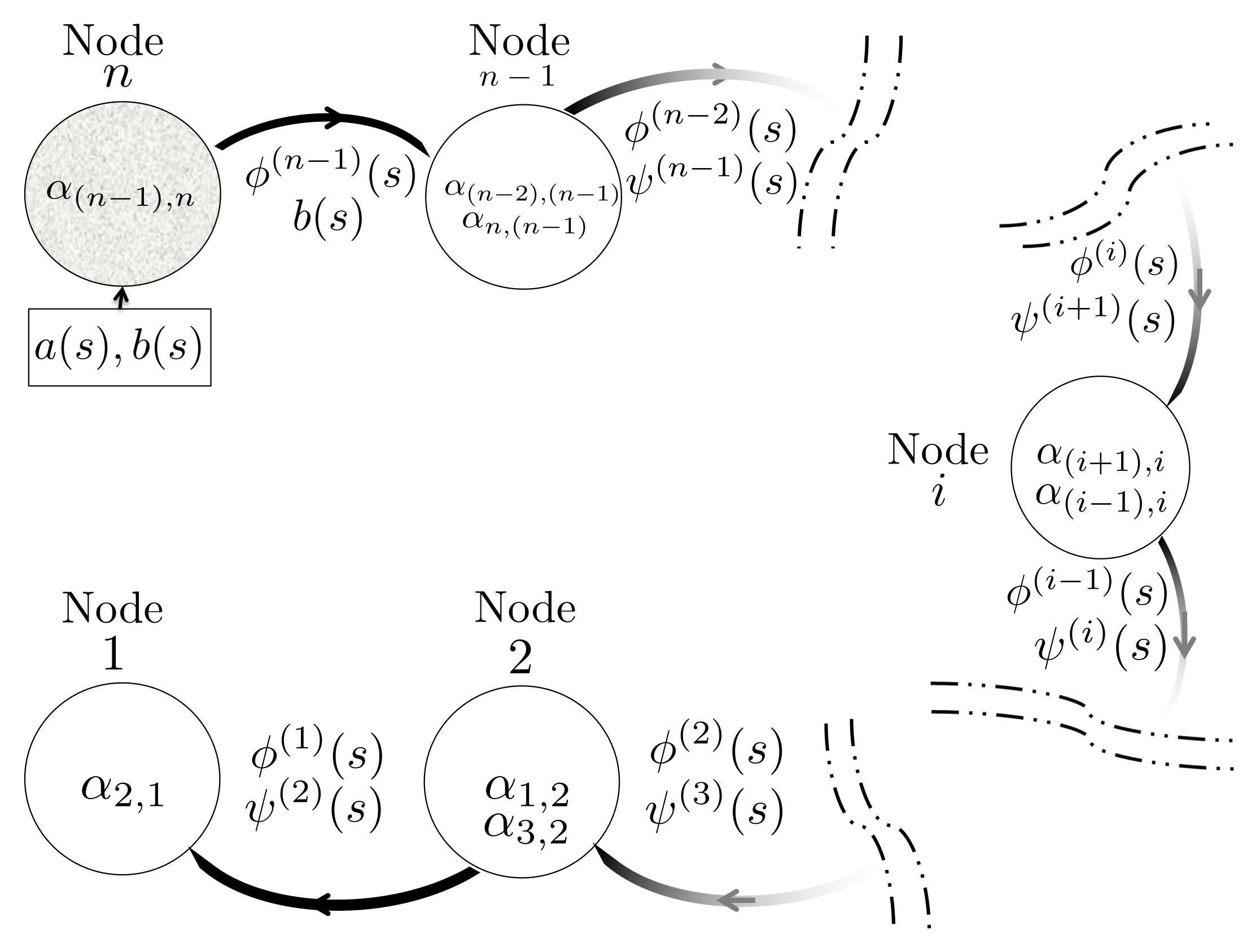
The architecture of the distributed implementation of Algorithm 1 is depicted in Figure 1. Finally, it is worth remarking that the algorithm has finite time execution equal to n time steps so that it can be run as a preliminary routine before other operations in applications.
5. A Final Remark on the Solution of Algorithm 1
In this section, we discuss the sign of the weights obtained as solutions of Algorithm 1, and it is revealed that the condition is a consequence of the relative location of , in the complex plane. In other words, if the interlacing property is set for , beforehand, then the solution of Algorithm 1 always has the property .
Theorem 2.
Let and be two polynomials satisfying the Problem Statement (Section 2.3). Then, Algorithm 1 always provides positive weights satisfying and .
Proof.
Algorithm 1 provides by solving recursively Equation (13), so we prove the statement by showing that, if and satisfy the interlacing property, then the solutions of Equation (13) are positive weights and a pair of polynomials , , which in turn satisfy the interlacing property between themselves. This allows to trigger a recursive logic, which proves that all are positive.
From Equation (13), it is possible to obtain so that and, considering that and analogously for , we obtain , which is positive under the strict interlacing condition between and provided by the Problem Statement. Consider now , which is a monic polynomial of degree . Computing at several points and , one has: because and under (13), and , , and , so that, if denotes the largest zero of , then . If contains any zero of , the computation of and backwards (iterating the above reasonings from to 0) allows to obtain .
Consider now the second of Equation (13), which can be written as and the zeros of , satisfy . For the same reasons as before, . Building the polynomial and defining as the zeros of , it is possible to prove analogously that . □
6. An Illustrative Example
In this section, we provide an illustrative example on the distributed implementation of the Algorithm on a network of six nodes.
Consider that a leaf of a path graph of six nodes starts the algorithm setting and .
According to Section 4, it computes and . Finally, it sends , and .
Once that node 5 receives its data, it computes: , , and then, , . It sends , and to node 4.
The Algorithm prosecutes at node 4 with the values , , and then, , . It sends data to node 3, which computes , , and then, , , and sends data to node 2, which in turn computes , , and then, .
The resulting Laplacian matrix is as follows:
7. Conclusions
This paper proposes an algorithm for the assignment of the Laplacian eigenvalues by a suitable choice of edge gains. An iterative algorithm is derived first, after which a distributed implementation is sought, and its usefulness is also shown using an illustrative example. Several research directions are currently under investigation, which includes more complex kinematics models, such as [51], as well as the analysis of several different graph topologies [1].
Funding
This work was partially supported by the European Union’s Horizon 2020 research and innovation program under the project EUMarineRobots: Marine robotics research infrastructure network, grant agreement N.731103 (call H2020-INFRAIA-2017-1-two-stage).
Data Availability Statement
The datasets generated for this study are available on request to the corresponding author.
Conflicts of Interest
The authors declare that the research was conducted in the absence of any commercial or financial relationships that could be construed as a potential conflict of interest.
References
- Bullo, F. Lectures on Network Systems; Kindle Direct Publishing: Seattle, DC, USA, 2020; Volume 1. [Google Scholar]
- Mullender, S. Distributed Systems; ACM: New York, NY, USA, 1990. [Google Scholar]
- Qu, Z. Cooperative Control of Dynamical Systems: Applications to Autonomous Vehicles; Springer: Berlin/Heidelberg, Germany, 2009; Volume 3. [Google Scholar]
- Yick, J.; Mukherjee, B.; Ghosal, D. Wireless sensor network survey. Comput. Netw. 2008, 52, 2292–2330. [Google Scholar] [CrossRef]
- Bullo, F. Lectures on Network Systems, 1.6 ed.; Kindle Direct Publishing: Seattle, DC, USA, 2022. [Google Scholar]
- Gao, S.; Tsang, I.W.H.; Chia, L.T. Laplacian sparse coding, hypergraph laplacian sparse coding, and applications. IEEE Trans. Pattern Anal. Mach. Intell. 2012, 35, 92–104. [Google Scholar] [CrossRef] [PubMed]
- Ng, A.; Jordan, M.; Weiss, Y. On spectral clustering: Analysis and an algorithm. In NIPS’01, Proceedings of the 14th International Conference on Neural Information Processing Systems: Natural and Synthetic, Vancouver, BC, Canada, 3–8 December 2001; MIT Press: Cambridge, MA, USA, 2001; Volume 14, pp. 849–856. [Google Scholar]
- Spielman, D.A. Spectral graph theory and its applications. In Proceedings of the 48th Annual IEEE Symposium on Foundations of Computer Science (FOCS’07), Providence, RI, USA, 21–23 October 2007; pp. 29–38. [Google Scholar]
- Pirani, M.; Sundaram, S. On the smallest eigenvalue of grounded Laplacian matrices. IEEE Trans. Autom. Control 2015, 61, 509–514. [Google Scholar] [CrossRef]
- Xia, W.; Cao, M. Analysis and applications of spectral properties of grounded Laplacian matrices for directed networks. Automatica 2017, 80, 10–16. [Google Scholar] [CrossRef]
- Wu, X. A divide and conquer algorithm on the double dimensional inverse eigenvalue problem for Jacobi matrices. Appl. Math. Comput. 2012, 219, 3840–3846. [Google Scholar] [CrossRef]
- Wei, Y.; Dai, H. An inverse eigenvalue problem for Jacobi matrix. Appl. Math. Comput. 2015, 251, 633–642. [Google Scholar] [CrossRef]
- Zhang, J.; Wei, G. Reconstruction of Jacobi matrices with mixed spectral data. Linear Algebra Its Appl. 2020, 591, 44–60. [Google Scholar] [CrossRef]
- Chu, M.T.; Golub, G.H. Inverse Eigenvalue Problems: Theory, Algorithms, and Applications; Oxford University Press: Oxford, UK, 2005; Volume 13. [Google Scholar]
- Smillie, J. Competitive and cooperative tridiagonal systems of differential equations. SIAM J. Math. Anal. 1984, 15, 530–534. [Google Scholar] [CrossRef]
- Ghanbari, K. A survey on inverse and generalized inverse eigenvalue problems for Jacobi matrices. Appl. Math. Comput. 2008, 195, 355–363. [Google Scholar] [CrossRef]
- Cai, J.; Chen, J. Iterative solutions of generalized inverse eigenvalue problem for partially bisymmetric matrices. Linear Multilinear Algebra 2017, 65, 1643–1654. [Google Scholar] [CrossRef]
- Maarouf, H. The resolution of the equation XA + XBX = HX and the pole assignment problem: A general approach. Automatica 2017, 79, 162–166. [Google Scholar] [CrossRef]
- Padula, F.; Ferrante, A.; Ntogramatzidis, L. Eigenstructure assignment in linear geometric control. Automatica 2021, 124, 109363. [Google Scholar] [CrossRef]
- Katewa, V.; Pasqualetti, F. Minimum-gain Pole Placement with Sparse Static Feedback. IEEE Trans. Autom. Control. 2020, 66, 3445–3459. [Google Scholar] [CrossRef]
- Valcher, M.E.; Parlangeli, G. On the effects of communication failures in a multi-agent consensus network. In Proceedings of the 2019 23rd International Conference on System Theory, Control and Computing (ICSTCC), Sinaia, Romania, 9–11 October 2019; pp. 709–720. [Google Scholar]
- Parlangeli, G. A Supervisory Algorithm Against Intermittent and Temporary Faults in Consensus-Based Networks. IEEE Access 2020, 8, 98775–98786. [Google Scholar] [CrossRef]
- Parlangeli, G. Laplacian eigenvalue allocation by asymmetric weight assignment for path graphs. In Proceedings of the 2022 26th International Conference on System Theory, Control and Computing (ICSTCC), Sinaia, Romania, 19–21 October 2022; pp. 503–508. [Google Scholar]
- Maybee, J.S. Combinatorially symmetric matrices. Linear Algebra Its Appl. 1974, 8, 529–537. [Google Scholar] [CrossRef]
- Boukas, A.; Feinsilver, P.; Fellouris, A. On the Lie structure of zero row sum and related matrices. Random Oper. Stoch. Equations 2015, 23, 209–218. [Google Scholar] [CrossRef]
- Barbeau, E.J. Polynomials; Springer Science & Business Media: Berlin, Germany, 2003. [Google Scholar]
- Barooah, P.; Hespanha, J.P. Graph effective resistance and distributed control: Spectral properties and applications. In Proceedings of the 45th IEEE Conference on Decision and Control, San Diego, CA, USA, 13–15 December 2006; pp. 3479–3485. [Google Scholar]
- Olfati-Saber, R.; Fax, A.J.; Murray, R. Consensus and Cooperation in Networked Multi-Agent Systems. Proc. IEEE 2007, 95, 215–233. [Google Scholar] [CrossRef]
- Liu, Z.; Guo, L. Synchronization of multi-agent systems without connectivity assumptions. Automatica 2009, 45, 2744–2753. [Google Scholar] [CrossRef]
- Hao, H.; Barooah, P. Improving convergence rate of distributed consensus through asymmetric weights. In Proceedings of the 2012 American Control Conference (ACC), Montreal, QC, Canada, 27–29 June 2012; pp. 787–792. [Google Scholar]
- Sardellitti, S.; Giona, M.; Barbarossa, S. Fast distributed average consensus algorithms based on advection-diffusion processes. IEEE Trans. Signal Process. 2009, 58, 826–842. [Google Scholar] [CrossRef]
- Chen, Y.; Tron, R.; Terzis, A.; Vidal, R. Corrective consensus with asymmetric wireless links. In Proceedings of the 2011 50th IEEE Conference on Decision and Control and European Control Conference, Orlando, FL, USA, 12–15 December 2011; pp. 6660–6665. [Google Scholar]
- Song, Z.; Taylor, D. Asymmetric Coupling Optimizes Interconnected Consensus Systems. arXiv 2021, arXiv:2106.13127. [Google Scholar]
- Parlangeli, G.; Valcher, M.E. Leader-controlled protocols to accelerate convergence in consensus networks. IEEE Trans. Autom. Control 2018, 63, 3191–3205. [Google Scholar] [CrossRef]
- Parlangeli, G.; Valcher, M.E. Accelerating consensus in high-order leader-follower networks. IEEE Control Syst. Lett. 2018, 2, 381–386. [Google Scholar] [CrossRef]
- Herman, I.; Martinec, D.; Sebek, M. Zeros of transfer functions in networked control with higher-order dynamics. IFAC Proc. Vol. 2014, 47, 9177–9182. [Google Scholar] [CrossRef]
- Torres, J.A.; Roy, S. Graph-theoretic analysis of network input–output processes: Zero structure and its implications on remote feedback control. Automatica 2015, 61, 73–79. [Google Scholar] [CrossRef]
- Roy, S.; Torres, J.A.; Xue, M. Sensor and actuator placement for zero-shaping in dynamical networks. In Proceedings of the 2016 IEEE 55th Conference on Decision and Control (CDC), Las Vegas, NV, USA, 12–14 December 2016; pp. 1745–1750. [Google Scholar]
- Xue, M.; Roy, S. Input-output properties of linearly-coupled dynamical systems: Interplay between local dynamics and network interactions. In Proceedings of the 2017 IEEE 56th Annual Conference on Decision and Control (CDC), Melbourne, VIC, Australia, 12–15 December 2017; pp. 487–492. [Google Scholar]
- Rahmani, A.; Ji, M.; Mesbahi, M.; Egerstedt, M. Controllability of multi-agent systems from a graph-theoretic perspective. SIAM J. Control Optim. 2009, 48, 162–186. [Google Scholar] [CrossRef]
- Bullo, F.; Cortés, J.; Martínez, S. Distributed Control of Robotic Networks; Applied Mathematics Series; Princeton University Press: Princeton, NJ, USA, 2009. [Google Scholar]
- Swain, A.R.; Hansdah, R. A model for the classification and survey of clock synchronization protocols in WSNs. Ad Hoc Netw. 2015, 27, 219–241. [Google Scholar] [CrossRef]
- Schenato, L.; Fiorentin, F. Average timesynch: A consensus-based protocol for clock synchronization in wireless sensor networks. Automatica 2011, 47, 1878–1886. [Google Scholar] [CrossRef]
- Oliveira, L.M.; Rodrigues, J.J. Wireless Sensor Networks: A Survey on Environmental Monitoring. J. Commun. 2011, 6, 143–151. [Google Scholar] [CrossRef]
- Stüdli, S.; Seron, M.M.; Middleton, R.H. From vehicular platoons to general networked systems: String stability and related concepts. Annu. Rev. Control 2017, 44, 157–172. [Google Scholar] [CrossRef]
- Herman, I.; Knorn, S.; Ahlén, A. Disturbance scaling in bidirectional vehicle platoons with different asymmetry in position and velocity coupling. Automatica 2017, 82, 13–20. [Google Scholar] [CrossRef]
- Farhangi, H. The path of the smart grid. IEEE Power Energy Mag. 2009, 8, 18–28. [Google Scholar] [CrossRef]
- Fang, X.; Misra, S.; Xue, G.; Yang, D. Smart grid—The new and improved power grid: A survey. IEEE Commun. Surv. Tutorials 2011, 14, 944–980. [Google Scholar] [CrossRef]
- Molzahn, D.K.; Dörfler, F.; Sandberg, H.; Low, S.H.; Chakrabarti, S.; Baldick, R.; Lavaei, J. A survey of distributed optimization and control algorithms for electric power systems. IEEE Trans. Smart Grid 2017, 8, 2941–2962. [Google Scholar] [CrossRef]
- Mesbahi, M.; Egerstedt, M. Graph Theoretic Methods in Multiagent Networks; Princeton University Press: Princeton, NJ, USA, 2010. [Google Scholar]
- Parlangeli, G.; Indiveri, G. Single range observability for cooperative underactuated underwater vehicles. Annu. Rev. Control 2015, 40, 129–141. [Google Scholar] [CrossRef]
Figure 1.
Sketch of the distributed architecture of Algorithm 1. Each node receives its reference polynomials, computes its own gains, and transmit the remainder polynomials to its neighbor.
Figure 1.
Sketch of the distributed architecture of Algorithm 1. Each node receives its reference polynomials, computes its own gains, and transmit the remainder polynomials to its neighbor.

Disclaimer/Publisher’s Note: The statements, opinions and data contained in all publications are solely those of the individual author(s) and contributor(s) and not of MDPI and/or the editor(s). MDPI and/or the editor(s) disclaim responsibility for any injury to people or property resulting from any ideas, methods, instructions or products referred to in the content. |
© 2023 by the author. Licensee MDPI, Basel, Switzerland. This article is an open access article distributed under the terms and conditions of the Creative Commons Attribution (CC BY) license (https://creativecommons.org/licenses/by/4.0/).
Share and Cite
MDPI and ACS Style
Parlangeli, G. A Distributed Algorithm for the Assignment of the Laplacian Spectrum for Path Graphs. Mathematics 2023, 11, 2359. https://doi.org/10.3390/math11102359
AMA Style
Parlangeli G. A Distributed Algorithm for the Assignment of the Laplacian Spectrum for Path Graphs. Mathematics. 2023; 11(10):2359. https://doi.org/10.3390/math11102359
Chicago/Turabian StyleParlangeli, Gianfranco. 2023. "A Distributed Algorithm for the Assignment of the Laplacian Spectrum for Path Graphs" Mathematics 11, no. 10: 2359. https://doi.org/10.3390/math11102359
Note that from the first issue of 2016, this journal uses article numbers instead of page numbers. See further details here.