Speckle-Reduced Optical Coherence Tomography Using a Tunable Quasi-Supercontinuum Source

Abstract

Optical coherence tomography (OCT), which has long been used for fine-scale structure imaging with higher resolution, larger penetration depth, and more detailed information, is a fast-growing technique for biological tissue imaging. However, speckle is an inherent property in OCT, appearing as bright and dark granular patterns, and hinders the visibility of the fine-scale structure. For the first time, we demonstrated speckle-reduced high-resolution imaging using a tunable quasi-supercontinuum (SC) source. OCT images with uncorrelated speckle patterns could be obtained by several quasi-SC spectra and compounded to improve the image quality. We confirmed that the implementation of a quasi-SC source enables us to reduce speckle noise for better observation of fine-scale structure.

1. Introduction

Optical coherence tomography (OCT) is an imaging technique that uses low-coherence light to capture micrometer-resolution, two- and three-dimensional images from optical scattering media such as biological tissue [1,2,3]. So far, OCT has been successfully used in biological research and clinical diagnosis due to its numerous advantages, which include high resolution, high speed, and label-free imaging [4,5,6,7,8,9,10,11,12,13]. Unfortunately, OCT suffers from the issue of speckle noise, which arises from the superposition of multiple backscattered light with random phases, degrading the image contrast and resulting in a failure to obtain detailed structure information [14,15,16].

Currently, speckle reduction techniques fall into two main groups. Hardware-based methods involve changing the speckle patterns on the same sample structure by introducing experimental variables, such as changing the angle, the wavelength, or the intensity distribution of the incident light [17,18,19,20,21,22]. In the amplitude compounding approach [21], Li et al. inserted a rotatable optical chopper in the sample arm path to change the distribution of light intensity on the sample, and achieved a maximum average number of 100 and an SNR improvement of 6.4 dB in tissue imaging. In the angular compounding approach [17], A. E. Desjardins et al. used two galvanometer mirrors to collect the backscattered light with multiple angles from sample, and realized rapid imaging with an SNR increase of 3.4 dB. In the frequency compounding approach [19], M. Pircher et al. employed two laser sources with different wavelength ranges for imaging of the same sample. This dual-light imaging, which has similar imaging characteristics to those of OCT, including sensitivity and spatial resolution, decorrelates speckle patterns of the identical sample. The speckle can be reduced by compound averaging uncorrelated patterns. Correspondingly, software-based methods implement post-processing algorithms to enhance image quality. Examples include classical image denoising algorithms such as wavelet or curvelet transforms [23,24,25], non-local means algorithms [26,27], and sparse representation based on machine learning and dictionaries [28,29]. For instance, the core idea of non-local means algorithms is to determine small patches in the tomogram that represent different speckle realizations of the same underlying object, then perform a similarity analysis for each patch to assign weights, and perform a weighted nonlocal averaging of these patches [27]. Software-based methods utilizing postprocessing algorithms after the acquisition of OCT images always take tens of minutes to several hours. The purpose of all the above methods is to capture uncorrelated speckle patterns, and speckle reduction can be achieved by compound averaging the decorrelated patterns on the same imaged object. However, these approaches require postprocessing or additional devices, increasing the complexity of OCT imaging.

Recently, we presented a system for generating a 1.7 μm quasi-supercontinuum (SC) as a new broadband light source for spectral domain (SD) OCT [30]. High-resolution OCT imaging for biological tissue samples was achieved. For quasi-SC generation, fast-shifted solitons in the 1600–1900 nm spectral range were generated continuously by an intensity modulator based on an ultra-short-pulse fiber laser and a polarization-maintaining (PM) fiber. By using programable function modulation, a Gaussian-shaped SC-like spectrum, that is to say, a quasi-SC, was obtained. The 1600–1900 nm spectral range, called “Optical window III,” attracts lots of interest in the field of bio-imaging, due to its low magnitude of scattering and a local minimum of water absorption. In our group, we have been investigating the wavelength dependence of OCT imaging. From the results of our work, we confirmed the superiority of the 1700 nm range for deep imaging of high-scattering samples, such as mouse brains [31,32]. This quasi-SC source, whose central wavelength, bandwidth, and spectral shape can be changed arbitrarily by intensity modulation, makes it possible to obtain uncorrelated speckle patterns on the same imaged object.

In the work described in this article, we demonstrated low-speckle OCT imaging using a tunable quasi-SC source. Compared to our previous conference paper, we optimized the light source by replacing the PM fiber to increase the wavelength tunable range [33]. Here, we generated seven quasi-SC spectra with different central wavelengths and bandwidths in the 1600–1900 nm spectral range by adjusting the amplitude and the offset of the intensity modulator. For OCT imaging, the tunable spectra had close theoretical axial resolutions and imaging sensitivities. The tunable quasi-SC outputs were imported into the SD-OCT system sequentially for imaging of the same object, and a series of cross-sectional OCT images were obtained. By compound averaging, we confirmed an improvement in OCT image quality for two samples, a tape stack and a pig thyroid gland. This work is the first attempt to realize speckle decorrelation based on spectral diversity using a wavelength-tunable light source, and to achieve speckle suppression by incoherent averaging. Unlike the previous schemes, this approach does not require either an additional experimental device or algorithmic processing.

2. Principle and Experiment

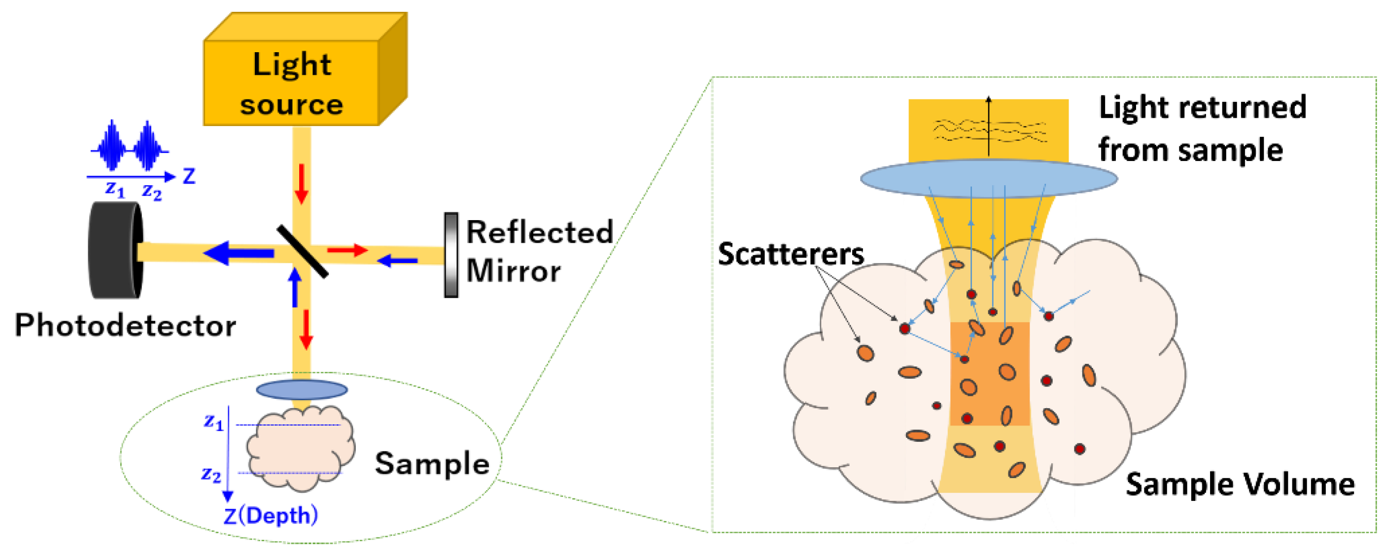
2.1. Principle

Figure 1 is a schematic diagram showing the origin of speckle in OCT. The principle of OCT is based on low-coherence measurements that visualize the tomographic structure from scattered and reflected light intensity information from a sample, which contains a large number of scatterers [3]. When the light illuminates the sample, multiple backward-scattering with random direction occurs due to the presence of scatterers in the sample volume. The light returning from one sample volume point is the sum of multiple scattering components, given by the following [4,5,10]:

$$\begin{array}{l}I={\displaystyle \sum _{n=1}^N{A}_n}\exp [-2ik(r+\Delta r_n)]\\ =\exp (-ik\cdot 2r){\displaystyle \sum _{n=1}^N{A}_n}\exp (-ik\cdot 2\Delta r_n)\end{array}$$

(1)

where I is the summation of multiple scattered light intensity, N is the number of scatterers in a sample volume point, n is the randomly scattered light caused by each scatterer, k is the wave number ($k=\frac{2\pi }{\lambda }$, λ is the wavelength), A_n and r are the amplitude and average optical pathlength for each scattering component, respectively, Δr_n is the pathlength difference, and (r + Δr_n) is the one-way optical pathlength. The superposition of multiple scattering components with random phases results in a reflected intensity fluctuation and granular texture presentation, degrading the image contrast in OCT.

Speckle, an inherent and specific characteristic in OCT, is random but definitive noise because the scatterers’ distribution does not change in time [11]. For speckle reduction, it is necessary to perform speckle decorrelation to change the speckle patterns on the same sample structure. To do so, we introduce an interesting source, a quasi-SC fiber laser, which has a tunable central wavelength, bandwidth, and spectral shape [30]. It is expected that this light source will be useful for achieving speckle decorrelation by different optical spectral bands.

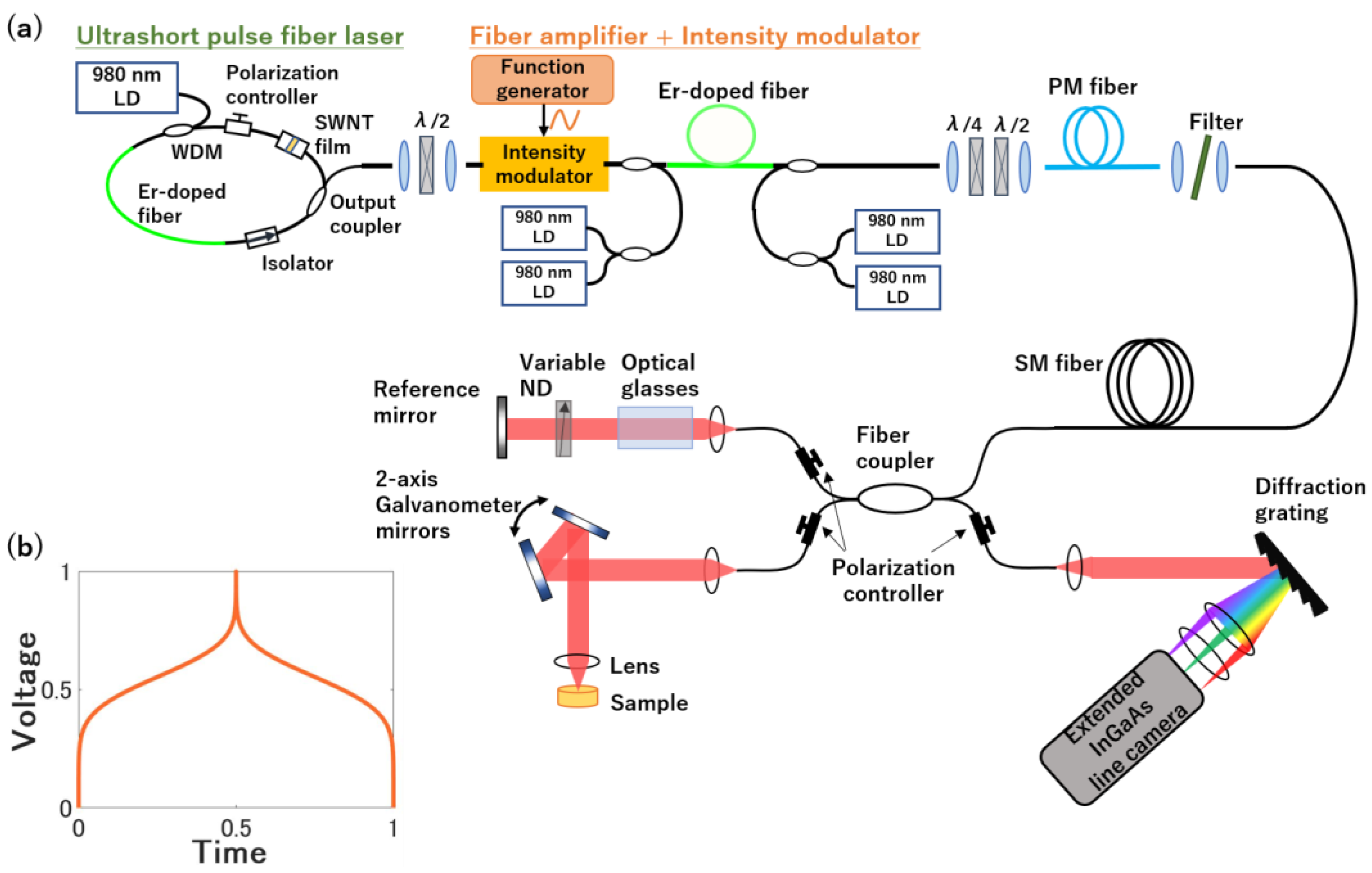
2.2. Experimental Setup

Figure 2a shows the experimental setup for speckle-reduced OCT using a quasi-SC fiber laser source. The experimental system is composed of a quasi-SC source, a reference arm, a sample arm, and a custom-built spectrometer, which are connected by a 50–50 fiber coupler.

For generation of a tunable optical spectrum, a quasi-SC fiber laser was developed based on wavelength-tunable Raman soliton generation and continuous soliton intensity modulation [30,34,35]. We used an ultra-short-pulse fiber laser as the seed pulse source. The output power was 23 mW, the repetition rate was 95.5 MHz, and the central wavelength was 1556 nm. The seed pulse was then amplified to the maximum power of 360 mW by an Er-doped fiber amplifier, and the pulse intensity was varied by using an electro-optical (EO) intensity modulator (LN81S-FC, Thorlabs, Newton, NJ, USA). A new Raman soliton was formed in a 300 m length of polarization-maintaining (PM) fiber. As the PM fiber input power was increased, the wavelength of the Raman soliton shifted more toward the longer wavelength side. The maximum wavelength and the wavelength shifting speed of the generated Raman soliton were determined by the maximum amplified intensity and the modulation frequency of intensity modulator, respectively. After a long pass filter, a wavelength-tunable Raman soliton was generated in a spectral window from 1600 nm to 1900 nm. When the modulation frequency was higher than the sampling frequency of the detection system, many shifted Raman solitons seemed to be generated at the same time. The detected spectrum was the superposition of these Raman solitons, appearing to be super-continuous, that is to say, a quasi-SC. In this quasi-SC generation, the modulation function determines the spectral shape. Actually, the modulation function determines the tuning speed of the Raman solitons at each wavelength. In order to generate Gaussian-shaped spectra, the design of the modulation function is important. When the slope of the modulation function was set to be gentle around the center wavelength, a larger number of Raman solitons were generated, and the integrated power of the solitons was greater. On the other hand, in the shorter and longer wavelength ranges, the slope of the modulation function was set to be steep, and the integrated power of the solitons was smaller. From the model calculations, we designed the modulation function shown in Figure 2b. We used a programmed function generated by a multifunction generator (WF1968, Nf, Yokohama, Japan) to modulate the pulse intensity. The modulation amplitude and offset affected the central wavelength and bandwidth, and a variable Gaussian spectral output could be achieved by adjusting the modulation amplitude and offset.

In the fiber coupler, the output light from the quasi-SC source was divided into the reference arm and sample arm, and the reflected light from the sample and reference mirror interfered with each other. To detect the interference signal, we used a custom-built spectrometer consisting of a 150 lines/mm blazed diffraction grating (015-200, Shimadzu, Kyoto, Japan), two focusing achromatic lenses (AC508-040-C and AC508-050-C, Thorlabs, Newton, NJ, USA), and a high-speed InGaAs line scan camera (SU1024LDH-2.2RT-0250/LC, Goodrich, Princeton, NJ, USA). The pixel number and line rate of the camera were 1024 pixels and 47 kHz, respectively. The detection spectral range was designed to be from 1400 to 2000 nm. The dispersion and polarization mismatches between the sample arm and reference arm were removed by using polarization controllers and inserting dispersion-compensating optical glasses in the reference arm.

3. Results

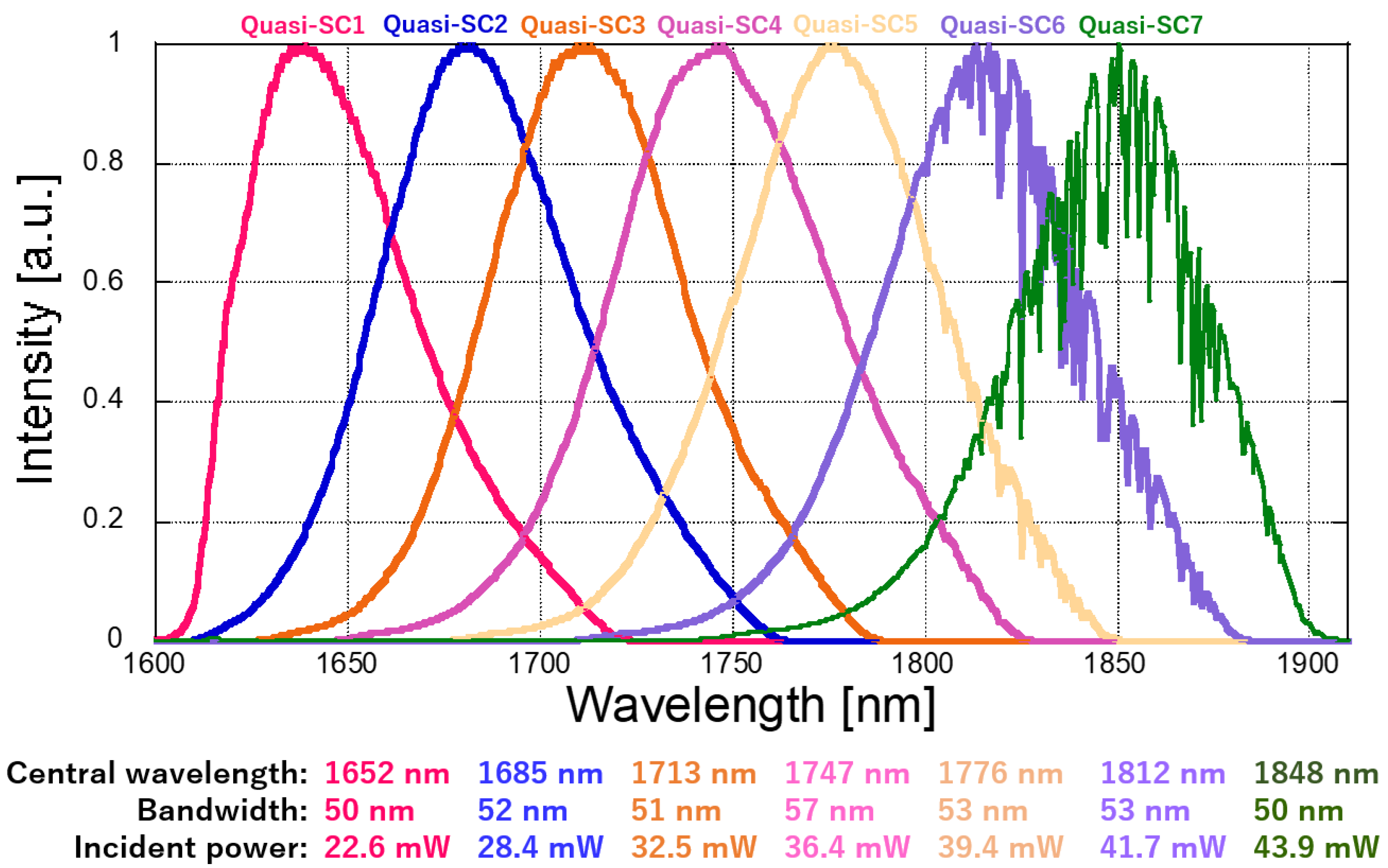
3.1. Tunable Quasi-SC Output

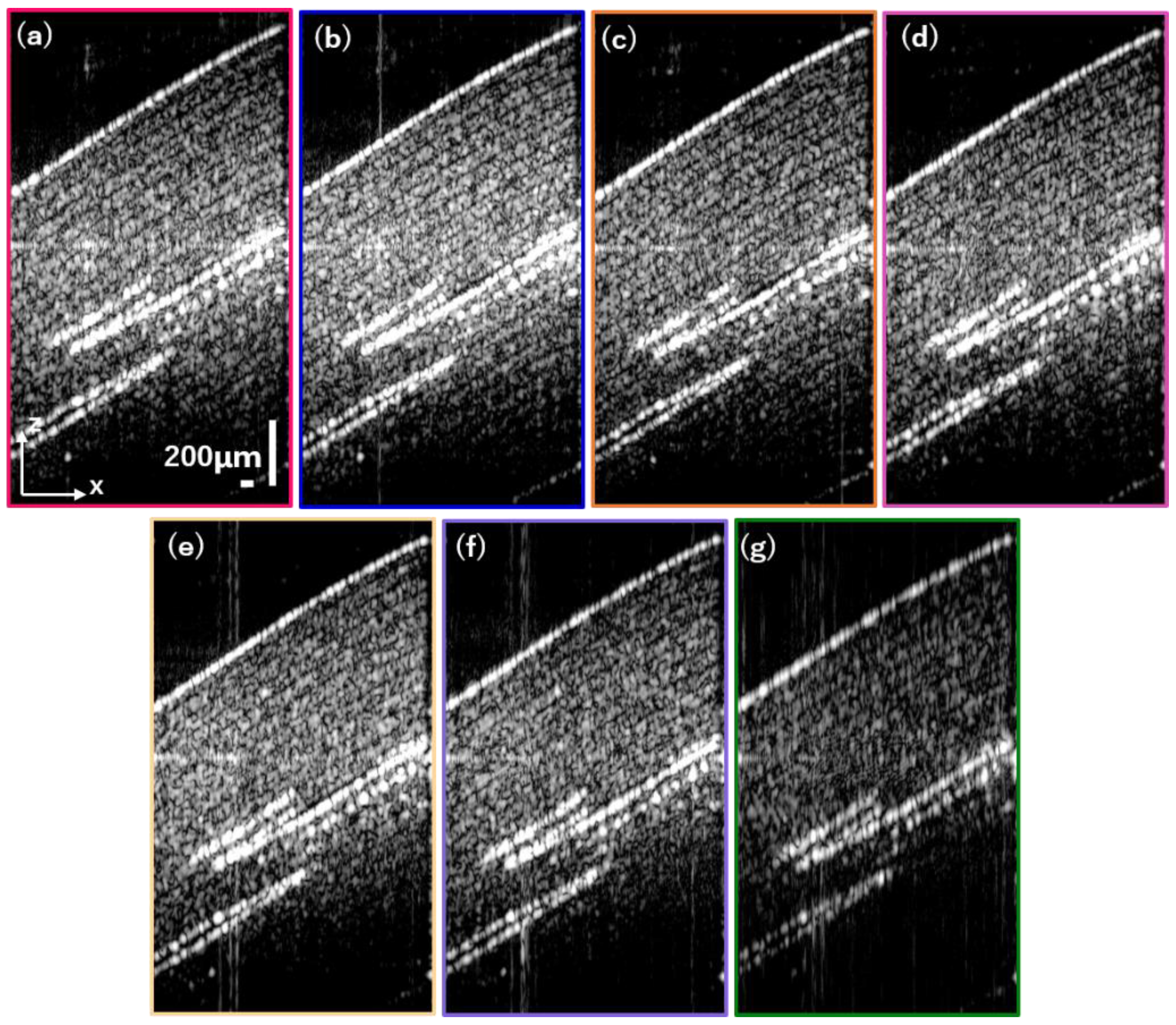
By adjusting the modulation amplitude and offset, seven Gaussian-like quasi-SC spectra, labeled sequentially as quasi-SC1 to quasi-SC7, were generated in the spectral band from 1600 nm to 1900 nm, as shown in Figure 3. They were centered at different wavelengths with different spectral bandwidths and output powers. The detailed values are also listed at the bottom of Figure 3.

We applied the above tunable quasi-SC output to an OCT system and examined the total system sensitivity and lateral resolution using a reflective mirror as a sample. Figure 4a shows the cross-sectional image for the sample of reflective mirror using quasi-SC1, and the interference signal is shown in Figure 4b. The total system sensitivities were 97 dB, including a 39-dB round-trip filter attenuation. The axial resolution was 24.1 μm, corresponding to 17.4 μm in biological tissue. We also examined the lateral resolution by the edge profile method.

Table 1. Characteristics of OCT imaging using quasi-SC1 to quasi-SC7.

	Quasi-SC1	Quasi-SC2	Quasi-SC3	Quasi-SC4	Quasi-SC5	Quasi-SC6	Quasi-SC7
Sensitivity (dB)	97	97	99	96	98	95	88
Axial resolution (μm) (in air) /(in tissue)	24.1/ 17.4	22.3/ 16.1	22.4/ 16.2	23.1/ 16.7	22.1/ 16.0	23.1/ 16.7	33.1/ 23.9
Lateral resolution (μm) (theoretical value) /(measured value)	30.2/ 31.9	30.8/ 32.3	31.4/ 32.6	32.0/ 33.1	32.5/ 34.2	33.2/ 36.2	33.8/ 41.7

summarizes the sensitivity and spatial resolution for each quasi-SC. The light source of quasi-SC1 to quasi-SC6 had similar high sensitivity (≥95 dB), close axial resolutions (around 17 μm), and lateral resolution (around 33μm). Quasi-SC7 at the longer wavelength side had worse sensitivity (<90 dB), the larger axial resolution (>22 μm in tissue), and lateral resolution (>40 μm) compared with quasi-SC1 to quasi-SC6 because of the design of the detection spectrometer.

3.2. Tape Stacks

Figure 5a–g shows a series of cross-sectional images obtained using quasi-SC1 to quasi-SC7. The OCT images consisted of 512 A-scans with 1024 pixels per scan, and the imaging time required for one cross-sectional frame was about 0.05 s. The corresponding frame rate was 20 frames/s. They have similar structures, and 20 or more layers were observed in the tape stacks, but the junctions between layers were not very clear due to the appearance of speckle patterns, especially in the image obtained using quasi-SC7 shown in Figure 5g because of the low imaging sensitivity in the longer wavelength region. We examined the correlation coefficients between the initial cross-section images, as shown in

Table 2. Correlation coefficients between initial cross-section images by quasi-SC 1–7.

	Quasi-SC1	Quasi-SC2	Quasi-SC3	Quasi-SC4	Quasi-SC5	Quasi-SC6	Quasi-SC7
Quasi-SC1	1
Quasi-SC2	0.825	1
Quasi-SC3	0.804	0.823	1
Quasi-SC4	0.795	0.786	0.836	1
Quasi-SC5	0.772	0.760	0.801	0.834	1
Quasi-SC6	0.767	0.760	0.786	0.800	0.840	1
Quasi-SC7	0.673	0.664	0.697	0.706	0.705	0.751	1

. The smaller the value of the coefficient is, the more uncorrelated speckle patterns there are. The greater the spectral difference between two quasi-SCs was, the better the de-correlation effect was. This indicates the effectiveness of spectral diversity in speckle decorrelation.

For speckle reduction, we utilized the compound average of the cross-sectional images shown in Figure 6. As shown in Figure 6, the contrast of speckle-reduced images became much better, and the junctions in the layer structure were observed more clearly. This result suggests successful improvement of the image quality using a tunable quasi-SC source with the spectral compounding method.

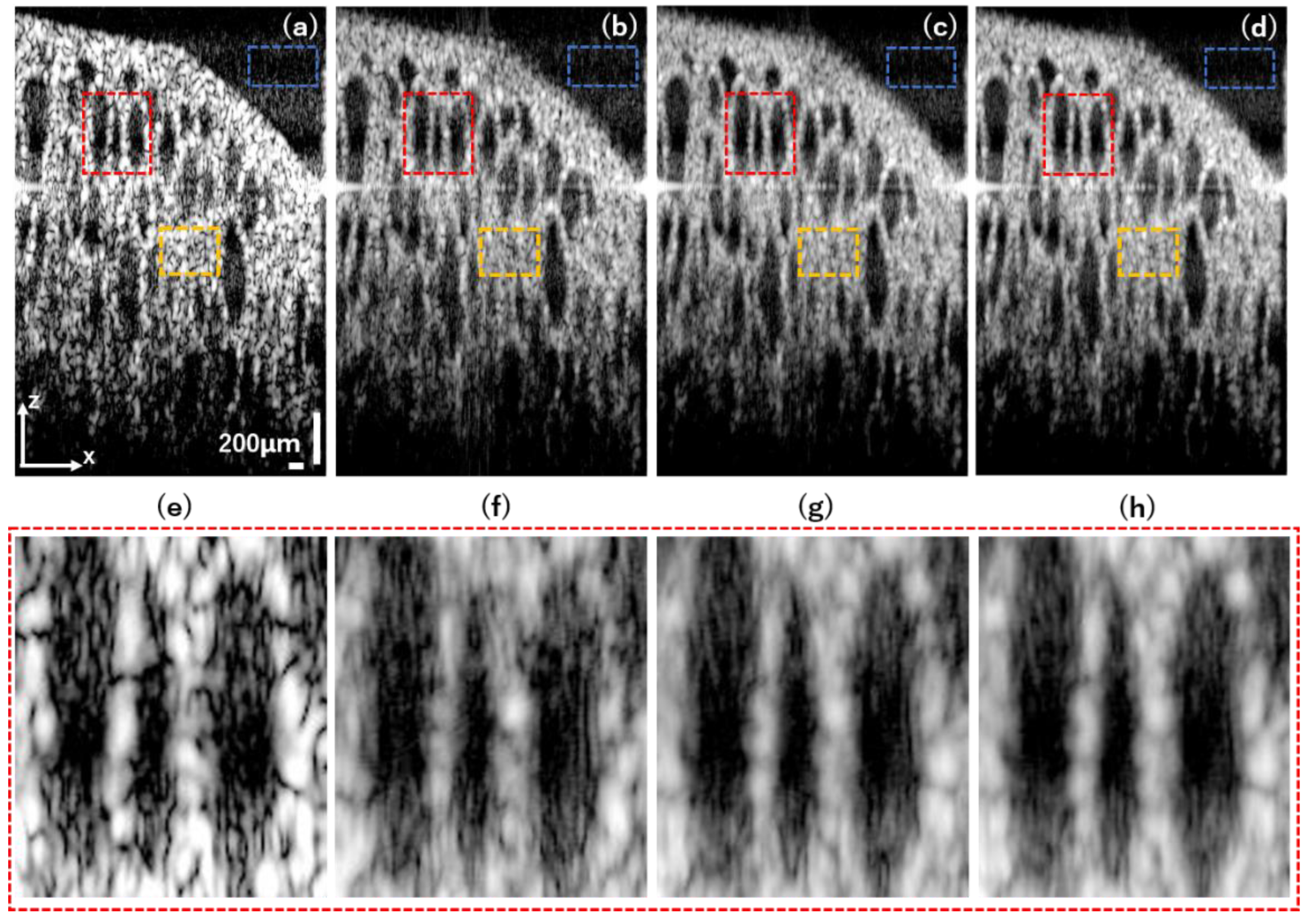
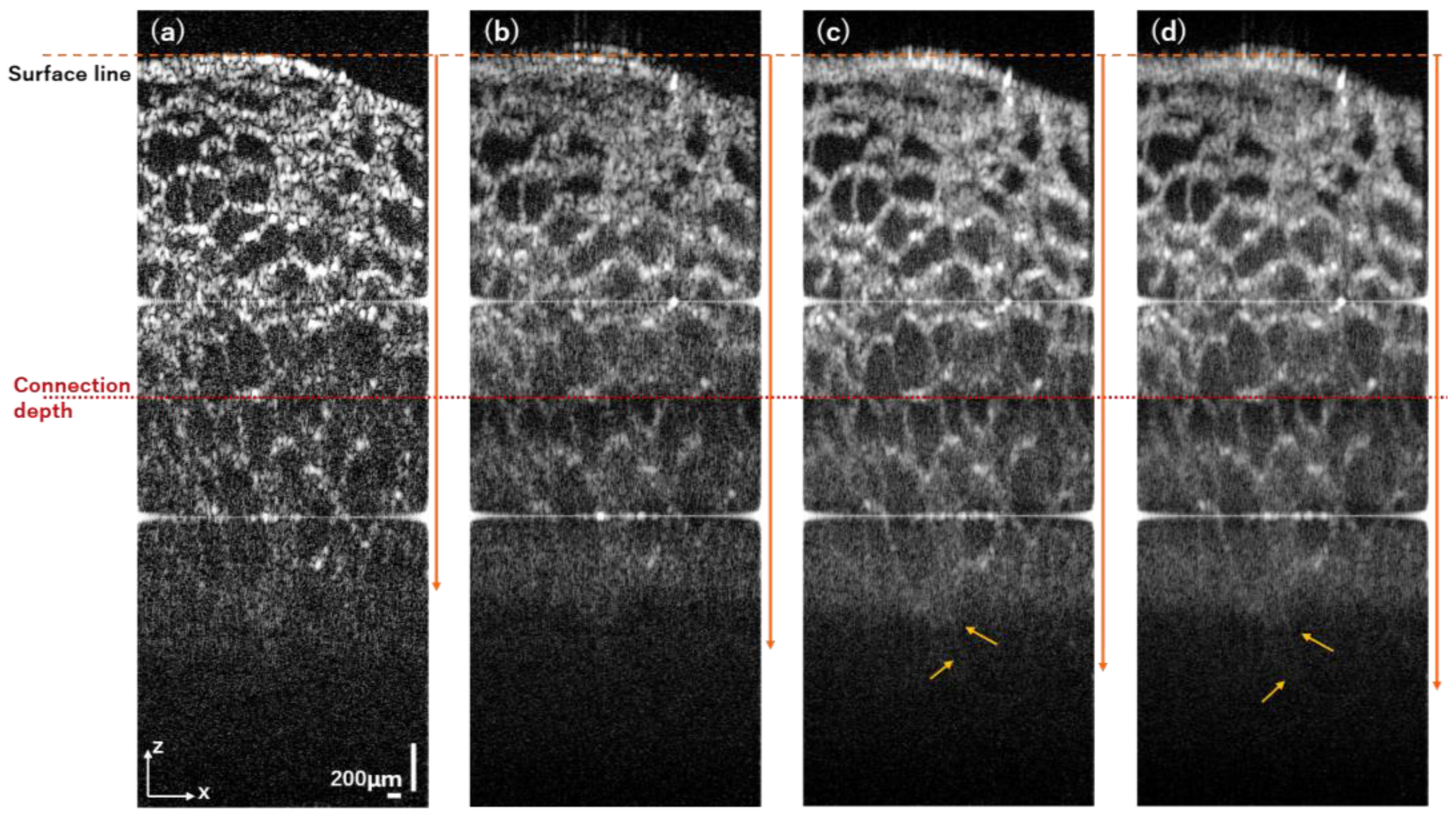
3.3. Pig Thyroid Gland

We also obtained initial and speckle-reduced OCT images of biological tissue, specifically pig thyroid gland. We used a fresh pig thyroid gland for each tissue imaging experiment. The gland tissue sample was prepared by fascia exfoliating and cutting into small pieces of approximately 1 cm in diameter and 0.5 cm in thickness. We also applied a medical coupling agent (SONO JELLY) to the surface of sample tissue for the high-quality transmission of optical waves. Figure 7a shows a cross-sectional image obtained with quasi-SC2. Figure 7b–d show speckle-reduced images with averaging numbers n = 3, 5, and 7, respectively. For the averaging number n = 3, we compounded the images obtained with quasi-SC1, quasi-SC4, and quasi-SC7. For the averaging number n = 5, we compounded the images obtained with quasi-SC2, quasi-SC3, quasi-SC4, quasi-SC5, and quasi-SC6. Figure 7e–h show enlarged images of the red rectangular regions in Figure 7a–d. From the images, we found that the whole structures of the pig thyroid gland were more clearly observed in speckle-reduced OCT images, and the image contrast looked much better as the averaging number increased.

In fact, there are many compounding combinations for each averaging number besides the averaging number n = 7. Figure 8 shows detailed structures of the pig thyroid gland with different combinations at different averaging numbers. For example, Figure 8a shows the compounded image averaged using quasi-SC1 and quasi-SC5, and Figure 8b shows the compounded image averaged using quasi-SC5 and quasi-SC6. The less the spectral overlapping between light sources is, the better the speckle suppression is. In addition, the quality of the compounded image is also related to the initial image contrast. And as the averaging number increases, the speckle-reduced image quality significantly improves.

We also compared the penetration depth in both initial images and speckle-reduced images. Figure 9a shows the connected image reconstructed by simple connection of two images obtained in shallow and deep regions using quasi-SC4. We set the middle point of top structure as the surface line and defined the penetration depth as the maximum depth at which we can distinguish a signal and background noise. The examined penetration depth of 1.54 mm was obtained by quasi-SC4. The similar connected images were obtained in the same way by other quasi-SCs. The maximum imaging depths for quasi-SC 1–3 were 1.31 mm, 1.44 mm, and 1.45 mm, respectively, because of a strong middle noise. The penetration depths for quasi-SC 5–7 were 1.46 mm, 1.40 mm, and 1.14 mm, respectively, due to a larger water absorption for biological tissue and a worse sensitivity at this wavelength range. Figure 9b shows the compound connected image with an averaging number of n = 3 by averaging the connected images with quasi-SC1, quasi-SC4, and quasi-SC7. Figure 9c shows the compound connected image with an averaging number of n = 5 by averaging the connected images with quasi-SC2, quasi-SC3, quasi-SC4, quasi-SC5, and quasi-SC6. Figure 9d shows the compound connected image with an averaging number of n = 7. The penetration depths were improved by the compound averaging method, and the new tissue structures appeared slightly in the deeper part in compound images with the averaging numbers of n = 5 and n = 7, indicated by the yellow arrow. The maximum imaging depths for the compound images with the averaging numbers of n = 3, n = 5, and n = 7 were 1.70 mm, 1.82 mm, and 1.82 mm, respectively.

We finally examined image quality by using the image metrics signal-to-noise ratio (SNR), contrast (C), and contrast-to-noise ratio (CNR). Here, we chose the blue rectangular region as the background area, and the red and yellow regions as two signal areas, shown in Figure 7a. SNR, C, and CNR can be calculated using the following equations:

$$SNR={\overline{I}}_{signal}/\sqrt{{\sigma }^2{}_{signal}}$$

(2)

$$C={\overline{I}}_{signal}/{\overline{I}}_{background}$$

(3)

$$CNR=\left({\overline{I}}_{signal}-{\overline{I}}_{background}\right)/\sqrt{{\sigma }^2{}_{signal}+{\sigma }^2{}_{background}}$$

(4)

where $\overline{I}$ and ${\sigma }^2$ represent the average intensity and standard deviation of the selected regions. We obtained the values of the image metrics by means of two signal areas, shown in

Table 3. Image metrics of initial images and speckle-reduced images.

	Initial Images Using Quasi-SCs							Speckle-Reduced Images
	Quasi-SC1	Quasi-SC2	Quasi-SC3	Quasi-SC4	Quasi-SC5	Quasi-SC6	Quasi-SC7	n = 3	n = 5	n = 7
SNR (dB)	3.25	2.93	2.83	2.61	2.45	1.25	1.06	4.01	4.99	5.24
C	18.53	20.64	21.50	20.43	19.48	5.51	4.67	21.11	30.74	41.90
CNR (dB)	3.11	2.89	2.80	2.59	2.30	0.80	0.62	3.96	4.99	5.24
Imaging depth (mm)	1.31	1.44	1.45	1.54	1.46	1.40	1.14	1.70	1.82	1.82

. By comparing parameters, we confirmed that the image quality was improved by the spectral compound averaging method, and the image quality was much improved as the averaging number increased.

4. Discussion

In this paper, we demonstrated that a tunable quasi-SC source configured for OCT allowed us to obtain uncorrelated speckle patterns for speckle reduction. The presented scheme combines the advantages of the hardware and software methods mentioned before, and does not require post-algorithmic processing to reduce the image acquisition time, nor does it require additional experimental equipment, which enhances the stability of the system. Because the wavelength and bandwidth of the quasi-SC source are variable, it is possible to realize both high-resolution single imaging using ultra-wideband light and low-speckle compound imaging using multiple spectra at different wavelengths.

However, there was a tradeoff between the axial resolution and the degree of speckle reduction because of the limited spectral band used, 1600 nm to 1900 nm. A better speckle reduction result requires higher averaging numbers n and smaller overlaps between spectra, but a higher axial resolution needs a wider bandwidth spectrum. In addition, the axial resolution increases or decreases, because the axial resolution is determined by the central wavelength and bandwidth and differs for each individual quasi-SC. In the experiment, we set the modulation amplitude and offset as parameters to adjust the central wavelength and bandwidth manually. Nevertheless, implementing a quasi-SC provides an approach to improve the performance of OCT without the need for additional devices, instruments, and postprocessing.

For future optimizations, the enlargement of wavelength-tunable range, which allows us to obtain more and wider quasi-SC spectra, and the implementation of a high NA confocal lens in the sample arm may help us to enhance both axial resolution and lateral resolution. We would also be able to apply our scheme to the real-time imaging for living samples, if we realize the whole computer-controlled system for fast modulation adjustment of a quasi-SC source and corresponding quick acquisition of OCT images.

5. Conclusions

In conclusion, this is the first attempt at speckle-reduced OCT using one light source with a tunable spectral output via the compounding method. We obtained speckle-reduced images of two samples, tape stacks and pig thyroid gland. The compounded images had a more clear structure as the speckle noise was suppressed. As the averaging number increased and the difference with the wavelength range became greater, the image quality improved. The quantitative parameters SNR, C, and CNR were increased by at least 2 dB, 20, and 2 dB, respectively, which corroborated the improved speckle-reduced imaging results. We also confirmed the improvement in penetration depth for the developed speckle-reduced OCT.

References

1. Huang, D.; Swanson, E.A. Optical coherence tomography. Science 1991, 254, 1178–1181. [Google Scholar] [CrossRef] [PubMed]
2. Schmitt, J.M. Optical coherence tomography (OCT): A review. IEEE J. Sel. Top. Quantum Electron. 1999, 5, 1205–1215. [Google Scholar] [CrossRef]
3. Drexler, W.; Fujimoto, J.G. Optical Coherence Tomography: Technology and Applications, 2nd ed.; Springer: Berlin, Germany, 2015; pp. 22–35. [Google Scholar]
4. Goodman, J.W. Speckle Phenomena in Optics: Theory and Applications, 2nd ed.; Society of Photo Optical: Washington, DC, USA, 2010; pp. 11–20. [Google Scholar]
5. Tearney, G.J.; Brezinski, M.E. In Vivo Endoscopic Optical Biopsy with Optical Coherence Tomography. Science 1997, 276, 2037–2039. [Google Scholar] [CrossRef] [PubMed]
6. Podoleanu, A.G.; Rogers, J.A. Three dimensional OCT images from retina and skin. Opt. Express 2000, 7, 292–298. [Google Scholar] [CrossRef]
7. Pierce, M.C.; Strasswimmer, J. Advances in optical coherence tomography imaging for dermatology. J. Investig. Dermatol. 2004, 123, 458–463. [Google Scholar] [CrossRef]
8. Herz, P.R.; Chen, Y. Ultrahigh resolution optical biopsy with endoscopic optical coherence tomography. Opt. Express 2004, 12, 3532–3542. [Google Scholar] [CrossRef]
9. Triesscheijn, M.; Baas, P. Non-invasive monitoring of morphologic changes after mTHPC mediated photodynamic therapy (PDT) in a mouse tumor model using optical coherence tomography (OCT). Cancer Res. 2005, 65, 1118. [Google Scholar]
10. Freitas, A.Z.; Zezell, D.M. Imaging carious human dental tissue with optical coherence tomography. J. Appl. Phys. 2006, 99, 024906. [Google Scholar] [CrossRef]
11. Li, X.; Yin, J. High-resolution coregistered intravascular imaging with integrated ultrasound and optical coherence tomography probe. Appl. Phys. Lett. 2010, 97, 133702. [Google Scholar] [CrossRef]
12. Vakoc, B.J.; Dai, F. Cancer imaging by optical coherence tomography: Preclinical progress and clinical potential. Nat. Rev. Cancer 2012, 12, 363–368. [Google Scholar] [CrossRef]
13. Choi, W.J.; Zhi, Z. In vivo OCT microangiography of rodent iris. Opt. Lett. 2014, 39, 2455–2458. [Google Scholar] [CrossRef]
14. Schmitt, J.M.; Xiang, S.H. Speckle in optical coherence tomography. J. Biomed. Opt. 1999, 4, 95–105. [Google Scholar] [CrossRef] [PubMed]
15. Bashkansky, M.; Reintjes, J. Statistics and reduction of speckle in optical coherence tomography. Opt. Lett. 2000, 25, 545–547. [Google Scholar] [CrossRef] [PubMed]
16. Karamata, B.; Hassler, K. Speckle statistics in optical coherence tomography. J. Opt. Soc. Am. A 2005, 22, 593–596. [Google Scholar] [CrossRef] [PubMed]
17. Desjardins, A.E.; Vakoc, B.J. Angle-resolved Optical Coherence Tomography with sequential angular selectivity for speckle reduction. Opt. Express 2007, 15, 6200–6209. [Google Scholar] [CrossRef] [PubMed]
18. Říha, R.; Marques, M.J. Direct en-face, speckle-reduced images using angular-compounded Master–Slave optical coherence tomography. J. Opt. 2020, 22, 055302. [Google Scholar] [CrossRef]
19. Pircher, M.; Götzinger, E. Speckle reduction in optical coherence tomography by frequency compounding. Biomed. Opt. Express 2003, 8, 565–569. [Google Scholar] [CrossRef]
20. Magnain, C.; Wang, H. En face speckle reduction in optical coherence microscopy by frequency compounding. Opt. Lett. 2016, 41, 1925–1928. [Google Scholar] [CrossRef]
21. Li, R.; Yin, H. Speckle reducing OCT using optical chopper. Opt. Express 2020, 28, 4021–4031. [Google Scholar] [CrossRef]
22. Liba, O.; Lew, M.D. Speckle-modulating optical coherence tomography in living mice and humans. Nat. Commun. 2017, 8, 15845. [Google Scholar] [CrossRef]
23. Adler, D.C.; Ko, T.H. Speckle reduction in optical coherence tomography images by use of a spatially adaptive wavelet filter. Opt. Lett. 2004, 29, 2878–2880. [Google Scholar] [CrossRef] [PubMed]
24. Lippok, N.; Nielsen, P. Single-shot speckle reduction and dispersion compensation in optical coherence tomography by compounding fractional Fourier domains. Opt. Lett. 2013, 38, 1787–1789. [Google Scholar] [CrossRef] [PubMed]
25. Ozcan, A.; Bilenca, A. Speckle reduction in optical coherence tomography images using digital filtering. J. Opt. Soc. Am. 2007, 24, 1901–1910. [Google Scholar] [CrossRef] [PubMed]
26. Yu, H.; Gao, J. Probability-based non-local means filter for speckle noise suppression in optical coherence tomography images. Opt. Express 2016, 41, 994–997. [Google Scholar] [CrossRef] [PubMed]
27. Cuartas-Vélez, C.; Restrepo, R. Volumetric non-local-means based speckle reduction for optical coherence tomography. Biomed. Opt. Express 2018, 9, 3354–3372. [Google Scholar] [CrossRef] [PubMed]
28. Zhang, X.; Li, Z. Denoising algorithm of OCT images via sparse representation based on noise estimation and global dictionary. Opt. Express 2022, 30, 5788–5802. [Google Scholar] [CrossRef] [PubMed]
29. Gong, G.; Zhang, H. Speckle noise reduction algorithm with total variation regularization in optical coherence tomography. Opt. Express 2015, 23, 24699–24712. [Google Scholar] [CrossRef]
30. Chen, Y.; Yamanaka, M. Tunable quasi-supercontinuum generation in a 1.7 µm spectral band for spectral domain optical coherence tomography. Opt. Contin. 2023, 2, 1941–1949. [Google Scholar] [CrossRef]
31. Nishizawa, N.; Kawagoe, H. Wavelength dependence of ultrahigh-resolution optical coherence tomography using supercontinuum for biological imaging. IEEE J. Sel. Top. Quantum Electron. 2018, 25, 1–15. [Google Scholar] [CrossRef]
32. Ishida, S.; Nishizawa, N. Quantitative comparison of contrast and imaging depth of ultrahigh-resolution optical coherence tomography images in 800-1700 nm wavelength region. Biomed. Opt. Express 2012, 3, 282–294. [Google Scholar] [CrossRef]
33. Chen, Y.; Yamanaka, M.; Kitajima, S.; Nishizawa, N. Speckle Reduction by Frequency Compounding in 1.7 μm Optical Coherence Tomography using Tunable Quasi-Supercontinuum Laser Source. In Proceedings of the Conference on Lasers and Electro-Optics, JW3B.152, San Jose, CA, USA, 18 May 2022. [Google Scholar]
34. Sumimura, K.; Ohta, T. Quasi-super-continuum generation using ultrahigh-speed wavelength-tunable soliton pulses. Opt. Lett. 2008, 33, 2892–2894. [Google Scholar] [CrossRef] [PubMed]
35. Sumimura, K.; Ohta, T. Quasi-supercontinuum generation using 1.06 μm ultrashort-pulse laser system for ultrahigh-resolution optical-coherence tomography. Opt. Lett. 2010, 35, 3631–3633. [Google Scholar] [CrossRef] [PubMed]
Figure 1. Schematic diagram showing origin of speckle in OCT.
Photonics 10 01338 g001
Figure 2. (a) Experiment setup for SD-OCT using quasi-SC fiber laser source. (b) Intensity modulation function for Gaussian-shaped quasi-SC generation.
Photonics 10 01338 g002
Figure 3. Spectra of quasi-SC1 to quasi-SC7 and detailed information for each quasi-SC output.
Photonics 10 01338 g003
Figure 4. (a) Cross-sectional OCT image of a reflective mirror and (b) interference signal of OCT using quasi-SC1.
Photonics 10 01338 g004
Figure 5. (ag) Series of initial OCT images of tape stacks obtained using quasi-SC1 to quasi-SC7.
Photonics 10 01338 g005
Figure 6. Compound averaged image of tape stacks.
Photonics 10 01338 g006
Figure 7. (a) OCT image of pig thyroid gland using quasi-SC2. Compounded images with (b) averaging number n = 3, (c) averaging number n = 5, (d) averaging number n = 7. (eh) Enlarged images of red rectangular positions in (ad). The blue rectangular region is the background area we choose for each image, and the red and yellow regions are the two signal areas to calculate the image metrics in Table 3.
Photonics 10 01338 g007
Figure 8. Enlarged images of pig thyroid gland with (a) averaging number of n = 2 using quasi-SC1,5, (b) averaging number of n = 2 using quasi-SC5,6, (c) averaging number of n = 3 using quasi-SC1,2,4, (d) averaging number of n = 3 using quasi-SC1,3,5, (e) averaging number of n = 4 using quasi-SC1,2,3,4, (f) averaging number of n = 4 using quasi-SC1,3,4,6, (g) averaging number of n = 5 using quasi-SC1,2,3,4,5, (h) averaging number of n = 5 using quasi-SC1,2,4,5,6, (i) averaging number of n = 6 using quasi-SC1,2,3,4,5,6, (j) averaging number of n = 6 using quasi-SC1,2,3,4,5,7.
Photonics 10 01338 g008
Figure 9. (a) Connected cross-sectional images by quasi-SC4. Compounded images of connected works with averaging number of (b) n = 3, (c) n = 5, and (d) n = 7. The orange arrows represent the maximum imaging depth for each image.
Photonics 10 01338 g009