Turbulence Aberration Restoration Based on Light Intensity Image Using GoogLeNet

Abstract

Adaptive optics (AO) is an effective method to compensate the wavefront distortion caused by atmospheric turbulence and system distortion. The accuracy and speed of aberration restoration are important factors affecting the performance of adaptive optics correction. In recent years, an AO correction method based on a convolutional neural network (CNN) has been proposed for the non-iterative extraction of light intensity image features and recovery of phase information. This method can directly predict the Zernike coefficient of the wavefront from the measured light intensity image and effectively improve the real-time correction ability of the AO system. In this paper, a turbulence aberration restoration based on two frames of a light intensity image using GoogLeNet is established. Three depth scales of GoogLeNet and different amounts of data training are tested to verify the accuracy of Zernike phase difference restoration at different turbulence intensities. The results show that the training of small data sets easily overfits the data, while the training performance of large data sets is more stable and requires a deeper network, which is conducive to improving the accuracy of turbulence aberration restoration. The restoration effect of third-order to seventh-order aberrations is significant under different turbulence intensities. With the increase in the Zernike coefficient, the error increases gradually. However, there are valley points lower than the previous growth for the 10th-, 15th-, 16th-, 21st-, 28th- and 29th-order aberrations. For higher-order aberrations, the greater the turbulence intensity, the greater the restoration error. The research content of this paper can provide a network design reference for turbulence aberration restoration based on deep learning.

1. Introduction

When a laser propagates in atmospheric turbulence, the phase and intensity perturbations caused by atmospheric turbulence effect seriously damage the beam quality [1]. Adaptive optics (AO) is a powerful means to compensate wavefront distortions caused by the aberration of the optical system, atmospheric turbulence or other factors [2]. The traditional method of compensating aberration in an adaptive optics system is to measure distortion wavefront using a wavefront sensor and drive wavefront corrector using a wavefront controller. The existence of a wavefront sensor makes the structure of the whole adaptive optics system complex and expensive, and its application field is difficult to expand and popularize. Another correction method without a wavefront sensor is to find the optimal driver of the corrector by iteration of an optimization algorithm [3,4,5,6]. This method has a simple structure, but a slow convergence rate becomes a technological bottleneck. According to the wavefront recovery theory of Gerchberg-Saxton [7], it is proposed that the phase distribution of the optical field on the input planes can be uniquely determined by measuring two optical intensities. The phase diversity principle developed by R. Gonsalves [8] also points out that phase can be uniquely determined by using an intensity image in the focal plane and a defocus plane through maximum likelihood estimation. Accordingly, the adaptive optical compensation without a wavefront sensor can be regarded as the process of restoring the distorted phase by measuring the intensity of light. The nonlinear matching model of an intensity image and aberration coefficient is established offline, and the distortion wavefront can be predicted directly by the model when the intensity image is measured online. In this way, the system has a simple structure and no iterative calculation is needed, which can improve the timeliness of the system.

In 1990, Angel et al. [9] established a matching model of light intensity information and Zernike coefficients based on a three-layer feedback neural network to correct the piston and tilt aberration in the wavefront distortion of a multi-telescope system. Sandler and Barrett et al. [10,11] used the 1.5m telescope of Philips Laboratory of the US Air Force based on the BPNN algorithm to realize the observation of real stars by combining the intensity distribution of the focal plane and defocusing plane, and the Zernike order reached 11 orders. However, higher-order aberration correction has not been studied, because the parameters of input nodes will increase nonlinearly as the spot expands, and the training process of the network itself becomes extremely difficult.

Deep convolutional neural networks (CNNs) are a new type of network and have the ability to automatically effectively learn the nonlinear relationship between input and output. During the past two years, deep learning technology has been developing rapidly. CNNs have been applied to the field of image recognition in applications such as medical image recognition [12,13], human motion recognition [14,15], street view recognition [16,17], and vehicle detection [18] and further applied to audio and video recognition [19,20], where it achieved very good results. CNNs can be set up using the appropriate convolution layer, pooling layer and full connection layer. A CNN can automatically extract image features and can thus be used as a general feature extraction tool and applied to aberration identification from intensity images in the optical communication and imaging environment.

Since 2017, there have been some attempts to use deep learning techniques for the restoration of distorted wavefronts. T. V. Nguyen et al. [21] proposed a fully automatic technique to obtain aberration-free quantitative phase imaging in digital holographic microscopy based on deep learning and proposed a novel method that combines a supervised deep learning technique with CNN and Zernike polynomial fitting. F. Xiao et al. [22] proposed a deep learning method to restore degraded retinal images, and the method directly learned an end-to-end mapping between the blurred and restored retinal images. S. Lohani et al. [23,24] designed an optical feedback network making use of machine learning techniques and demonstrated via simulations its ability to correct for the effects of turbulent propagation on optical modes. S. W. Paine [25] used machine learning operating on a point-spread function to determine a good initial estimate of the wavefront, and the trained convolutional neural network provided good initial estimates in the presence of simulated detector noise and is more effective than using many random starting guesses for large amounts of wavefront error. H. Ma [26] proposed a novel compensation technique based on AlexNet, which is trained by using large data sets of two intensity images that are measured in-focus and out-of-focus and Zernike coefficients for the distortions as inputs. Y. Nishizaki et al. [27] experimentally demonstrated a variety of image-based wavefront sensing architectures that can directly estimate Zernike coefficients of aberrated wavefronts from a single intensity image by using Xception. H. Guo [28] presented a novel real-time non-iterative phase-diversity wavefront sensing method that successfully established the nonlinear mapping between intensity images and the corresponding aberration coefficients by using LeNet. K. Wang [29] verified the correction effect for a turbulence pool and the feasibility for a real atmospheric turbulence environment using a U-Net and a CNN containing a residual block. In recent years, many advanced networks for wavefront restoration have also been developed [30,31,32].

The above studies are aimed at the realization of an end-to-end CNN from a light intensity image to the phase. Compared with image classification and recognition, the task of directly predicting Zernike coefficient quantitative labels from light intensity images is a more complex feature extraction process. The depth of the network and the size of the data set will be the influencing factors that need to be tested and discussed. In this paper, the turbulence aberration compensation ability based on GoogLeNet is tested. Considering the factors such as different turbulence intensities, different data set sizes and different network depths, the models in various cases are trained, and the optimized training model is tested. We try to test and analyze the recovery performance of the convolutional neural network for different order Zernike coefficients of turbulence aberrations. We hope that the research in this paper will be helpful for the combination of deep learning and adaptive optics and provide a reference for improving the deep model of phase restoration.

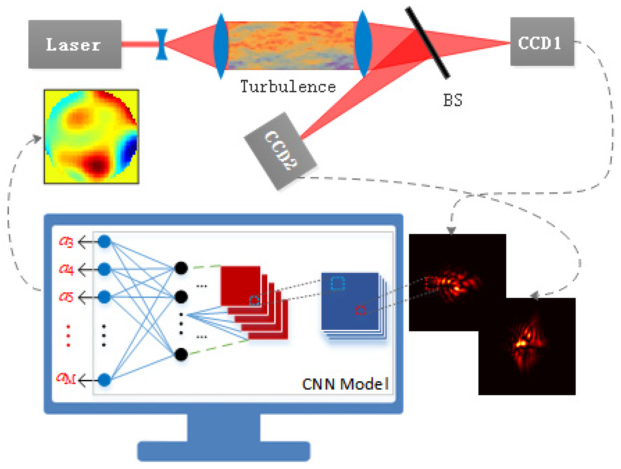
2. Related Principle and Method

2.1. Turbulence Aberration Restoration Model Based on CNN

The diagram for the turbulence aberration restoration model based on a CNN is shown in Figure 1. The distortion wavefront $\varphi (x,y)$ of atmospheric turbulence is expressed by orthogonal Zernike polynomials as expansion basis functions [33]:

$$\varphi (x,y)={\displaystyle \sum _{i=1}^{\infty }{a}_i}{z}_i(x,y)$$

(1)

where $a_i$ is the coefficient of the $i$th Zernike polynomial and $z_i(x,y)$ is the $i$th Zernike polynomial. According to Kolmogorov turbulence theory, the covariance matrix $C$ of the coefficient vector $A=\{a_1,a_2,\dots ,a_M\}$ of the Zernike polynomial can be obtained by [34]

$$〈a_i{a}_j〉=c_{ij}{\left(\frac{D}{r_0}\right)}^{5/3}$$

(2)

where $D$ is the pupil aperture and $r_0$ is the Fried parameter [35]. For the plane wave, $r_0={(0.423k^2{C}_n^{2}z)}^{-3/5}$, where $k=\frac{2\pi }{\lambda }$, $\lambda$ is the wavelength, and $C_n^2$ is the atmospheric turbulence structure constant. The singular value decomposition of the C matrix [36] is as follows:

$$\begin{array}{l}C=VS{V}^T\\ A=VB\end{array}$$

(3)

where $S$ is a diagonal matrix, $V$ is the coefficient of the Karhumen–Loeve polynomial and $B$ is the coefficient of the phase $\phi (x,y)$. Then the distortion wavefront of atmospheric turbulence in accordance with the Kolmogorov turbulence spectrum can be obtained from the Formula (1) using the coefficient matrix A.

When a plane wave enters the pupil and propagates through a turbulent medium, the complex amplitude with turbulence aberration is $U_0(x_0,y_0)$. The light wave is imaged on two CCDs in the far field, and the intensity images of the focal plane and the defocus plane are obtained. The complex amplitude of the focal plane light field $U_1(f_x,f_y)$ can be obtained by Fourier transform of the complex amplitude of the incident light field $U_0(x_0,y_0)$:

$$U_1(f_x,f_y)==C_1\Im \left(U_0(x_0,y_0)\right)$$

(4)

where $C_1$ is a complex constant and $\Im$ is the Fourier transform operator. The complex amplitude of the defocusing surface $U_2(f_x,f_y)$ can be expressed as

$$U_2(f_x,f_y)=C_2\Im (U_0(x_0,y_0)\exp (-i\phi (x,y)))$$

(5)

where $\phi (x,y)$ is a defocus phase.

2.2. Structure of Convolutional Neural Network

The CNN model implemented in this study follows the idea of GoogLeNet Inception V2 [37], which was the winner of ILSVRC-2014. The architecture of GoogLeNet we implemented for turbulence aberration reconstruction (TAR-GoogLeNet) is shown in Figure 2. GoogLeNet uses a modular structure, which is easy to add and modify. The structure of the Inception module is shown in Figure 2. The Inception module is made up of 1 × 1 convolutions, 3 × 3 convolutions, 5 × 5 convolutions and 3 × 3 max pooling layers. One of the biggest differences in GoogLeNet is that there are two sigmoid branches in the middle as auxiliary loss functions. In this way, we can test the training effect of three different depth networks. In the following section, we call these three outputs S1, S2 and S3, respectively. In training, the losses of the two branches are empirically added to the total loss function S in a ratio of 0.3:

S = 0.3 × S1 + 0.3 × S2 + S3

(6)

When we use GoogLeNet to perform aberration restoration, the original input image is 224 × 224 × 2, where 2 refers to the normalized light intensity image in focus and out of focus, and the image is pre-processed using the zero-mean method (subtracting the mean from each pixel of the image). Finally, after the sigmoid activation, the Zernike coefficient of the distorted wavefront is obtained in our study, so a vector of length $N$ is obtained. The output is the Zernike coefficient $\{a_3,a_4,\dots ,a_{35}\}$ of aberration. The turbulence distortion compensation process based on a CNN can be considered as a nonlinear mapping transformation model of intensity images and the Zernike coefficients of the distortion:

$$\{a_1,a_2,\dots ,a_N\}=f_{CNN}(I_1(x,y),I_2(x,y_y))$$

(7)

2.3. Data Preparation

We use mature algorithms to simulate the generation of training image data. This process mainly includes the generation of aberration distortion of random atmospheric turbulence disturbance, the generation of intensity speckle images of the far-field focal plane and defocus plane and the introduction of noise. A series of Zernike coefficients and light intensity images obtained through this process will be used as training data for neural network training.

Considering the plane wave incident on an ideal clear pupil, the amplitude of the light field is expressed as

$$A(x,y)=\left\{\begin{array}{c}1\begin{array}{ccc}& \sqrt{x^2+y^2}\le D/2& \end{array}\\ 0\begin{array}{ccc}& \sqrt{x^2+y^2}>D/2& \end{array}\end{array}\right.$$

(8)

The phase of atmospheric turbulence disturbance is $\varphi (x,y)$, and the light field affected by atmospheric turbulence can be expressed as

$$U_0(x,y)=A(x,y)e^{i\varphi (x,y)},$$

(9)

where $\varphi (x,y)$ is the unknown aberration function in actual wavefront recovery. When generating training data, the phase $\varphi (x,y)$ is generated by the method described in Section 2.1. The focal plane complex amplitude $U_1(f_x,f_y)$ and the defocusing plane complex amplitude $U_2(f_x,f_y)$ can be calculated separately by

$$\begin{array}{l}{U}_1(f_x,f_y)=\Im (e^{i\varphi (x,y)})\\ U_2(f_x,f_y)=\Im (e^{i[\varphi (x,y)+{\varphi }_d(x,y)]})\end{array}$$

(10)

where ${\varphi }_d(x,y)$ is the known defocus aberration, which is generated by ${\varphi }_d(x,y)=a_4{Z}_4(x,y)$. The intensity image matrix of the focal plane $I_1(x,y)$ and non-focal plane $I_2(x,y)$ can be obtained by

$$\begin{array}{l}{I}_1(x,y)={\left|U_1(f_x,f_y)\right|}^2\\ I_2(x,y)={\left|U_2(f_x,f_y)\right|}^2\end{array}$$

(11)

In preparation for the training, Zernike coefficients $\{a_3,a_4,\dots ,a_{35}\}$ in agreement with Kolmogorov turbulence distortion were randomly generated, and the corresponding intensity images in focus $I_1(x,y)$ and out of focus $I_2(x,y)$ were obtained by the corresponding calculation. The calculated light intensity image is 256 × 256 pixels, the initial grid spacing Δx is 0.01m, there are 60 points on the initial light field diameter and the far-field spatial frequency spacing is 1/(256Δx). The light intensity image is cropped to 224 × 224 as network input. In order to ensure the stability of the training model, we needed to prepare a lot of data. Three sets of data of different sizes were prepared, and the amount of data we prepared is described in

Table 1. Generated training data description.

Turbulence Intensity $(\mathit{D}/{\mathit{r}}_0)$	$\mathit{D}/{\mathit{r}}_0$ Interval	Data Volume for Each Interval (Set)	Total Data Volume (Set)
From 1 to 15	1	100	1500
From 1 to 15	1	1000	15,000
From 1 to 15	1	10,000	15,0000

.

2.4. The Training Method

In the training process, the stochastic gradient descent method (SGD) is needed to minimize the cross-entropy loss function. The loss function is

$$loss={{\displaystyle \sum _i\left(y_i-y_{-}predicte{d}_i\right)}}^2+{\displaystyle \sum _i\left|y_i-y_{-}predicte{d}_i\right|},$$

(12)

where $y_i$ is the actual Zernike coefficients and $y\_predicte{d}_i$ is the predicted ones in our work. The SGD algorithm is used to train the model so that the learning parameters and updates of the samples are used in each iteration. The learning parameters and updates of each generation [38] can be expressed as follows:

$$V_{i+1}=\mu V_{{}^t}-\alpha \nabla loss\left(W_i\right),$$

(13)

$$W_{t+1}=W_t+V_{t+1},$$

(14)

where t is the number of iterations, $W_t$ is the parameters of t, $V_t$ is the increment of t, $\alpha$ is the learning rate, $\mu$ is the weights of the previous update and $\nabla loss\left(W_i\right)$ is the partial differentiation of the loss function. The learning rate is set as 0.001.

3. Experiment Results and Analysis

3.1. Loss Value Results of GoogLeNet Training and Testing

We implemented the CNN training in Python 3.6 with tensorflow 1.3.0. The algorithm was run on a desktop PC with an Intel Core i9-7900X CPU at 3.3GHz and 16GB DDR4 RAM. We trained three data sets separately, and the loss value of the training process changed as shown in Figure 3. Figure 3a–c show the training result of sets of 1500, 15,000 and 150,000 samples, and the black, red and blue curves are the results of outputs S1, S2 and S3, respectively. Figure 3d gives a comparison of the output result S for three sample sets. It can be seen from the figures that in the training process, the loss function of the S2 model of the 1500 data set decreases best, and the S3 model performs well for 15,000 and 150,000 data sets. For the S1 model, the loss function does not converge with the iteration for the three data sets.

The trained model was tested on the test sample set, and the results in the same form are shown in Figure 4. Note that there are no duplicate sample data between the test set and the training set. It can be seen from the figures that the test results of the 1500 and 15,000 data sets are overfitted. The result of 150,000 data set test is very good, especially for the S3 output, for which the loss function is the best. As shown in Figure 4d, for the total test comparison, the 150,000 data set training is the best.

3.2. Some Samples of Turbulence Aberration Restoration

After training the CNN, we tested the performance of the trained network. First, the results of three different distortions with D/r₀ = 1, 5, 10 and 15 are intuitively given in Figure 5a–d. The atmospheric wavefronts for D/r₀ = 1, 5, 10 and 15 were randomly generated. For each sample, the real wavefront, the wavefront predicted by GoogLeNet S3 and the Zernike coefficients are shown. We can see that the predicted wavefront shape is very close to the real wavefront, but the error near the edge is large. This could be due to the limited accuracy of the simulation grid, so the RMS difference of the wavefront is relatively large.

3.3. Results of Turbulence Aberration Restoration for Different Cases of D/r₀

In order to further test the restoration performance of Zernike coefficients of turbulence aberration by GoogLeNet S3, we randomly generated 100 sets of data for each D/r₀ case to test. The value of D/r₀ is set from 1 to 15 and the interval is 1. Figure 6 shows the error map of the prediction and the true Zernike coefficients of different Zernike orders and different turbulence intensity D/r₀ values. The ordinate represents different Zernike orders, the abscissa represents the turbulence intensity D/r₀ and the results between every two green lines represent 100 random cases under the turbulence intensity marked by the abscissa. It can be seen from Figure 6 that when the turbulence intensity is very small, the error of phase difference restoration of each order is small. As the turbulence intensity increases, the color of the map becomes brighter and brighter, that is, the restoration error becomes larger and larger; Zernike orders 3~7 have small restoration errors under different turbulence intensities. With the increase in Zernike order, the overall restoration error tends to be larger and larger, but there are some dark stripes here in Zernike orders 15, 16, 21, 22, 28 and 29.

By averaging 100 groups of data in each D/r₀ case in Figure 7, we can obtain the statistical results of the Zernike coefficient error of each Zernike order under different turbulence intensities, as shown in Figure 7a. As can be seen from Figure 7a, with the increase in turbulence intensity, the restoration error of Zernike aberration of each order is basically increasing; with the increase in Zernike order, the restoration errors under different turbulence intensities maintain the same broken-line trend. In order to more clearly see the restoration effect of each order aberration, we further statistically average the restoration error of each order Zernike aberration under different turbulence intensities, as shown in Figure 7b. The results shown in Figure 7b indicate that the restoration effect of third-order to seventh-order Zernike aberration is very good under the turbulence conditions calculated in this study. With the increase in the Zernike coefficient, the error gradually increases. However, we can clearly see that there are valley points lower than the previous growth for the 10th-, 15th-, 16th-, 21st-, 28th- and 29th-order aberrations. The third order to the seventh order are low-order aberrations, the 10th and 21st are spherical aberrations and the 15th/16th and the 28th/29th are comas.

Turbulence aberration is the superposition of Zernike aberrations of various orders, and different wavefront aberrations have different effects on the focus distribution. In order to explore the reasons for the above results, the focus intensity distribution of 3 ~ 35 single-order Zernike aberrations is given in Figure 8, and the given coefficient of each order aberration is a one-unit value. The aberration is expressed as a two-dimensional polynomial orthogonal to the continuous functions $Z_n^m$ of radial variables n and angular variables m in the circular domain. The two-dimensional Zernike polynomial is expressed in the form of only one order $Z_k$. The corresponding relationship between $Z_k$ and $Z_n^m$ is shown in the marks in the upper left corner and the upper right corner in Figure 8. As can be seen from Figure 8, the light intensity distribution of orders 3–8 is relatively concentrated, and the spot pattern is relatively simple. With the increase in N, m decreases, and the distribution of the spot pattern becomes relatively clear and simple. The larger m is, the more seriously the spot is broken, the more complex the pattern is and the more complex and difficult to distinguish the contour is. Figure 9 shows the error map with radial variables n and angular variables m. It can be seen from Figure 9 that the light intensity pattern on the left and right sides is symmetrical about m = 0, and the error map also shows the trend of symmetry about m = 0. According to Figure 9 and Figure 8, the more concentrated the light intensity is, the simpler the spot pattern is and the smaller the error is. In the opposite case, the spot is seriously broken, and the more complex the pattern is, the greater the error is.

4. Conclusions

In this study, we implemented 3rd~35th-order turbulence aberration restoration using GoogLeNet. The effects of different data set sizes and network depth on the restoration accuracy were tested. The GoogLeNet models with data set sizes of 150,000, 15,000 and 150,000 and three depths were tested. The results show that the training of small data sets easily overfits data, while the training performance of large data sets is more stable and requires a deeper network, which is conducive to improving the accuracy of turbulence aberration restoration. The prediction errors of 3rd~35th-order Zernike coefficients were analyzed in detail. The results show that the recovery effect of third-order to seventh-order aberrations is significant under different turbulence intensities; with the increase in the Zernike coefficient, the error increases gradually. However, there are valley points lower than the previous growth for the 10th-, 15th-, 16th-, 21st-, 28th- and 29th-order aberrations. The third order to the seventh order are low-order aberrations, the 10th and 21st are spherical aberrations and the 15th/16th and the 28th/29th are comas. By comparing the far-field intensity patterns of Zernike aberrations, it is found that the more concentrated the light intensity is, the simpler the spot pattern is and the smaller the error is. In the opposite case, the spot is seriously broken, and the more complex the pattern is, the greater the error is. The research content of this paper can provide a network design reference for turbulence aberration restoration based on deep learning.

The method of extracting light intensity image features and recovering phase information through deep learning is an end-to-end phase sensing method, which can effectively improve the real-time performance of optical systems and is expected to enhance their practical application value. However, there is still a certain gap related to the application requirements of high-precision wavefront recovery. A convolutional neural network has the ability to self-extract image features. The ability to extract features is largely related to the size of the convolution kernel, that is, the receptive field. Determining how to improve the network design and improve the ability to restore complex high-order aberration of spot patterns is a big problem. Therefore, the next work will continue to explore a more appropriate network structure to improve the recovery accuracy, robustness and interpretability.

References

1. Strohbehn, J. Laser Beam Propagation in the Atmosphere; Springer: Berlin/Heidelberg, Germany, 1990. [Google Scholar]
2. Tyson, R. Principles of Adaptive Optics, 3rd ed.; CRC Press: Boca Raton, FL, USA, 2010. [Google Scholar]
3. Vorontsov, M.; Carhart, G.; Ricklin, J.C. Adaptive phase-distortion correction based on parallel gradient-descent optimization. Opt. Lett. 1997, 22, 907–909. [Google Scholar] [CrossRef]
4. Song, H.; Fraanje, R.; Schitter, G.; Kroese, H.; Vdovin, G.; Verhaegen, M. Model-based aberration correction in a closed-loop wavefront-sensor-less adaptive optics system. Opt. Express 2010, 18, 24070–24084. [Google Scholar] [CrossRef] [PubMed] [Green Version]
5. Yang, H.; Soloviev, O.; Verhaegen, M. Model-based wavefront sensorless adaptive optics system for large aberrations and extended objects. Opt. Express 2015, 23, 24587–24601. [Google Scholar] [CrossRef]
6. Dong, B.; Li, Y.; Han, X.-L.; Hu, B. Dynamic Aberration Correction for Conformal Window of High-Speed Aircraft Using Optimized Model-Based Wavefront Sensorless Adaptive Optics. Sensors 2016, 16, 1414. [Google Scholar] [CrossRef] [PubMed] [Green Version]
7. Gerchberg, R.W.; Saxton, W.O. A practical algorithm for the determination of phase from image and diffraction plane pictures. Optik 1972, 35, 237–250. [Google Scholar]
8. Gonsalves, R.A. Phase retrieval and diversity in adaptive optics. Opt. Eng. 1982, 21, 829–832. [Google Scholar] [CrossRef]
9. Angel, J.R.P.; Wizinowich, P.; Lloyd-Hart, M.; Sandler, D. Adaptive optics for array telescopes using neural-network techniques. Nature 1990, 348, 221–224. [Google Scholar] [CrossRef]
10. Sandler, D.G.; Barrett, T.K.; Palmer, D.A.; Fugate, R.Q.; Wild, W.J. Use of a neural network to control an adaptive optics system for an astronomical telescope. Nature 1991, 351, 300–302. [Google Scholar] [CrossRef]
11. Barrett, T.K.; Sandler, D.G. Artificial neural network for the determination of Hubble Space Telescope aberration from stellar images. Appl. Opt. 1993, 32, 1720–1727. [Google Scholar] [CrossRef] [Green Version]
12. Suzuki, K. Overview of deep learning in medical imaging. Radiol. Phys. Technol. 2017, 10, 257–273. [Google Scholar] [CrossRef]
13. Hamwood, J.; Alonso-Caneiro, D.; Read, S.A.; Vincent, S.J.; Collins, M.J. Effect of patch size and network architecture on a convolutional neural network approach for automatic segmentation of OCT retinal layers. Biomed. Opt. Express 2018, 9, 3049–3066. [Google Scholar] [CrossRef] [PubMed] [Green Version]
14. Liu, M.; Liu, H.; Chen, C. Enhanced skeleton visualization for view invariant human action recognition. Pattern Recognit. 2017, 68, 346–362. [Google Scholar] [CrossRef]
15. Janidarmian, M.; Roshan, F.A.; Radecka, K.; Zilic, Z. A Comprehensive Analysis on Wearable Acceleration Sensors in Human Activity Recognition. Sensors 2017, 17, 529. [Google Scholar] [CrossRef] [PubMed] [Green Version]
16. Tsai, T.H.; Cheng, W.H.; You, C.W.; Hu, M.C.; Tsui, A.W.; Chi, H.Y. Learning and Recognition of On-Premise Signs From Weakly Labeled Street View Images. IEEE Trans. Image Process. 2014, 23, 1047–1059. [Google Scholar] [CrossRef] [PubMed]
17. Hebbalaguppe, R.; Garg, G.; Hassan, E.; Ghosh, H.; Verma, A. Telecom Inventory Management via Object Recognition and Localisation on Google Street View Images. In Proceedings of the 2017 IEEE Winter Conference on Applications of Computer Vision, Santa Rosa, CA, USA, 24–31 March 2017. [Google Scholar]
18. Manana, M.; Tu, C.; Owolawi, P.A. A survey on vehicle detection based on convolution neural networks. In Proceedings of the 2017 3rd IEEE International Conference on Computer and Communications, Chengdu, China, 13–16 December 2017. [Google Scholar]
19. Ringeval, F.; Valstar, M.; Jaiswal, S.; Marchi, E.; Lalanne, D.; Cowie, R.; Pantic, M. AV+EC 2015:The First Affect Recognition Challenge Bridging Across Audio, Video, and Physiological Data. In Proceedings of the International Workshop on Audio/visual Emotion Challenge, Brisbane, Australia, 26 October 2015. [Google Scholar]
20. Valstar, M.; Gratch, J.; Ringeval, F.; Lalanne, D.; Torres, M.T.; Scherer, S.; Stratou, G.; Cowie, R.; Pantic, M. AVEC 2016: Depression, Mood, and Emotion Recognition Workshop and Challenge. In Proceedings of the 6th International Workshop on Audio/Visual Emotion Challenge, Amsterdam, The Netherlands, 16 October 2016. [Google Scholar]
21. Nguyen, T.; Bui, V.; Lam, V.; Raub, C.B.; Chang, L.-C.; Nehmetallah, G. Automatic phase aberration compensation for digital holographic microscopy based on deep learning background detection. Opt. Express 2017, 25, 15043–15057. [Google Scholar] [CrossRef]
22. Fei, X.; Zhao, J.; Zhao, H.; Yun, D.; Zhang, Y. Deblurring adaptive optics retinal images using deep convolutional neural networks. Biomed. Opt. Express 2017, 8, 5675–5687. [Google Scholar] [CrossRef] [Green Version]
23. Lohani, S.; Glasser, R.T. Turbulence correction with artificial neural networks. Opt. Lett. 2018, 43, 2611–2614. [Google Scholar] [CrossRef]
24. Lohani, S.; Knutson, E.M.; O’Donnell, M.; Huver, S.D.; Glasser, R.T. On the use of deep neural networks in optical communications. Appl. Opt. 2018, 57, 4180–4190. [Google Scholar] [CrossRef]
25. Paine, S.W.; Fienup, J.R. Machine learning for improved image-based wavefront sensing. Opt. Lett. 2018, 43, 1235–1238. [Google Scholar] [CrossRef] [Green Version]
26. Ma, H.; Liu, H.; Qiao, Y.; Li, X.; Zhang, W. Numerical study of adaptive optics compensation based on Convolutional Neural Networks. Opt. Commun. 2019, 433, 283–289. [Google Scholar] [CrossRef]
27. Nishizaki, Y.; Valdivia, M.; Horisaki, R.; Kitaguchi, K.; Saito, M.; Tanida, J.; Vera, E. Deep learning wavefront sensing. Opt. Express 2019, 27, 240–251. [Google Scholar] [CrossRef] [PubMed]
28. Wu, Y.; Guo, Y.; Bao, H.; Rao, C. Sub-Millisecond Phase Retrieval for Phase-Diversity Wavefront Sensor. Sensors 2020, 20, 4877. [Google Scholar] [CrossRef] [PubMed]
29. Wang, K.; Zhang, M.; Tang, J.; Wang, L.; Hu, L.; Wu, X.; Li, W.; Di, J.; Liu, G.; Zhao, J. Deep learning wavefront sensing and aberration correction in atmospheric turbulence. PhotoniX 2021, 2, 8. [Google Scholar] [CrossRef]
30. Xu, Y.; Guo, H.; Wang, Z.; He, D.; Tan, Y.; Huang, Y. Self-Supervised Deep Learning for Improved Image-Based Wave-Front Sensing. Photonics 2022, 9, 165. [Google Scholar] [CrossRef]
31. Wang, M.; Guo, W.; Yuan, X. Single-shot wavefront sensing with deep neural networks for free-space optical communications. Opt. Express 2021, 29, 3465–3478. [Google Scholar] [CrossRef]
32. Li, Y.; Yue, D.; He, Y. Prediction of wavefront distortion for wavefront sensorless adaptive optics based on deep learning. Appl. Opt. 2022, 61, 4168–4176. [Google Scholar] [CrossRef]
33. Wang, J.Y.; Silva, D.E. Wave-front interpretation with Zernike polynomials. Appl. Opt. 1980, 19, 1510–1518. [Google Scholar] [CrossRef]
34. Noll, R.J. Zernike polynomials and atmospheric turbulence. J. Opt. Soc. Am. A 1976, 66, 207–211. [Google Scholar] [CrossRef]
35. Li, Z.; Li, X. Fundamental performance of transverse wind estimator from Shack-Hartmann wave-front sensor measurements. Opt. Express 2018, 26, 11859–11876. [Google Scholar] [CrossRef]
36. Roddier, N.A. Atmospheric wavefront simulation using Zernike polynomials. Opt. Eng. 1990, 29, 1174–1180. [Google Scholar] [CrossRef]
37. Szegedy, C.; Liu, W.; Jia, Y.; Sermanet, P.; Reed, S.; Anguelov, D.; Erhan, D.; Vanhoucke, V.; Rabinovich, A. Going Deeper with Convolutions. In Proceedings of the IEEE Conference on Computer Vision and Pattern Recognition, Boston, MA, USA, 7–12 June 2015; pp. 1–9. [Google Scholar]
38. Goodfellow, I.; Bengio, Y.; Courville, A. Deep Learning; People’s Posts and Telecommunications Publishing House: Beijing, China, 2017. [Google Scholar]
Figure 1. The diagram for turbulence aberration restoration model based on CNN.
Photonics 10 00265 g001
Figure 2. The architecture of GoogLeNet for turbulence aberration restoration. The structure of the Inception module in GoogLeNet is shown in the dotted box.
Photonics 10 00265 g002
Figure 3. The loss value curve for the training process on the training data set of (a) 1500 (b) 15,000 and (c) 150,000. (d) The loss value curve comparison of the output result S for three training data set.
Photonics 10 00265 g003
Figure 4. The loss value curve for the test process on the test data set of (a) 1500 (b) 15,000 and (c) 150,000. (d) The loss value curve comparison of the output result S for three test data set.
Photonics 10 00265 g004
Figure 5. Four turbulence aberration samples for (a) D/r0 = 1, (b) D/r0 = 5, (c) D/r0 = 10, (d) D/r0 = 15: the first column is the real wavefront, the second column is the predicted wavefront by GoogLeNet S3 and the third column is the comparison of Zernike coefficients between the real wavefront and the predicted wavefront.
Photonics 10 00265 g005
Figure 6. The error map of prediction and real Zernike coefficients of different Zernike orders for D/r0 = 1~15.
Photonics 10 00265 g006
Figure 7. The statistical results of the Zernike coefficient error of each Zernike order: (a) in the case of different turbulence intensities, the error is counted as a broken line graph; (b) in the case of different turbulence intensities, the error is counted as a bar.
Photonics 10 00265 g007
Figure 8. The far-field focal plane intensity pattern of single-order aberration orders 3–35.
Photonics 10 00265 g008
Figure 9. Zernike coefficient error map with radial variables n and angular variables m.
Photonics 10 00265 g009