Real Aperture Continuous Terahertz Imaging System and Spectral Refinement Method

Abstract

In order to meet the increasing demand of non-destructive testing (NDT) in engineering practice, a continuous terahertz NDT platform based on linear scanning has been developed, with a center frequency of 154 GHz and a bandwidth of 56 GHz. This system combines frequency modulation continuous wave (FMCW) radar technology with a continuous scanning structure, as well as a data acquisition platform to provide a non-contact detection method; this is highly efficient and compensates for the shortcomings of traditional methods such as microwave, X-ray, ultrasonic, and others in safety inspection and special detection. In addition, a signal processing method of spectral refinement and correction is proposed in this paper for accurate thickness measurement. The results show that the method has a high accuracy for ABS, PVC, and ceramic matrix composites. By extracting the characteristic parameters, the detection and imaging of prefabricated defects, such as debonding and bubbles in composite materials, have been successfully achieved. This helps to evaluate the internal state of the inspected object more intuitively and further meets the requirements of industrial NDT.

1. Introduction

With the extensive application of new manufacturing technologies and new materials in the industrial field, the problems of inspecting quality and evaluating reliability have become increasingly prominent [1,2]. In recent years, terahertz technology has been proven to have strong application prospects and development potential in industrial non-destructive testing (NDT). This area has gradually become a research hotspot due to its various advantages, such as the fact that it is low-energy, harmless to the human body, non-contact, and has the ability to penetrate non-metallic materials, amongst others [3,4,5].

Terahertz waves lie between millimeter waves and infrared light on the electromagnetic spectrum, placing them within the transitional zone from electronics technology to optical technology [6,7]. However, they are not fully applicable to microwave and optical theory research; therefore, their generation and detection are limited [8]. It was not until the 1980s—with the development of technologies such as photoconductive antennas (PCAs), optical rectification (OR), and electro-optical sampling (EOS)—that the research into terahertz waves made some progress [9,10,11,12]. Various bodies of research show that terahertz waves have a high application value in wireless communication [13,14], safety inspection [15,16,17], biomedical imaging [18], composite material detection [19,20,21], art protection [22], etc.

In general, terahertz imaging systems are categorized as either active or passive. However, even in the terahertz band, with frequencies up to 100 GHz or more, passive detection still reduces the detection sensitivity and image resolution, while the radiation source of active systems can overcome these deficiencies. Therefore, the application of terahertz imaging technology in NDT mainly relies on active systems. According to the type of emission source, terahertz imaging systems are subdivided into two forms of radiation: pulsed wave and continuous wave. Representative devices are the terahertz time-domain spectrometer (THz-TDS) and frequency-modulated continuous wave (FMCW) radars [23,24,25,26]. The former is a technique used for NDT through analyzing the terahertz spectrum, which is reflected, transmitted, and scattered by the measured object. The spectral resolution determines the identification accuracy of the fingerprint spectrum, and a shorter coherent wavelength means that there is a higher longitudinal resolution, which is crucial for the detection of extremely small-size defects. However, the THz-TDS also has insurmountable limitations. Although femtosecond laser technology has made great progress in recent years, drawbacks such as the complex structure of the system, low detection efficiency, and tedious operation limit the application and popularization of the THz-TDS, meaning that it is not suitable for rapid detection scenarios [27]. In contrast, the sensor scheme based on a frequency-modulated continuous wave (FMCW) has the characteristics of high integration, miniaturization, and fast imaging speed, meaning that it is favored in engineering applications [28].

In recent years, many universities and research institutes have conducted research on FMCW radars and achieved certain results. NASA’s Jet Propulsion Laboratory (JPL), which is committed to the development of high-performance FMCW imaging systems, has introduced two systems in the frequency ranges of 576~604.8 GHz and 662.4~691.2 GHz for safety inspection, and it is researching a 95 GHz FMCW Doppler radar for space exploration [15,29]. The Pacific Northwest National Laboratory (PNNL) is dedicated to terahertz radar imaging with sparse arrays and reconstruction algorithms, and the designed imaging system has a bandwidth of only 19.2 GHz [30]. The Fraunhofer Institute for High-Frequency Physics and Radar Techniques (FHR) has developed an imaging system with a frequency range of 44 GHz, which uses an inverse synthetic aperture radar (ISAR) algorithm for imaging [31]. The SynView Head-300, produced by a German company, is one of the few devices currently used in the field of NDT, with a frequency range of 90 GHz [32]. Many research groups have studied signal and image processing algorithms based on this system. Terahertz FMCW imaging technology has also been studied in Sweden, China, and Spain, as well as other countries. Most of the above systems use the ISAR algorithm for imaging. For special equipment or composite material inspection where a higher accuracy is required, further research should be conducted.

In this paper, a linear terahertz FMCW scanning system is constructed, which is suitable for the non-contact detection of multilayer non-metallic materials, including thickness measurement and defect detection. The scanning system includes the terahertz sensor, three linear actuators, a control platform, and a human–computer interaction module. In this paper, the key contents of the system are introduced, and the test results are given to verify its detection ability. The main contributions of this paper are as follows.

First, combined with terahertz sensing technology, a set of continuous terahertz imaging platforms is built. By connecting the scanner and the data acquisition system, the real aperture terahertz imaging of continuous scanning is obtained.

Second, due to traditional frequency modulation (FM) signal processing methods having a low resolution accuracy and low efficiency, a complex resolving bandpass filter is constructed for signal processing and feature extraction. The effectiveness of the method is verified through simulation and comparison experiments.

Finally, the proposed continuous terahertz detection system is used to detect thermal protection structures in the aerospace field and successfully localize the defect locations.

2. FMCW Theory and System Description

2.1. FMCW Radar and Measuring Principle

According to the operating mode of the transmitting source, terahertz continuous wave (CW) systems can be divided into single-frequency continuous wave (SFCW), step-frequency-modulated continuous wave (SFMCW), and linear-frequency-modulated continuous wave (LFMCW) [28]. SFCW means that the transmission frequency of the signal source contains only one component. Therefore, it is generally believed that the SFCW system has no resolution in the distance direction and can only perform two-dimensional imaging [33]. Due to the presence of the FM cycle, the SFMCW system is required to dwell for one FM cycle at each detection position and then conduct a point-to-point scan to obtain the fully sampled data [28]. In contrast, the LFMCW system is more popular because of its short scanning time and fast imaging speed [34]. Figure 1 shows the principle of the measurement of the LFMCW system. The terahertz radar emits waves with a linearly varying frequency. Then, the reflected signals are captured by the system. These signals are shifted in time; therefore, their current frequency is also shifted compared to the transmitted signal.

The transmitted signal $S_{\mathrm{T}}\left(t\right)$ and the reflected signal $S_{\mathrm{R}}\left(t\right)$ can be represented by the following formulas:

$$S_{\mathrm{T}}\left(t\right)=A_{\mathrm{t}}\mathit{exp}\left[j2\pi \left(f_{0}t+\frac{1}{2}K{t}^2\right)\right]$$

(1)

$$S_{\mathrm{R}}\left(t\right)=A_{\mathrm{r}}\exp \left\{j2\pi \left[f_0\left(t-\Delta t\right)+\frac{1}{2}K{\left(t-\Delta t\right)}^2\right]\right\}$$

(2)

where $A_{\mathrm{t}}$ and $A_{\mathrm{r}}$ represent the amplitudes of transmitted and reflected signals, respectively, $f_0$ is the initial frequency, $B$ is the sweep frequency bandwidth, $t_{\mathrm{s}}$ is the period of a sweep cycle, $K=B/t_s$ is the chirp rate, and $\Delta t$ is the time offset caused by the distance of the measured target.

As shown in Figure 1, these signals produce a beat frequency $\mathsf{\Delta }f$ at the output of the mixer that is proportional to the propagation length. The formula for calculating the range domain can be obtained as follows:

$$d=c{t}_{\mathrm{s}}∆f/2nB$$

(3)

where $c$ is the speed of light and $n$ is the refractive index of the transmission medium ($n=1$ in the air). As the FM signal changes periodically, according to the Fast Fourier Transform (FFT) theory, the minimum frequency interval that the frequency can be resolved within in the observation window $t_{\mathrm{s}}$ is reciprocal of the observation time. Therefore, the range resolution of FMCW sensing theoretically depends on the bandwidth, which can be expressed by the following formula:

$$\delta =c/2nB$$

(4)

2.2. System Description

The proposed FMCW scanner is a complete imaging system, which is composed of the terahertz sensor, three linear actuators, a control platform, and a human–computer interaction module. The terahertz sensor, produced by the company TRILITEC in Germany, works in the frequency range of 126 GHz to 182 GHz, which includes a horn antenna with a set of lenses placed in front of the horn. Efficient illumination and the finest resolution can be ensured by placing the sample at the focal point of the lenses. Figure 2a,b shows the architecture of the terahertz imaging system and the linear scanning process. The workflow of the terahertz sensor is shown in Figure 2c. First, a voltage-controlled oscillator (VCO) is driven by a ramp generator to generate a fast saw-tooth low-frequency sweep signal. The low-frequency sweep signal is amplified through a frequency doubling link to become the transmission signal, TX, part of which is radiated into the air by the antenna, and the other part is directed straight into the mixer. With a focusing lens, the energy of this signal is concentrated in the focal plane for propagation. When the transmitted signal encounters a different material bonding layer, it returns to the terahertz source in the same path and is called the reflected signal, RX. Finally, the reflected signal and the other part of the transmitted signal are down-converted by a mixer and finally recorded as an intermediate frequency (IF) signal by an analog-to-digital converter (ADC). The frequency doubling link is mainly acquired through the use of Schottky diodes. The Schottky diode is a special diode with a high switching speed and low noise performance, which is widely used in microwave and millimeter wave bands for the wireless communication, radar, and measurement. In the frequency doubling link, the input signal is applied to the forward bias end of the Schottky diode, and the frequency of the input signal can be multiplied by the non-linear characteristics of the diode. In the mixer, the Schottky diode is used as a non-linear element to generate the product and difference frequencies of the input signal, where the product frequency is the product of the frequencies of two input signals and the difference frequency is the difference in the frequencies of the two input signals. This system mainly performs downward mixing.

This modulation method is equivalent to an independent “time stamp” on each transmitted signal, which provides a theoretical basis for thickness measurement. The characteristic parameters of the proposed system are outlined in

Table 1. Characteristics and key parameters of the systems.

Parameters	Value
Center frequency	154 GHz
Bandwidth	56 GHz
Sweep time	1.024 ms
Sampling rate	1 MHz
Maximum scanning area	400 mm × 400 mm
Radiation power	0.5 mW
Raster scanning clock	Start-stop-start
Operating mode	Active reflective
FM waveform	LFMCW
Application scenario	Laboratory and Field Testing

.

2.3. System Characteristic Analysis

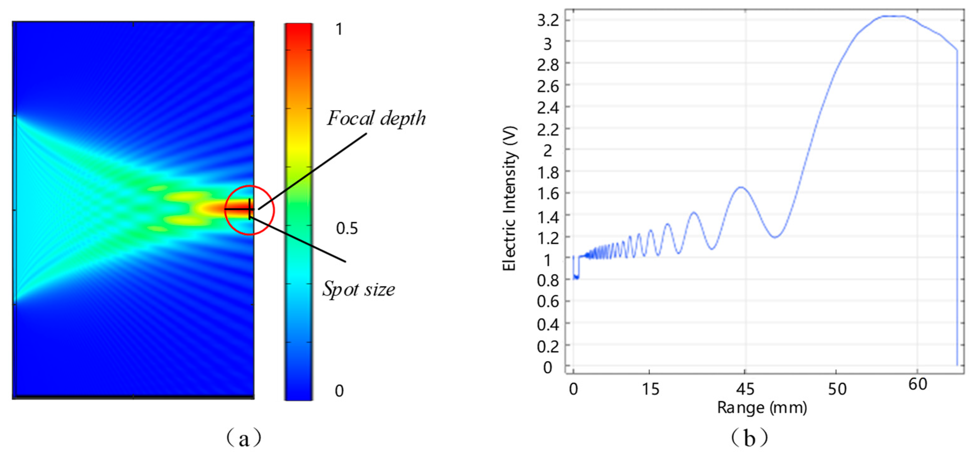
2.3.1. Cross-Range Resolution

In order to investigate the propagation model of continuous terahertz waves under a focusing lens, the finite element method is used for the simulation and modeling. Taking a lens with a focal length of 50 mm as an example, the lens has a diameter of 70 mm, a thickness of 10 mm, and a radius of curvature of 80 mm. The lens material is HDPE with a refractive index of 1.6. When the terahertz beam radiates from the horn antenna, it propagates outward in the form of fluctuations, which are Gaussian waves. However, under the action of a set of optical lenses, this beam is successively converted into a parallel beam and a focused beam. According to the Fresnel diffraction formula [35], the magnitude of the electric field at the exit side of the lens can be transformed into the focal plane, which is expressed as follows:

$$E\left(a,u\right)={\int }_{-\infty }^{\infty }E\left(x_0,y\right)\mathrm{e}\mathrm{x}\mathrm{p}\left(-i\pi y^2/\lambda a\right)\mathrm{e}\mathrm{x}\mathrm{p}\left(i2\pi uy/\lambda a\right)dy/\sqrt{a}f$$

(5)

where $\lambda$ is the wavelength, $a$ is the focal length, $u/\lambda a$ is called the spatial frequency, and $E\left(x_0,y\right)$ and $E\left(a,u\right)$ are the electric field amplitudes at the exit plane $x=x_0$ and at the focal plane $x=a$, respectively.

In general, it is very challenging to simulate systems with optical lenses using standard full vector wave analysis methods. In this simulation experiment, the focusing lens is analyzed using the “electromagnetic wave, frequency domain” interface and the “electromagnetic wave, beam envelope” interface. The former only analyzes the domain of the lens and its vicinity, where the boundary field at the exit surface of the lens is propagated to the focal plane using the Fresnel diffraction formula. The “transition” boundary condition is based on the assumption that the wave propagates in a direction perpendicular to the inner boundary of the thin antireflective coating. In particular, the wave propagates in a direction close to the normal direction. The analysis of the latter includes the entire domain of the focal plane and uses the same “transition” boundary conditions. This has the advantage that the thin antireflective coating does not need to be represented by a thin domain around the lens. Figure 3 shows the electromagnetic wave propagation model under a 50 mm focusing lens. As the beam passes through the lens, the simulation results demonstrate how the shape and refractive properties of the lens affect the behavior of the beam. The lens causes the parallel beams to change their direction of propagation and converge toward the focal point, forming a focused beam (Figure 3a). And there exists a focused spot with a diameter of about 2 mm at the focal position; this also determines the minimum defect size detected by the system. Figure 3b illustrates the variation in the energy curve on the centerline of the lens.

2.3.2. Range Resolution

According to Equation (3), the range resolution of the continuous terahertz detection system is limited by the transmission medium and the operating bandwidth. A Hanning window is often introduced in chirp signal processing to reduce the return echo side-lobe at the expense of widening the main lobe. However, this further reduces the resolution of the measurement. In this way, the range resolution can be expressed as follows:

$$\mathsf{\Delta }d=\alpha c/2nB$$

(6)

where $\alpha$ is the broadening factor. In a practical application, the minimum resolution also relates to the sampling rate and number of sampling points. Therefore, the measured minimum range resolution can be provided by the following formula:

$$\mathsf{\Delta }{d}_{\mathrm{r}\mathrm{e}\mathrm{a}\mathrm{l}}=\alpha c{t}_s{f}_s/2nBN$$

(7)

where $f_s$ is the system sampling rate, $N$ is the number of sampling points, and $f_s/N$ represents the minimum interval of the actual spectrum in the signal acquisition process. In practice, the number of sampling points cannot be infinitely long. Therefore, it is necessary to use the spectrum correction and refinement method to improve the accuracy of the thickness measurement.

3. Spectrum Correction and Refinement Method

In fact, the continuous terahertz detection system acts as a detector and needs to be combined with signal processing methods to achieve highly accurate measurements. A new spectrum correction and refinement signal processing method is proposed in this paper to address the problems of window truncation, spectrum leakage, and the picket fence effect.

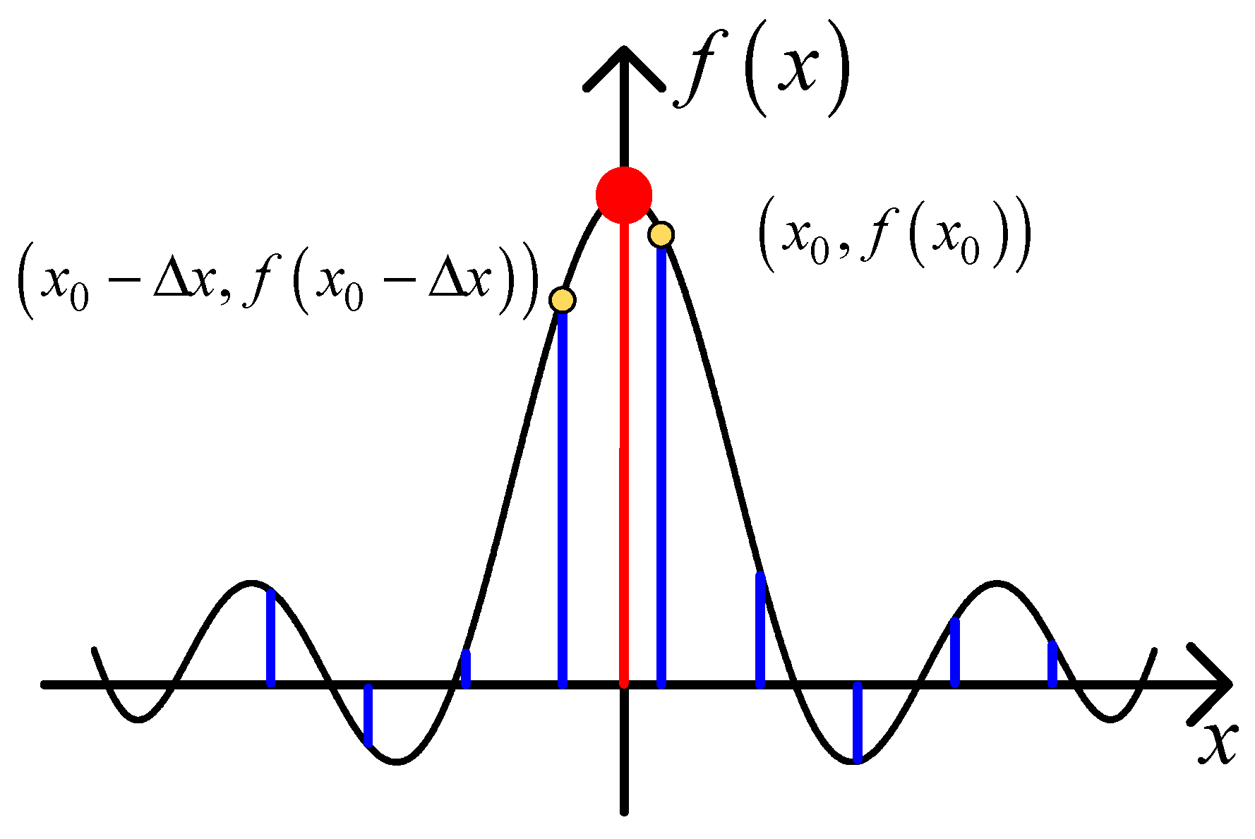
3.1. Frequency Correction Based on Ratio Method

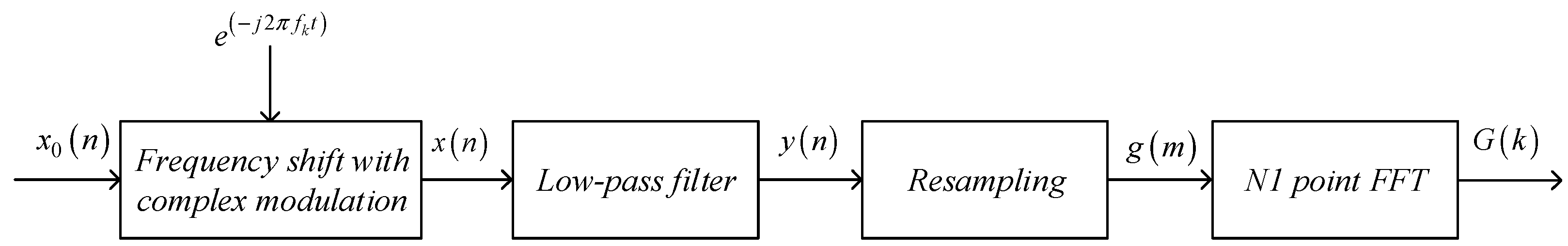
The ratio method of discrete spectral correction is a method of correcting and compensating for irregularities or aberrations in spectral measurements. The ratio method involves introducing a reference signal and a correlation signal of a known flat spectrum into the measurement system. The reference signal serves as a benchmark for comparison. The principle of the ratio method is to calculate the ratio of the measured spectrum to the reference spectrum at each frequency point. The ratio indicates the gain or attenuation introduced by the measurement system at a particular frequency. The measured spectrum is divided point-by-point with the reference spectrum, and the resulting ratio spectrum represents the frequency response of the system. Irregularities or deviations in the ratio spectrum indicate areas where the measurement system introduces errors or variations in the signal amplitude. For spectral correction, these irregularities need to be inverted and applied to the measured spectrum. The measured spectrum is multiplied by the inverse of the ratio spectrum to obtain the corrected spectrum. The common methods for solving the equation are the ratio formula method, iterative solution method, and peak search method. To simplify the calculation, the ratio formula method is used to directly derive the formula for calculation. In terahertz FMCW systems, the frequency of the differential beat signal reflects the distance information, while the phase is generally not analyzed. Therefore, this paper only describes the frequency solving process of the ratio method and does not analyze the phase solving process.

Figure 4 shows the spectral diagram of the window function, in which the highest and second-highest lines in the discrete blue line spectrum are located on both sides of the actual spectral peak. The amplitude ratio function of two adjacent spectral lines in the spectrum can be expressed by the following formula:

$$y=F\left(x\right)=f\left(x\right)/f(x+∆x)$$

(8)

where $f\left(x\right)$ is defined as the spectral function, $y=F\left(x\right)$ is the ratio function of $f\left(x\right)$ and $f(x+∆x)$, $∆x$ is the frequency interval, and the inverse function of the above equation can be obtained as follows:

$$x=g\left(y\right)$$

(9)

Then, the frequency correction is $∆x=∆k$. The corrected frequency is $\left(k+∆k\right)·f_s/N$, where $k (k=\mathrm{0,1},2,\cdots ,N⁄2-1)$ is the number of spectral lines, and $N$ is the number of sampling points.

As shown in Figure 4, the highest and second-highest spectral lines in the discrete blue spectral lines are located on both sides of the actual spectral peak, respectively, denoted as $\left(x_0,f\left(x_0\right)\right)$ and $\left(x_0+∆x,f\left(x_0+∆x\right)\right)$. For a single-frequency signal with frequency $k$, the principal flap function can be expressed as $y=Af\left(x-k\right)$. For the Hanning window function, it is assumed that the FFT of the signal is $N$ spectral lines, the maximum value is located at the $M$ th, and the frequency interval is $∆f$. The corrected frequency $f_c$ and amplitude $A_c$ can be expressed by the following equations:

$$f_c=(M+∆N)f_s/N$$

(10)

$$A_c=2\pi ∆N·\left(1-{∆k}^2\right)y_M/\mathrm{s}\mathrm{i}\mathrm{n}\left(\pi ∆k\right)$$

(11)

The ratio correction method is better for single-frequency signal correction, but less effective for multi-frequency signals. Particularly for thickness measurements of layered structures, multiple media layers with tiny thicknesses mean that there are multiple peaks in the signal spectrum. The spectrum refinement method provides a good solution, which is analyzed in detail below.

3.2. Zoom-FFT

In fact, the spacing between adjacent spectral lines—that is, the frequency resolution ($∆f=f_s/N$)—determines the resolution of the signal detection. The smaller $∆f$ is, the higher the resolution of the spectrum, and less useful information is lost due to the picket fence effect. When the sampling frequency $f_s$ is determined, $∆f$ is determined by the number of sampling points $N$, and the number of displayable spectral lines is $N/2$. In this system, the number of sampling points $N$ is 1024; therefore, the maximum number of spectral lines is 512. Considering the transition band effect of the analog anti-aliasing filter, the number of spectral lines is generally set to 400. To improve the frequency resolution without changing the upper limit frequency ($f_s/2$), the zero-padding method of increasing the window length is commonly adopted. However, this can easily lead to an increase in computational workload and complexity. In the case of a limited sampling length and computational memory, a method of complex modulation fine spectrum analysis is proposed for spectrum refinement, which takes into account both the computational complexity and upper limit frequency without sacrificing the performance.

The complex modulation fine spectrum analysis method, also known as the Zoom-FFT or ZFFT, is a band-selective frequency refinement analysis method [36]. Figure 5 shows the processing flow of Zoom-FFT. The analog signal $x\left(t\right)$ undergoes an anti-aliasing filter and A/D conversion to obtain the sample time sequence $x_0\left(n\right)$, the discrete Fourier transform of which can be represented by the following equation:

$$X_0\left(k\right)={\sum }_{n=0}^{N-1}{x}_0\left(n\right)W_N^{nk},\left(k=\mathrm{0,1},2,\cdots ,N-1\right)$$

(12)

where $W_N=e^{-j2\pi /N}$. The sampled time series $x_0\left(n\right)$ is complexly modulated and the frequency shift signal can be expressed by the following equation:

$$x\left(n\right)=x_0\left(n\right)·\mathrm{e}\mathrm{x}\mathrm{p}\left(-j2\pi n{f}_e/f_s\right)=x_0\left(n\right)·\mathrm{c}\mathrm{o}\mathrm{s}\left(2\pi n{L}_0/N\right)-j{x}_0\left(n\right)·\mathrm{s}\mathrm{i}\mathrm{n}\left(2\pi n{L}_0/N\right)$$

(13)

where $f_e=\left(f_1+f_2\right)/2$ is the center frequency of the target band, and $L_0=f_e/∆f$ is the frequency center shift. According to the discrete Fourier transform (DFT) frequency shift characteristic, the relationship between the discrete spectrum $X\left(k\right)$ of $x\left(n\right)$ and the discrete spectrum $X_0\left(k\right)$ can be expressed by the following equation:

$$X\left(k\right)=X_0\left(k+L_0\right),\left(k=\mathrm{0,1},2,\cdots ,N-1\right)$$

(14)

The resampling of the signal spectrum after complex modulation can be performed by reducing the sampling frequency to $f_s/D$, where $D$ is the scale factor, also known as the selected sampling ratio. To avoid mixing after resampling, a low-pass filter should also be introduced. The cut-off frequency of the low-pass filter is $f_s/2D$, and the output signal can be expressed by the following equation:

$$Y\left(k\right)=X\left(k\right)H\left(k\right)$$

(15)

where $H\left(k\right)$ is the frequency response of the low-pass filter. The output time domain signal can be expressed as follows:

$$y\left(n\right)={\sum }_{k=0}^{N-1}Y\left(k\right)W_N^{-nk}/N$$

(16)

Resampling $y\left(n\right)$ through a scale factor $D$ yields a new signal, which can be expressed as:

$$g\left(m\right)=y\left(Dm\right)$$

(17)

According to the DFT principle, the spectrum of $g\left(m\right)$ can be obtained by the following equation:

$$G(k)={\displaystyle {\sum }_{m=0}^{N-1}g(m)}{W}_N^{mk}=\left\{\begin{array}{cc}{x}_0(k+L_0)/D& (k=0,1,2,\cdots ,N/2-1)\\ x_0(k+L_0-N)/D& (k=N/2,N/2+1,\cdots ,N-1)\end{array}\right.$$

(18)

It can be seen that after the above conversion, the frequency resolution can be improved by a factor of $D$ compared to the direct FFT method. Commonly used spectrum analyzers use this algorithm for refinement analysis. However, the maximum refinement multiplier $D$ is limited by the characteristics of the low-pass filter. The Zoom-FFT eliminates the computation of narrow-band and out-of-band spectral lines, but the complex modulation and digital filtering still require a large amount of computation. In fact, the memory space needed to store the intermediate data limits the maximum refinement multiplier. When $D=1000$, then $1000\ast 1024\ast 2$ points of memory space are required to store the data. As the refinement multiplier increases, the transition band width has an increasing impact on the filtering accuracy, which can easily lead to the non-target frequency components not being effectively filtered out or the target frequency components being misjudged as noise. The complex modulation refinement spectrum method based on the complex analytic bandpass filter proposed in this paper only offsets the refinement selection sampling points, which takes into account the computational accuracy and efficiency.

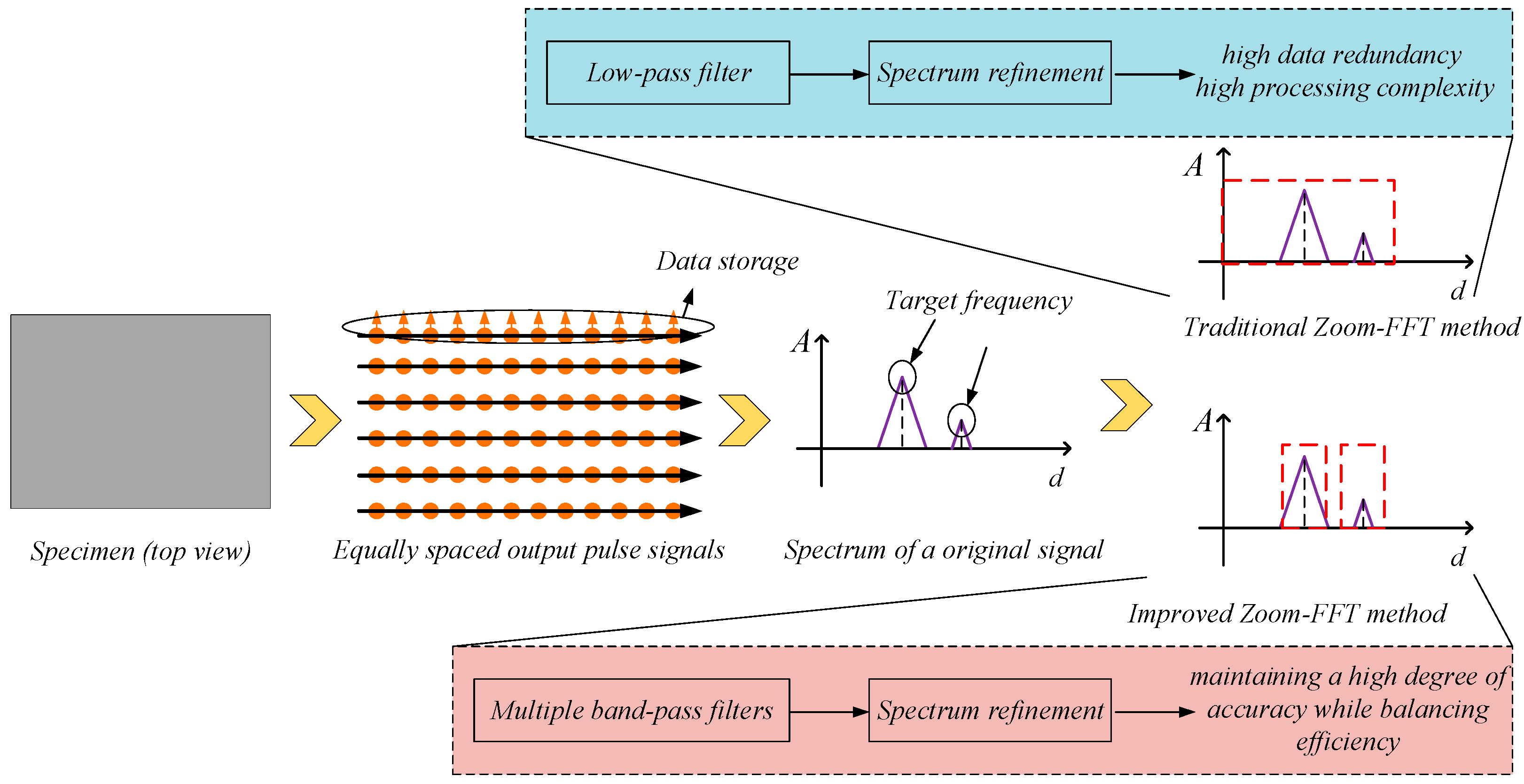
3.3. Improved Refinement Spectrum Method

By constructing a complex analytic bandpass filter, a faster computation speed and smaller storage space can be obtained, and the frequency aliasing caused by edge errors of low-pass antialiasing filters can be effectively avoided. This improved method increases the efficiency of its detection while maintaining its accuracy. Figure 6 demonstrates the principle and advantages of the improved spectrum refinement method. Multiple bandpass filters are constructed to reduce computational redundancy.

First, a real low-pass filter is constructed, for which the cutoff frequency and impulse response can be expressed by the following equations:

$${\omega }_0=\left({\omega }_2-{\omega }_1\right)/2$$

(19)

$$h_1\left(k\right)={\int }_{-{\omega }_0}^{{\omega }_0}{e}^{-j\omega k}d\omega /2\pi =\mathrm{s}\mathrm{i}\mathrm{n}\left(k{\omega }_0\right)/k\pi \left(k=0,\pm 1,\pm 2,\cdots \right)$$

(20)

where the bandwidth is ${\omega }_2-{\omega }_1$. Then, the low-pass filter is complexly shifted to make its congruence center move from $0$ to ${\omega }_c$. The impulse response of the new analytic filter can be represented by the following equation:

$$h^0\left(k\right)=h_1\left(k\right)e^{j{\omega }_{c}k}=h_1\left(k\right)\left[\mathrm{c}\mathrm{o}\mathrm{s}\left({\omega }_{c}k\right)+j\mathrm{s}\mathrm{i}\mathrm{n}\left({\omega }_{c}k\right)\right] \left(k=0,\pm 1,\pm 2,\cdots \right)$$

(21)

Obviously, $h^0$ is a complex function, meaning its real and imaginary parts can be represented as follows:

$$h_{\mathrm{R}}^0\left(k\right)=\left[\mathrm{s}\mathrm{i}\mathrm{n}\left({\omega }_{0}k\right)\mathrm{c}\mathrm{o}\mathrm{s}\left({\omega }_c\right)\right]/\pi k (k=0,\pm 1,\pm 2,\cdots )$$

(22)

$$h_{\mathrm{I}}^0\left(k\right)=\left[\mathrm{s}\mathrm{i}\mathrm{n}\left({\omega }_{0}k\right)\mathrm{s}\mathrm{i}\mathrm{n}\left({\omega }_c\right)\right]/\pi k (k=0,\pm 1,\pm 2,\cdots )$$

(23)

where ${\omega }_c=\left({\omega }_1+{\omega }_2\right)/2$. Finally, decimation filtering and frequency shifting are performed. Based on the above analysis, the processing flow of the improved continuous terahertz detection algorithm can be summarized as follows (Algorithm 1):

Algorithm 1: Improved Refinement Spectrum Method.

Input: the original sampled signal $x_0\left(n\right)$, refinement multiplier $D$, Target band $\left(f_1,f_2\right)$, Center frequency $f_c=\left(f_1+f_2\right)/2$, and then the sampling rate after decimation is $f_s/D$, and the analyzed frequency band can be represented as $\left[-f_s/2D,f_s/2D\right]$.

Step 1. Hanning window processes the original signal $x_0\left(n\right)$. Step 2. A real low-pass filter with cutoff frequency $f_s/2D$ is constructed, and the complex modulation shift with offset $2\pi f_c$ is performed to obtain a complex analytic band-pass filter with width $f_s/D$. Step 3. The original signal $x_0\left(n\right)$ is selectively sampled with a complex analytic bandpass filter to generate a complex analytic signal $\overline{x}\left(n\right)$ with a frequency in the range of $f_1$ to $f_2$, with the selective sampling ratio of D. Step 4. The signal $\overline{x}\left(n\right)$ is frequency shifted by complex modulation to shift the starting frequency of refinement to zero frequency point. $\overline{y}\left(n\right)=\overline{x}\left(n\right)s\left(n\right)$, where $s\left(n\right)=e^{-j{\omega }_{1}n}$ is multiple carrier signals, and ${\omega }_1=2\pi f_1/f_s$; the amount of complex modulation frequency shift is ${\overline{\omega }}_1={\omega }_{1}D$. Step 5. N-point FFT was conducted for $\overline{y}\left(n\right)$ and spectral analysis was performed.

Output: Spectrum with distinct independent dominant flaps.

4. Results

4.1. Cross-Range Test

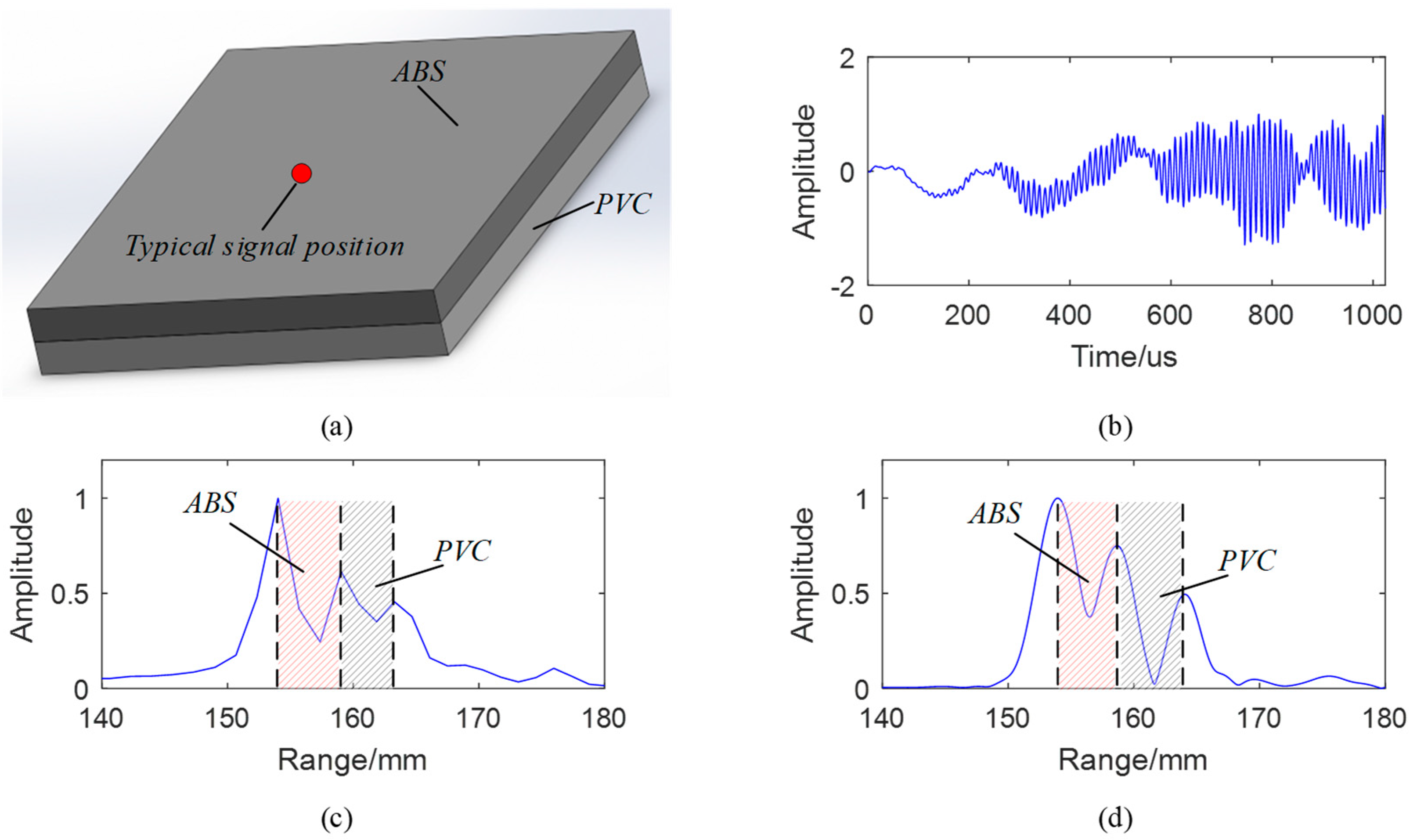
In this experiment, circular rings with different aperture diameters were fabricated using a 3D printer to verify the lateral resolution of the system under a 50 mm lens. The dimensional specifications and detection scheme of the sample are shown in Figure 6. The samples were placed on a metal plate, and the effect of the total reflection on the metal surface was utilized to quantitatively analyze the minimum resolving distance under the 50 mm lens. Figure 7 shows the test results. The minimum detectable diameter is about 2 mm, which is close to the theoretical value.

4.2. Range Test

4.2.1. Simulation

We used simulation software to generate a set of multi-frequency signals, which can be represented by the following formula:

$$x\left(t\right)=A_1\cos \left(2\pi f_{1}t\right)+A_2\cos \left(2\pi f_{2}t\right)+A_3\cos \left(2\pi f_{3}t\right)$$

(24)

The above equation is a generalized expression for the simulation experiment. When two of f₁, f₂, and f₃ are 0, this represents the measurement of the distance. When any two are not equal to 0, this represents the measurement of the single-layer thickness. When none of them are 0, this represents the measurement of the two-layer thickness.

In this experiment, the bandwidth $B$ is 56 GHz, the sweep time $t_s$ is 1.024 ms, the refractive index $n$ is 1, the sampling frequency $f_s$ is 1 MHz, the number of sampling points $N$ is 1024, and the refinement multiplier $D$ is 50. Therefore, the frequency resolution $∆f$ is 976.56 Hz. According to Equation (3), assuming that the targets to be detected are located at 50 mm, 60 mm, and 63 mm, respectively, the frequencies $f_1~f_3$ are 18,229 Hz, 21,875 Hz, and 22,969 Hz. By adding a Hanning window function and FFT transformation, the panoramic spectrum can be obtained. As the differences in the frequencies corresponding to these targets satisfy the frequency resolution condition, the ratio method can be used for correction.

Table 2. Results of different signal processing methods (frequency deviation).

	Distance Measurement			Thickness Measurement
				Single Layer		Two Layers
				Spectral Peak 1	Spectral Peak 2	Spectral Peak 1	Spectral Peak 2	Spectral Peak 3
Range (mm)	50	60	63	50	60	50	60	63
Theoretical frequency (Hz)	18,229	21,875	22,969	18,229	21,875	18,229	21,875	22,969
FFT	−321	395	−471	−321	395	−321	395	−471
Zero-padding	−31	−25	−21	29	−55	29	115	−881
Ratio method	0	0	0	−7	7	−8	−241	25
Energy centrobaric method	−9	15	−25	−6	12	−5	297	−138
FFT + FT	−16	−10	−6	19	−55	49	55	−211
CZT	−11	−5	−1	19	−55	49	55	−211
Proposed method	−1	5	−1	19	−50	42	49	−181

presents the results of direct FFT transformation, the zero-padding method, the ratio method, the energy centrobaric method, FFT + FT, CZT, and the proposed method. Frequency deviation is defined as the difference between the frequency calculated by each method and the theoretical frequency. The deviations in the frequency in the table are related to the theoretical values, where a positive deviation means that the frequency value is greater than the theoretical value and a negative deviation means that the frequency value is less than the theoretical value. The computational complexity is outlined in

Table 3. Computational complexity of different signal processing methods.

Methods	Computational Complexity
Ratio method	$\mathrm{O}\left(N\right)$
Energy centrobaric method	$\mathrm{O}\left(NlogN\right)$
FFT + FT	$\mathrm{O}\left(NlogN+N^2\right)$
CZT	$\mathrm{O}\left(NlogN+MlogM+N\times M\right)$
Proposed method	$\mathrm{O}\left(D\ast NlogN\right)$

, where $N$ is the signal length and $M$ is the number of sampling points.

Combining the experimental principles and simulation results, it can be seen that for the correction of single-frequency signals (distance measurement), the ratio method is superior in terms of the accuracy and computational complexity. The energy centrobaric method performs spectral correction by calculating the energy center of gravity of the spectrum, which has a relatively high computational complexity and reduced accuracy. For the correction of multi-frequency signals (thickness measurement), both the energy centrobaric method and ratio method have large errors. The FFT + FT method requires Fourier interpolation, and the CZT method requires the introduction of a chirp signal to replace the complex exponential function for non-uniform frequency sampling and a high-resolution estimation. Therefore, the FFT + FT and CZT methods are computationally intensive and are not applicable to engineering practice. The method proposed in this paper can balance the computational accuracy and efficiency and can effectively deal with the dense frequency analysis problem.

4.2.2. System Test

To test the actual detection capability of the proposed system, thickness measurement experiments were conducted on specimens bonded to ABS and PVC plates ($n_{ABS}=1.6$, and $n_{PVC}=1.9$ in the range of 126 GHz~182 GHz). The specimen structure and detection results are shown in Figure 8. The real thickness of the ABS and PVC are 5.10 mm and 5.13 mm, respectively.

As shown in Figure 8b,c, the original signals collected by the system are time-domain signals, which can be characterized after the filtering of the Hanning window and FFT transformation. Figure 8d shows the calculation results of a typical spectrum refinement method (zero-padding), and the calculation results of the other methods are outlined in

Table 4. Measurement results of different signal processing methods.

Methods	ABS			PVC
	Real Thickness (mm)	Measured Thickness (mm)	Error (%)	Real Thickness (mm)	Measured Thickness (mm)	Error (%)
FFT	5.10	4.94	3.14	5.13	4.16	18.91
Zero-padding	5.10	4.80	5.88	5.13	5.4	5.26
Ratio method	5.10	4.74	7.06	5.13	5.39	5.07
energy centrobaric method	5.10	4.72	7.45	5.13	5.20	1.37
FFT + FT	5.10	5.45	6.86	5.13	4.32	15.79
CZT	5.10	4.81	5.69	5.13	4.32	15.79
proposed method	5.10	4.98	2.35	5.13	5.21	1.56

. The actual detection capability is improved by the other calibration algorithms. The spectral refinement method proposed in this paper balances detection efficiency and accuracy, and it has high applicability, but the steps are more cumbersome. The appropriate signal processing method should be selected according to the actual demand in engineering applications. In addition, there is still a deviation between the measured results and the actual measured values, which may be caused by the Fabry–Perot effect. Future research should focus on using a continuous terahertz propagation model in the layered structure to correct the final results.

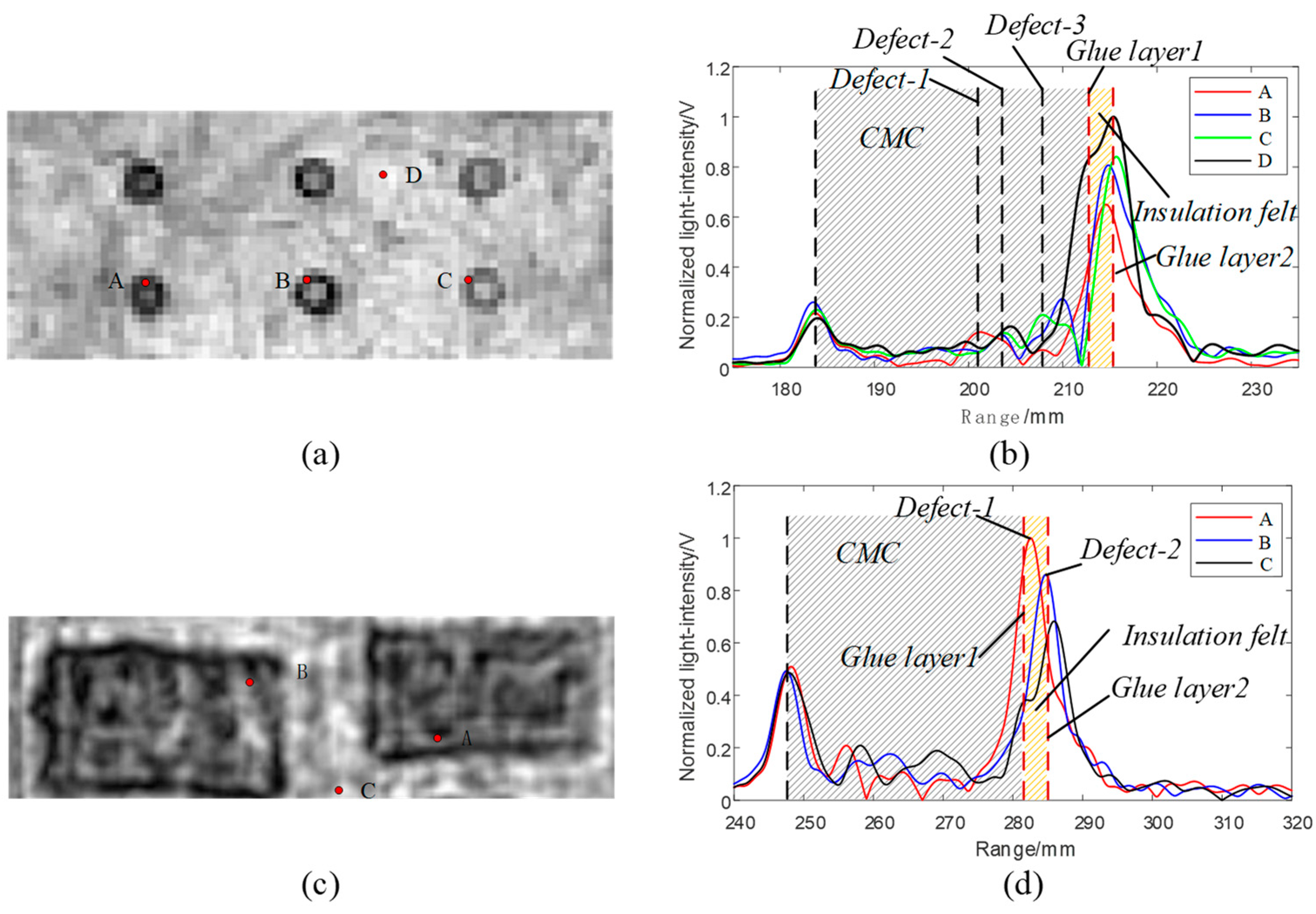
4.2.3. Application of Terahertz Detection in Ceramic Matrix Composites

Ceramic matrix composites (CMCs), as an important part of the thermal protection structure (TPS), have been widely used in reusable spacecrafts due to their light weight, high-temperature resistance, and high hardness. The TPS is composed of CMCs, insulation felt, and a protected structure. However, due to the harsh service environment, the TPS is prone to defects such as debonding, delamination, or ceramic pores, which have potential safety hazards. In this study, two TPS samples were prepared with pre-designed internal defects. Sample 1 has three rows of pore defects with different depths of a 5 mm diameter embedded in the ceramic layer at distances of 19 mm, 21 mm, and 24 mm from the surface, respectively. Sample 2 has pre-designed debonding defects in different adhesive layers. The basic structures of Sample 1 and Sample 2 are shown in Figure 9, and the detection results and typical signal schemes are shown in Figure 10. In this experiment, a 50 mm lens was used, and the surface of the CMCs was set as the focusing plane, with a step size of 1 mm.

Figure 10a shows the scanning imaging results of Sample 1, which clearly reveal the pore defects in the ceramic layer. Figure 10b provides typical signal schemes of the pore defects of different depths, and analysis of the data indicates that the distances from the surface are 19.50 mm, 21.60 mm, and 24.10 mm, respectively. Figure 10c shows the scanning imaging results of Sample 2. Figure 10d provides typical signal schemes for different debonding layers. It is worth noting that in the distance dimension, the signal at the no-defect position (black line) has two peaks at around 285 mm, corresponding to glue layer 1 and glue layer 2, respectively. Thus, the debonding layer can be determined based on characteristic signal analysis. These findings provide new detection ideas and methods for the NDT of layered structures.

5. Conclusions

Continuous terahertz scanning imaging has a large application prospect in the field of NDT in industry due to its advanced device integration and high output power. This paper presents a continuous terahertz detection system with a central frequency of 154 GHz and a bandwidth of 56 GHz. An improved spectral refinement method is proposed for the measurement of the calibration, which constructs a complex analytic bandpass filter to improve the computational speed and reduce frequency aliasing. Several frequency calibration methods are analyzed through the use of simulation and experimental tests, and a method that balances measurement accuracy and efficiency is proposed. In addition, research into the detection of the layered TPS is conducted. The experimental results indicate that the proposed system and detection method provide new ideas for the detection and location of internal defects in layered structures. However, due to the effects of spectral scattering and the aperture size of the focused lens, the quantitative analysis of the defects still requires further exploration.

References

1. Ellrich, F.; Bauer, M.; Schreiner, N.; Keil, A.; Molter, D. Terahertz Quality Inspection for Automotive and Aviation Industries. J. Infrared Millim. Terahertz Waves 2020, 41, 470–489. [Google Scholar] [CrossRef]
2. Akyildiz, I.; Jornet, J.; Chong, H. Terahertz band: Next frontier for wireless communications. Phys. Commun. 2014, 12, 16–32. [Google Scholar] [CrossRef]
3. Pawar, A.; Sonawane, D.; Erande, K.; Derle, D. Terahertz technology and its applications. Drug Invent. Today 2013, 5, 157–163. [Google Scholar] [CrossRef]
4. Kemp, M. Detecting hidden objects: Security imaging using millimetre-waves and terahertz. In Proceedings of the Conference on Advanced Video and Signal Based Surveillance, London, UK, 5–7 September 2007; pp. 7–9. [Google Scholar]
5. Oh, S.; Huh, Y.; Suh, J.; Choi, J.; Haam, S.; Son, J. Cancer diagnosis by terahertz molecular imaging technique. J. Infrared Millim. Terahertz Waves 2012, 33, 74–81. [Google Scholar] [CrossRef]
6. Zhang, X.; Guo, Q.; Chang, T.; Cui, H. Broadband stepped frequency modulated continuous terahertz wave tomography for nondestructive inspection of polymer materials. Polym. Test. 2019, 76, 455–463. [Google Scholar] [CrossRef]
7. Rubio-Cidre, G.; Badolato, A.; Ubeda-Medina, L.; Grajal, J.; Mencia, B.; Dorta-Naranjo, B. DDS-based signal-generation architecture comparison for an imaging radar at 300 GHz. IEEE Trans. Instrum. Meas. 2015, 64, 3085–3098. [Google Scholar] [CrossRef]
8. Kimmitt, M. Restrahlen to T-rays—100 years of terahertz radiation. J. Biol. Phys. 2003, 29, 77–85. [Google Scholar] [CrossRef]
9. Meta, A.; Hoogeboom, P.; Ligthart, L. Signal Processing for FMCW SAR. IEEE Trans. Geosci. Remote Sens. 2007, 45, 3519–3532. [Google Scholar] [CrossRef]
10. Gao, J.; Qin, Y.; Deng, B.; Wang, H.; Li, X. A novel method for 3-D millimeter-wave holographic reconstruction based on frequency interferometry techniques. IEEE Trans. Microw. Theory Tech. 2018, 66, 1579–1596. [Google Scholar] [CrossRef]
11. Sengupta, K.; Nagatsuma, T.; Mittleman, D. Terahertz integrated electronic and hybrid electronic–photonic systems. Nat. Electron. 2018, 1, 622–635. [Google Scholar] [CrossRef]
12. Ako, R.; Upadhyay, A.; Withayachumnankul, W.; Bhaskaran, M.; Sriram, S. Dielectrics for Terahertz Metasurfaces: Material Selection and Fabrication Techniques. Adv. Opt. Mater. 2020, 8, 1900750. [Google Scholar] [CrossRef]
13. Yang, Y.; Yamagami, Y.; Yu, X.; Pitchappa, P.; Webber, J.; Zhang, B.; Fujita, M.; Nagatsuma, T.; Singh, R. Terahertz topological photonics for on-chip communication. Nat. Photonics 2020, 14, 446–451. [Google Scholar] [CrossRef]
14. Alsharif, M.H. Activities, Challenges and Potential Solutions. Symmetry 2020, 12, 676. [Google Scholar] [CrossRef]
15. Cooper, K.B.; Dengler, R.J.; Llombart, N.; Thomas, B.; Siegel, P.H. THz Imaging Radar for Standoff Personnel Screening. IEEE Trans. Terahertz Sci. Technol. 2011, 1, 169–182. [Google Scholar] [CrossRef]
16. Stantchev, R.I.; Yu, X.; Blu, T.; Pickwell-MacPherson, E. Real-time terahertz imaging with a single-pixel detector. Nat. Commun. 2020, 11, 2535–2538. [Google Scholar] [CrossRef]
17. Federici, J.F.; Schulkin, B.; Huang, F.; Gary, D.; Barat, R.; Oliveira, F.; Zimdars, D. THz imaging and sensing for security applications—Explosives, weapons and drugs. Semicond. Sci. Technol. 2005, 20, S266–S280. [Google Scholar] [CrossRef]
18. Yu, C.; Fan, S.; Sun, Y.; Pickwell-MacPherson, E. The potential of terahertz imaging for cancer diagnosis: A review of investigations to date. Quant. Imaging Med. Surg. 2012, 2, 33. [Google Scholar]
19. Schreiner, N.S.; Sauer-Greff, W.; Urbansky, R.; Freymann, G.V.; Friederich, F. Multilayer Thickness Measurements below the Rayleigh Limit Using FMCW Millimeter and Terahertz Waves. Sensors 2019, 19, 3910. [Google Scholar] [CrossRef]
20. Cristofani, E.; Friederich, F.; Wohnsiedler, S.; Matheis, C.; Beigang, R. Non-Destructive Testing Potential Evaluation of a THz Frequency-Modulated Continuous-Wave Imager for Composite Materials Inspection. Opt. Eng. 2014, 53, 031211. [Google Scholar] [CrossRef]
21. Xue, K.; Chen, Y.; Zhang, W.; Song, J.; Wang, Z.; Jin, Y.; Guo, X. Continuous Terahertz Wave Imaging for Debonding Detection and Visualization Analysis in Layered Structures. IEEE Access 2023, 11, 31607–31618. [Google Scholar] [CrossRef]
22. Giovannacci, D.; Cheung, H.; Walker, G.C.; Bowen, J.W.; Martos-Levif, D.; Brissaud, D.; Cristofol, L.; Mélinge, Y. Timedomain imaging system in the terahertz range for immovable cultural heritage materials. Strain 2019, 55, e12292. [Google Scholar] [CrossRef]
23. Huang, H.; Qiu, P.; Panezai, S.; Hao, S.; Zhang, D.; Yang, Y.; Ma, Y.; Gao, H.; Gao, L.; Zhang, Z.; et al. Continuous-wave terahertz high-resolution imaging via synthetic hologram extrapolation method using pyroelectric detector. Opt. Laser Technol. 2019, 120, 105683. [Google Scholar] [CrossRef]
24. Wang, Q.; Zhang, X.; Xu, Y.; Gu, J.; Li, Y.; Tian, Z.; Singh, R.; Zhang, S.; Han, J.; Zhang, W. Broadband metasurface holograms: Toward complete phase and amplitude engineering. Sci. Rep. 2016, 6, 32867. [Google Scholar] [CrossRef] [PubMed]
25. Niu, T.; Withayachumnankul, W.; Upadhyay, A.; Gutruf, P.; Abbott, D.; Bhaskaran, M.; Sriram, S.; Fumeaux, C. Terahertz reflectarray as a polarizing beam splitter. Opt. Express 2014, 22, 16148–16160. [Google Scholar] [CrossRef] [PubMed]
26. Zhang, T.; Huang, H.; Zhang, Z.; Gao, H.; Gao, L.; Zheng, Z. Sensitive characterizations of polyvinyl chloride using terahertz time-domain spectroscopy. Infrared Phys. Technol. 2021, 118, 103878. [Google Scholar] [CrossRef]
27. Liu, H.; Zhang, Z.; Zhang, X.; Yang, Y.; Zhang, Z.; Liu, X.; Wang, F.; Han, Y.; Zhang, C. Dimensionality reduction for identification of hepatic tumor samples based on terahertz time-domain spectroscopy. IEEE Trans. Terahertz Sci. Technol. 2018, 8, 271–277. [Google Scholar] [CrossRef]
28. Zhang, X.; Chang, T.; Wang, Z.; Cui, H. Three-dimensional terahertz continuous wave imaging radar for nondestructive testing. IEEE Access 2020, 8, 144259–144276. [Google Scholar] [CrossRef]
29. Chen, H.M.; Lee, S.; Rao, R.M.; Slamani, M.-A.; Varshney, P.K. Imaging for concealed weapon detection: A tutorial overview of development in imaging sensors and processing. IEEE Signal Process. 2005, 22, 52–61. [Google Scholar] [CrossRef]
30. Sheen, D.M.; Hall, T.E.; Severtsen, R.H.; McMakin, D.L.; Hatchell, B.K.; Valdez, P.L.J. Standoff concealed weapon detection using a 350 GHz radar imaging system. In Proceedings of the Passive Millimeter-Wave Imaging Technology XIII, Orlando, FL, USA, 5–9 April 2009. [Google Scholar]
31. Essen, H.; Wahlen, A.; Sommer, R.; Konrad, G.; Schlechtweg, M. A Tessmann. Very high bandwidth millimetre-wave radar. Electron. Lett. 2005, 41, 1247–1249. [Google Scholar] [CrossRef]
32. You, C.; Lu, C.; Wang, T.; Qian, S.; Yang, Z.; Wang, K.; Liu, J.; Wang, S. Method for defect contour extraction in terahertz non-destructive testing conducted with a raster-scan THz imaging system. Appl. Opt. 2018, 57, 4884–4889. [Google Scholar] [CrossRef]
33. Bigman, D.P.; Day, D.J. Ground penetrating radar inspection of a large concrete spillway: A case-study using SFCW GPR at a hydroelectric dam. Case Stud. Constr. Mater. 2022, 16, e00975. [Google Scholar] [CrossRef]
34. Xu, L.; Lien, J.; Li, J. Doppler–Range Processing for Enhanced High-Speed Moving Target Detection Using LFMCW Automotive Radar. IEEE Trans. Aerosp. Electron. Syst. 2021, 58, 568–580. [Google Scholar] [CrossRef]
35. Cai, X.; Zheng, Y.; Zhu, Y. Convergence and divergence focusing phenomena at the focal plane of ultrashort pulses. J. Opt. Soc. Am. A 2020, 37, 969–973. [Google Scholar] [CrossRef] [PubMed]
36. Tang, B.; Zhang, J.; Hu, S.; Zhang, H.; Ge, G.; Qiu, K. Low Complexity Two-Stage FOE Using Modified Zoom-FFT for Coherent Optical M-QAM Systems. IEEE Photon. Technol. Lett. 2020, 32, 263–266. [Google Scholar] [CrossRef]
Figure 1. The principle of LFMCW measurement.
Photonics 10 01020 g001
Figure 2. Continuous terahertz scanning imaging scheme. (a) The architecture of the terahertz imaging system. (b) Full matrix sampling process diagram. (c) The workflow of the terahertz sensor.
Photonics 10 01020 g002
Figure 3. The electromagnetic wave propagation model under a 50 mm focusing lens. (a) Schematic of the simulation results. (b) Change in the energy curve on the lens centerline.
Photonics 10 01020 g003
Figure 4. Window function spectrum diagram.
Photonics 10 01020 g004
Figure 5. Window function spectrum diagram.
Photonics 10 01020 g005
Figure 6. The principle and advantages of the improved spectrum refinement method.
Photonics 10 01020 g006
Figure 7. Cross-range test schematic. (a) Specimen structure. (b) System detection scheme. (c) Scanning image.
Photonics 10 01020 g007
Figure 8. The specimen structure and detection results. (a) Structural scheme. (b) Original signal of typical location. (c) The Spectrum of window function change and FFT. (d) The result of typical spectrum refinement method (zero-padding).
Photonics 10 01020 g008
Figure 9. Structure of Sample 1 and Sample 2. Order of thickness in each layer is 29 mm (35 mm in sample 2), 0.2 mm/2 mm/0.2 mm/10 mm from top to bottom. (a) Sample 1 with the hole defects in the CMCs, which were in three rows of different depths. (b) Sample 2 with the debonding region in glue layer 1 and glue layer 2, respectively.
Photonics 10 01020 g009
Figure 10. Terahertz test results for Sample 1 and Sample 2. (a) Scanning image of Sample 1. (b) Typical signals of different positions, where A–D represents the signals of defect-1, defect-2, defect-3, and no-defect, respectively. (c) Scanning image of Sample 2. (d) Typical signals of different positions, where A–C represents the signals of defect-1, defect-2, and no-defect, respectively.
Photonics 10 01020 g010