Mirror Vibration Tolerance Studies in X-ray Free-Electron Laser Oscillator

Abstract

The X-ray free-electron laser oscillator (XFELO) has received significant attention due to its ability to produce fully coherent, high-brightness, and highly stable X-ray beams. Despite these advantages, the operation of the XFELO can be impeded by the surrounding environment. Specifically, vibrations of the optical components within the cavity can lead to poor alignment, which can diminish the interaction between the light and electrons in the undulator. Consequently, the quality of the output X-rays may be compromised. This study aims to investigate the impact of mirror vibrations on the output laser at various vibration frequencies. Firstly, we develop three single-frequency vibration models at 10 Hz, 0.01 MHz, and 1.1 MHz to investigate the changes in energy, spectral width, beam size, and beam divergence angle of the output laser. Secondly, we build a more complex multi-frequency vibration model based on the single-frequency one to simulate the realistic vibration of the mirror. Finally, we utilize the multi-frequency vibration model to investigate the tolerance limits of the output laser to vibration amplitude at different vibration frequencies of the mirror. The results show that the tolerance of the amplitude near the low and middle frequencies has less effect on the output power, which is approximately 250 nrad or more. However, in certain particular instances, particularly in the vicinity of the resonant frequency, there will be deviations from the tolerance limit. These deviations can result in values that are excessively high or excessively low. The study could prove useful in the future installation of XFELOs.

1. Introduction

Since the development of the X-ray free-electron laser, it has received wide attention and been used in applications in the fields of physics, biology, chemistry, and medicine due to its advantages of short wavelength, high energy, and good coherence [1,2,3,4]. During the development of the FEL, most of the operating modes were based on self-amplified spontaneous emission (SASE) [5,6,7], but the longitudinal coherence of SASE was suboptimal, so later researchers proposed X-ray free-electron laser oscillators (XFELOs) [8,9,10,11]. The XFELO stands out for its ability to generate a highly stable X-ray beam with high average brightness [12,13,14]. The XFELO setup generally comprises three key components: the crystal mirrors, the undulator, and the focusing elements [15,16,17,18]. The function of crystal mirrors is to ensure that the optical field forms a closed loop in the resonant cavity [19,20]. To achieve energy gains within this closed loop, the radiation field is directed through an undulator consisting of periodic magnet arrangements. Additionally, the inclusion of focusing elements is crucial to ensure the lateral stability of the radiation field throughout multiple round trips. When these three optical components are precisely aligned with each other, the saturated laser output remains stable and continuous. However, during actual operation, vibration of the optical components is always present due to external environmental factors.

Previous studies on alignment errors in optical cavities have primarily concentrated on investigating the impact of different deviations in the radian of the optical device on the output laser [21,22]. However, these studies have not provided an overall trend regarding the variation of the output laser with different vibration frequencies, nor have they investigated the severity of the effect induced by different vibration frequencies on the output laser. Therefore, this paper will commence by investigating the vibrations of mirrors and establishing a vibration model to simulate their motion. The objective is to study the effects of different vibration frequencies of the mirror on the output laser.

The structure of this article is as follows: Section 2 will introduce the parameters used in the numerical simulations and the design of the cavity structure. In Section 3, this study employs single-frequency vibration models and multi-frequency vibration models that have been built to conduct simulations. Then, a realistic set of measurement data is simulated and the results of this simulation are compared with the previous results. In Section 4, the multi-frequency vibration model is employed to investigate the amplitude tolerance limits of the output laser under varying vibration frequencies of the refractors. Furthermore, the relationship between the maximum amplitude and frequency is plotted and subjected to analysis. Section 5 concludes and analyses all the simulation results.

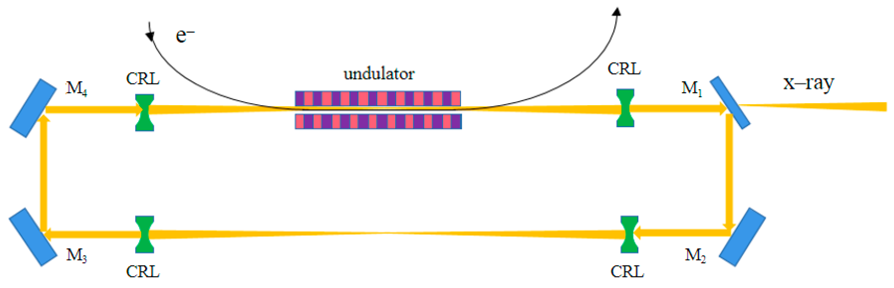
2. The Cavity Design and Parameters

The configuration of the cavity structure employed in this study to investigate the impact of crystal mirror vibration on light pulses is illustrated in Figure 1. It comprises three components: the undulator, the crystal mirror, and the focusing elements. The undulator consists of a series of magnets arranged periodically, spanning a total length of 12 m with a period length of 0.026 m. Electrons undergo a periodic twisting motion within the magnetic field and propagate longitudinally at a velocity approaching the speed of light, serving as the gain medium for radiation field amplification. The optical resonant cavity is composed of four diamond crystal mirrors $M_1,M_2,M_3,\mathrm{a}\mathrm{n}\mathrm{d} M_4$ and the focusing elements, the CRLs. To minimize energy loss during reflection, $M_2,M_3$, and $M_4$ are thick crystals with near total reflectivity, while $M_1$ is a thin crystal with a peak reflectivity of 90%, primarily employed for laser coupling output. The CRL elements are used to ensure effective transverse focusing of the laser during multiple round trips within the optical cavity [23].

The reference accelerator utilized in this study is SHINE’s superconducting linear accelerator, which provides an electron beam repetitive frequency at 1 MHz. To accommodate this frequency, the optical cavity structure has been meticulously designed to enable light to traverse a distance of 300 m during a single round trip within the cavity. From Figure 1, it can be seen that the distance from the undulator exit to the nearest CRL is 43.5 m, followed by a 22.5 m span between this CRL and $M_1$, with an additional 5 m separation between $M_1$ and $M_2$. Similarly, the spatial relationships among the undulator entrance, CRL, $M_4$, and $M_3$ remain consistent with their previous values. Since the resonant cavity is rectangular, the distances between the upper and lower components are the same. The focal length of all four CRLs is 55.7 m.

A range of parameters employed to study the effect of deflection of the optical devices on the output optical pulse are shown in

Table 1. Main parameters of the XFELO simulation for SHINE.

Parameter	Value
Electron energy (GeV)	8
Relative energy spread (%)	0.01
Repetition rate (MHz)	1
Peak current (A)	600
Normalized emittance (mm mrad)	0.4
Undulator period length (mm)	26
Light wavelength (nm)	0.096

. The majority of these parameters were sourced from SHINE, which is equipped with a superconducting linear accelerator that can offer high-quality electrons with an energy of 8 GeV, a peak current intensity of 600 A, and a repetitive rate of 1 MHz [24,25].

3. Simulation of Mirror Vibration

The numerical simulation of the XFELO is divided into three parts: the first part simulates the interaction between the radiation field and the electron beam in the undulator, which can be performed with the open-source Software GENESIS [26]. The second part simulates the transmission of X-rays in a vacuum. It can be performed with the 3D optical transmission software Optical Propagation Code (OPC) [27]. The diffraction of the 3D Bragg is performed by Bright, which was developed according to the theory of dynamical diffraction [28]. By exploiting the interconnection of these three software programs, we were able to complete the 3D numerical simulation of the XFELO.

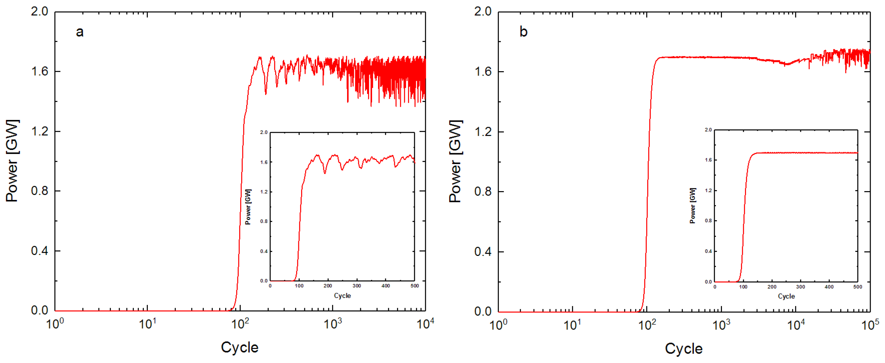
3.1. Perfect Alignment Cavity

Prior to conducting the simulations, it is essential to perform a perfect alignment simulation, which serves as a reference for subsequent analyses. Note that there are two kinds of XFELO simulation: time-independent simulation and time-dependent simulation. While the former provides faster calculations, but loses spectral information. In this simulation, the time-dependent simulation is chosen to ensure accuracy. However, it should be noted that when dealing with extensive calculations, employing the time-dependent simulation would require over a year to accomplish our goal. Therefore, in the subsequent simulations, we will employ the time-independent approach instead, which will be explained when it is used. Considering the substantial time requirement for time-dependent simulations, we have implemented measures to optimize efficiency. Specifically, the simulation utilizes 1001 electron beam slices and 450 round-trips. The simulation results are shown in Figure 2.

From Figure 2a, it can be seen that in the ideal situation of the first 100 oscillations, the light pulse energy has a very low value. However, as the oscillations progress from 100 to 180, the pulse energy increases rapidly until it reaches saturation. At this point, the pulse energy stabilizes at approximately 250 μJ. The spectrum of the optical pulse is shown in Figure 2b. It has a spectral bandwidth of 14.80 meV and good coherence. The size and divergence angle of the optical pulse are shown in Figure 2c,d. When the laser reaches saturation, the size and divergence angle remain at 45.35 μm and 0.34 μrad, respectively, similarly to the saturation energy, and do not change significantly.

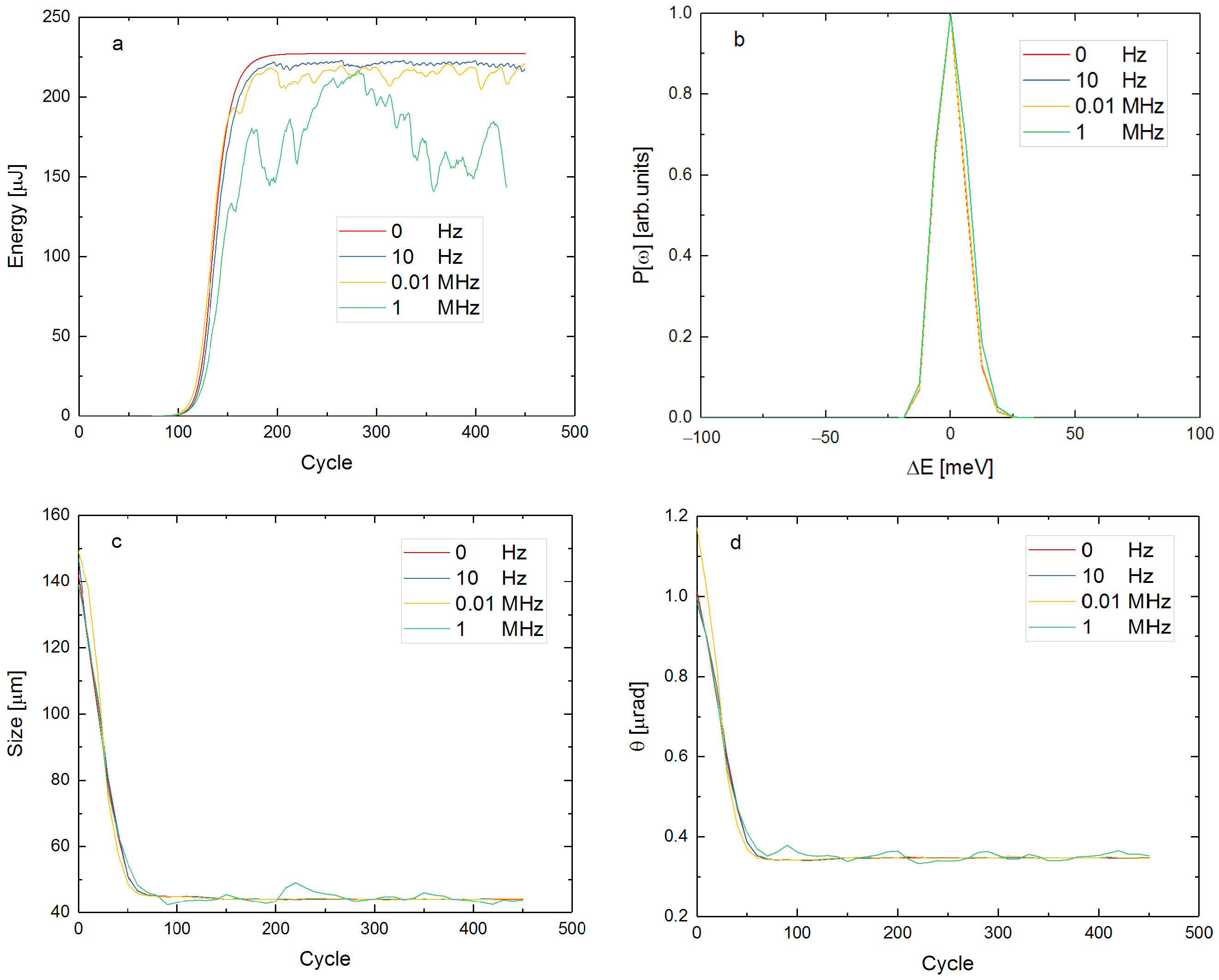
3.2. Single Frequency Vibration

A simplified vibration model was initially constructed, incorporating low, medium, and high frequencies as the vibration frequencies for the mirror. Specifically, the frequencies chosen were 10 Hz, 0.01 MHz, and 1.1 MHz, representing low, medium, and high frequencies, respectively. Their respective initial phases are chosen randomly in the range −π–π. Note that in the article, the four mirrors vibrate independently. The CRL elements do not vibrate and they are considered fixed. The resonant frequency of the mirror vibration and resonant cavity is 1 MHz. In order to avoid causing static misalignment in the single-frequency simulation results, 1.1 MHz is set as the high frequency. Furthermore, the low frequency of 10 Hz was determined from a set of realistic measured data. By analyzing these data, a time and frequency domain plot of the vibration can be derived, as shown in Figure 3.

The amplitude of the vibration is approximately 50 nrad as can be seen in Figure 3a, and the frequency of the vibration is concentrated around 100 Hz as shown in Figure 3b; therefore, the low frequency is set to 10 Hz, and the amplitude of the three single-frequency vibration models is also set to 50 nrad according to the time domain plot in Figure 3a. After the parameters have been set, the three single-frequency vibration models are simulated by incorporating the vibration of sinusoidal mode to obtain the results shown in Figure 4.

From Figure 4a, it can be seen that the saturation energy of the laser has decreased significantly compared to the ideal conditions at 10 Hz, 0.01 MHz, and 1.1 MHz vibration, fluctuating around 200 μJ, but the energy fluctuations do not change significantly with increasing frequency if only compared at these three frequencies. As can be seen in Figure 4b–d, the vibration of the mirror has little effect on the spectrum, beam size, and beam divergence angle of the output light (the spectral bandwidths at the three vibration frequencies are 14.90 meV, 14.94 meV, and 14.91 meV. The beam size and beam divergence angle have small fluctuations around 45.35 μm and 0.34 μrad, respectively). Note that since the spectra were normalized with the maximum of each simulation separately, Figure 4b has the same peaks. Figure 6b is the same for the same reason.

There are two anomalies, one of which is that when the vibration frequency of the mirror increases, the effect on the output light should theoretically increase. However, in three single-frequency simulations, the expected result did not occur; instead, the saturation energy at 1.1 MHz fluctuated in a range less than 0.01 MHz. The reason for this is speculated to be that 1.1 MHz is near the resonant frequency. Although the existence of static deviation is avoided, there is a high probability that the amplitude of the mirror is at a lower value when the light interacts with the mirror. Therefore, the effect on the output laser is small. When the vibration of the mirror is simulated using multiple frequencies, the results should be very different from the current results. This will be confirmed in the multi-frequency simulations below. Another anomaly arises when the mirror vibrates at 10 Hz. Under normal conditions, the results of the first 500 oscillations should be similar to the results under ideal conditions. However, as shown in Figure 4a, the results at 10 Hz deviate significantly from the conditions of perfect alignment. This discrepancy can be attributed to the random selection of the initial phase and the small random floating of the amplitude during the simulation.

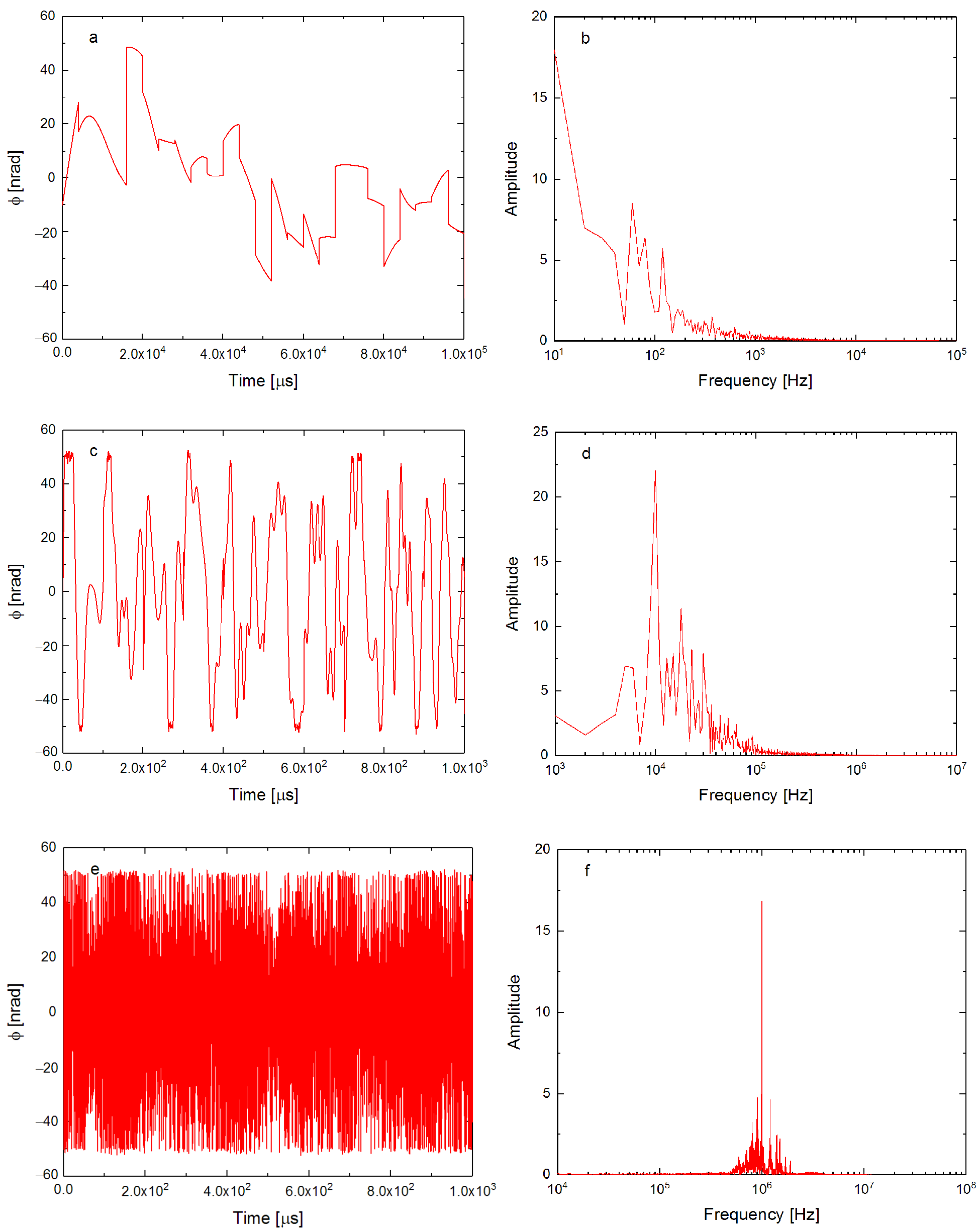
3.3. Multi-Frequency Vibrations

Due to the interference of the surrounding environment during the actual operation of the XFELO, the optical cavity is not perfectly aligned, and there is a certain amount of vibration between the various optical components. However, this vibration is a multi-frequency vibration, and the single-frequency vibration model is no longer applicable. Thus, a complex multi-frequency vibration model is needed. It is modeled by superimposing multiple sine and cosine waves and then adding random phases. This time, the multi-frequency vibration model is still built according to low frequency, medium frequency, and high frequency, where low frequency is 10 Hz as the dominant multi-frequency vibration, medium frequency is 0.01 MHz as the dominant multi-frequency vibration, and high frequency is 1 MHz as the dominant multi-frequency vibration. The simulated time and frequency domain plots of these three multi-frequency vibrations are shown in Figure 5.

The results obtained after building the model and initiating the simulation are shown in Figure 6. It can be seen from Figure 6 that the effect of multi-frequency vibrations dominated by 10 Hz and 0.01 MHz on the output laser is not significantly different compared to that of single-frequency vibrations. The energy still fluctuates around 200 μJ, the spectral bandwidths are 14.96 meV and 14.98 meV, respectively, and the beam size and beam divergence angle still fluctuate slightly around 45.35 μm and 0.34 μrad after the radiation field has saturated, similarly to the single frequency. However, for vibrations dominated by 1 MHz, the results are very different compared to single-frequency vibrations. The saturated output section has an energy maximum of 200 μJ but then undergoes a very rapid drop and does not provide a relatively constant output to the outside world. Its spectral bandwidth, beam size, and beam divergence angle are significantly changed compared to the ideal conditions. The results are very different compared to the single-frequency results at 1.1 MHz, which verifies the inference in the previous subsection. The analysis of these three multi-frequency vibrations also reveals that the saturation energy is affected more than the spectral bandwidth, beam size, and beam divergence angle as the main frequency of the vibration gradually increases. This conclusion is consistent with the analysis of the results for single-frequency vibrations in the previous section. It should be noted that the number of oscillations during the simulation was only 450. The number of oscillations is designed to be 450 because a time-dependent simulation in this condition would take approximately two days and would satisfy the needs of both medium and high frequencies. For low frequencies, 450 oscillations are not enough, as a complete cycle of mirror vibrations requires approximately 100,000 oscillations, which would take years to simulate. Therefore, we will use time-independent in subsequent simulations.

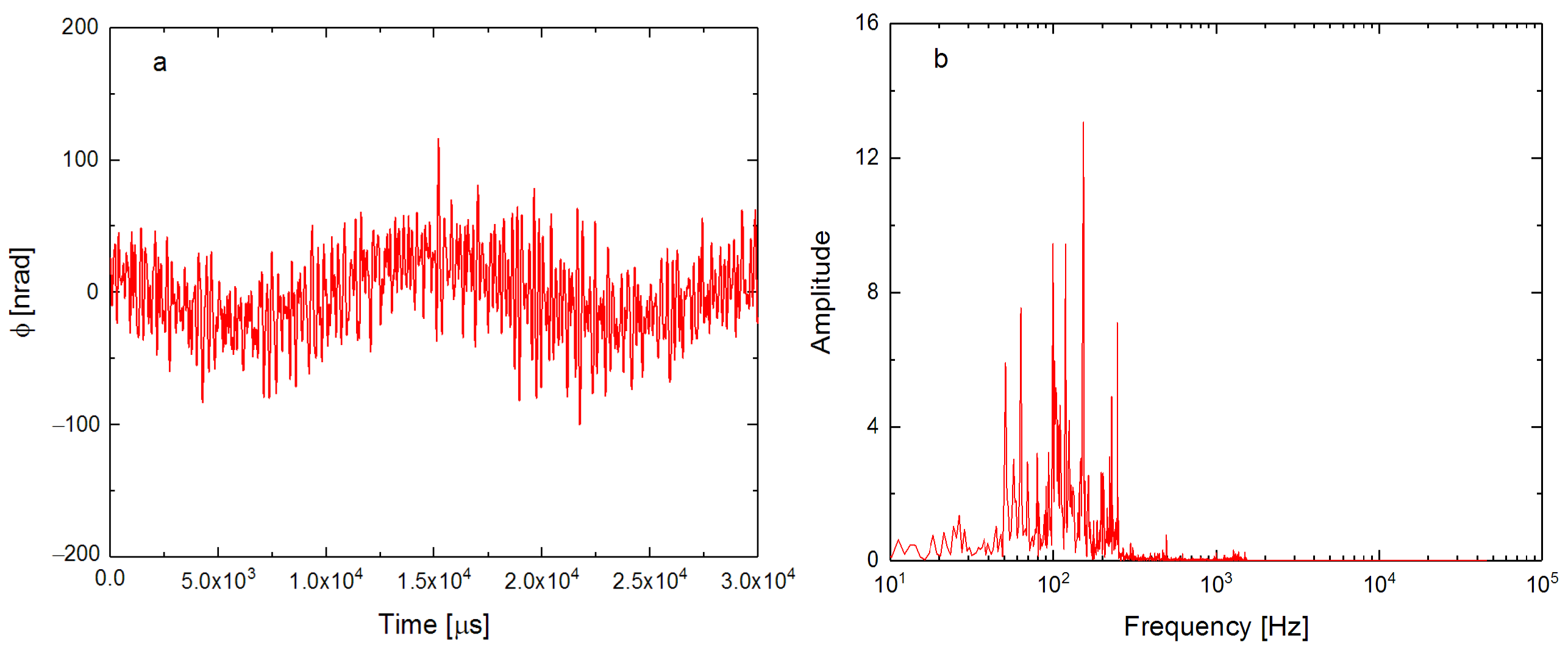
3.4. Realistic Vibration

Upon completing the multi-frequency vibration simulations, it is imperative to conduct further validation to ascertain the model’s reliability. We can do this by using measurement data from the Shanghai Synchrotron Radiation Source site. Note from Figure 3 that the measurement data are dominated by frequencies of and around 100 Hz. If the simulation is still used at 450 oscillations, these 450 oscillations will not allow the mirror to complete one cycle of vibration, and this will give an error between the results and the real results. Therefore, the number of oscillations is set here to 10,000. The time-dependent simulations in the two subsections above would take approximately two days at a time, and if this simulation still used time dependent, it would take several years. Therefore, the simulation is run using time-independent. Then, to facilitate comparison with the previous results, multi-frequency vibrations dominated by 10 Hz will be simulated. The number of vibrations is set to 100,000, and the simulation is performed using time-independent. The results of the above two simulations are shown in Figure 7.

As can be seen in Figure 7, the two simulation results reach saturation at about the same time, around oscillations of approximately 90 times. The fluctuation behavior after saturation is also quite similar. Figure 7a has a large fluctuation after the power saturation because the actual vibration main frequency is approximately 100 Hz and has a large amplitude in the initial vibration process. Similarly, Figure 7b has a small value of amplitude in the initial period, which leads to a small fluctuation of power after saturation. This conclusion can be drawn by reference to the time domain and frequency domain plots in Figure 3 and Figure 5.

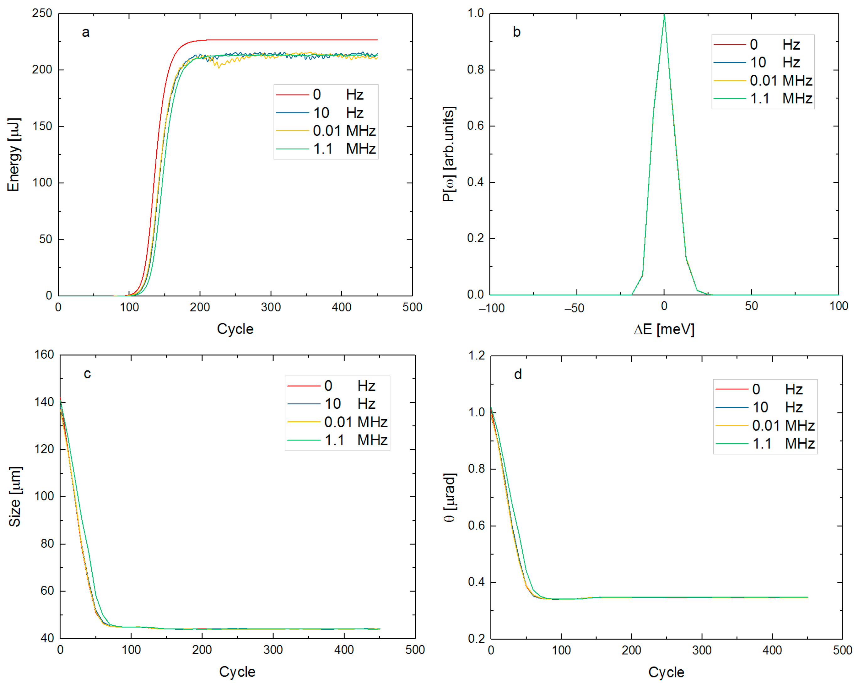
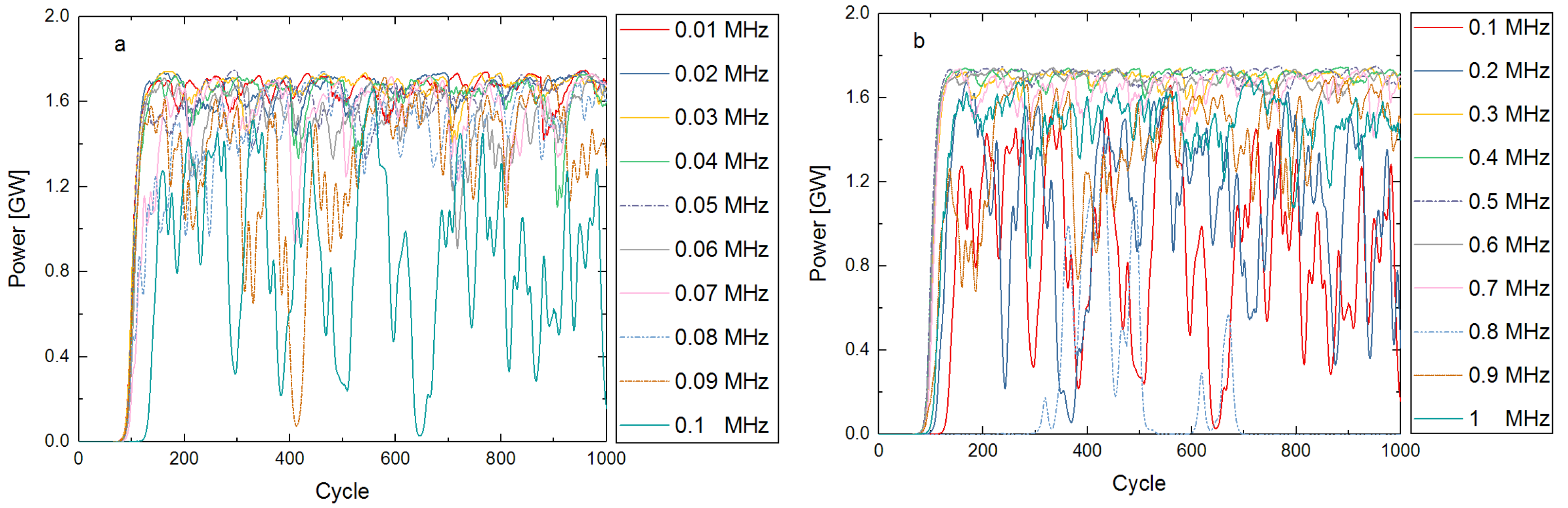
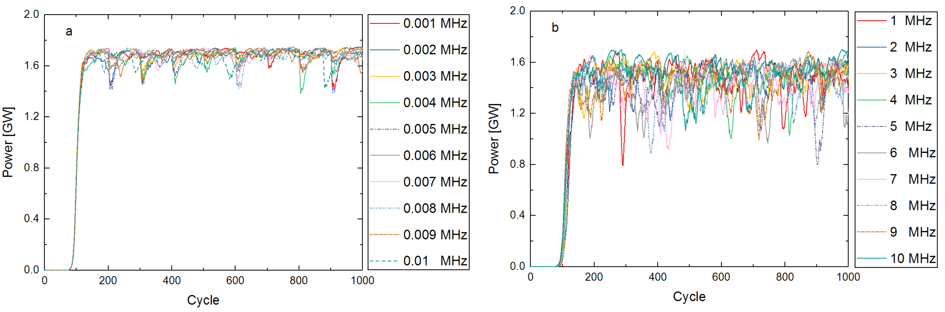
4. The Effect of Different Vibration Frequencies

As the subsequent simulations will involve low-frequency vibrations dominated by 10 Hz, all simulations are run in a time-independent manner to ensure uniformity. The number of oscillations is set to 1000 for all frequencies except for the 10–100 Hz and 100–1000 Hz multi-frequency oscillations, which are set to 100,000 and 10,000. Despite the use of time-independent simulation, the 100,000 calculation is too large, and it is expected to take two weeks to complete the oscillations. This is a choice that ensures that the number of oscillations is as uniform as possible and that the mirror completes at least one cycle of vibration for each frequency simulated.

4.1. Relationship between Frequency and Output Power

As can be seen from the third subsection of Section 3, the fluctuations of the laser saturation energy become larger with increasing mirror vibration frequency and show a decreasing trend, but these three simulations alone cannot support this inference. The frequency range is 0.01–1 MHz, and the frequency interval is chosen on the logarithmic axis as 0.01 MHz for 0.01–0.1 MHz and 0.1 MHz for 0.1–1 MHz, and the subsequent simulations are based on this criterion. The model used is the multi-frequency vibration model from the third subsection of Section 3. In order to meet the minimum frequency requirement, the number of oscillations was set uniformly to 1000, and the amplitude was taken as 50 nrad as before. Figure 8 shows the result of this simulation.

As can be seen in Figure 8, the fluctuation of the saturation power does not become as large as expected with increasing frequency when the amplitude is set to 50 nrad. When the frequency is between 0.01 MHz and 0.2 MHz, there is a significant increase in the fluctuation of the saturation optical power with increasing frequency. At frequencies of 0.08 MHz, 0.09 MHz, 0.1 MHz, and 0.2 MHz, there is even a rapid drop, but between 0.3 MHz and 0.7 MHz, the saturation power fluctuations stabilize and are close to the 0.01 MHz result. By 0.8 MHz and 0.9 MHz, the power shows a slower rise and greater fluctuations, and at 1 MHz it tends to moderate again.

Next, in order to establish whether the result above is an isolated case or exists in all frequency ranges, the frequency ranges 0.001–0.01 MHz and 1–10 MHz will be simulated with the same unchanged parameter settings as in the simulation above. The results of this simulation are shown in Figure 9. From Figure 9, it can be seen that the saturated optical power fluctuates less between 0.001 MHz and 0.01 MHz, stabilizing at approximately 1.6 GW and not showing a rapid decline. The saturation power fluctuates more in the frequency range 1–10 MHz than in the previous case and drops to approximately 1.4 GW, but like the previous case, there is no rapid drop.

To obtain a more intuitive understanding of the saturation power variation within the frequency range of 0.001–10 MHz, we analyze the data for numbers of oscillations between 200 and 1000 at each frequency. These data are then processed using a modified standard deviation formula, which can be expressed as follows:

$$\mathrm{S}=\sqrt{\frac{{\sum }_{i=1}^n{(x_i-1.76\times {10}^9)}^2}{n-1}}$$

(1)

where $1.76\times {10}^9$ is the average value of the saturation power under perfect alignment conditions. After replacing x with $1.76\times {10}^9$, the result reflects both the degree of fluctuation of the saturation power at each frequency and the decreasing trend of the power relative to the perfect alignment condition. Finally, we will obtain the scatter plot shown in Figure 10.

Combining Figure 8 and Figure 9 shows that there is a specificity in the vibration frequency of the mirror at approximately 1 MHz and 0.1 MHz. When the frequencies are dominated by 0.09 MHz, 0.1 MHz, 0.2 MHz, and 0.8 MHz, there is a large fluctuation in the saturated optical power or even a long time without a rise. At frequencies between 0.3 MHz and 0.7 MHz, the saturation power fluctuations suddenly become smaller and more stable than at most of the lower and medium frequencies. The reason for these anomalies may be related to the betatron frequency of the cavity. By performing a calculation, it can be established that the betatron frequency of our cavity is 0.15 MHz, which is close to 0.1 MHz. When the mirror vibrates at a complex frequency of 0.1 MHz, it will overlap with the betatron frequency, resulting in resonance enhancement and an excessively high red dot. An excessively low red dot is due to the frequency being aliased. As for the left side of 0.1 MHz, the effect is less because the amplitude is uniformly 50 nrad at this point, which is a relatively small amplitude. Analysis of all plots from 0.001–1 MHz shows that although special cases exist, the overall fluctuation in saturation optical power is progressively greater, and its upper limit decreases significantly.

4.2. Tolerance of Vibration Amplitude

In the previous section, the amplitude was kept constant at 50 nrad during the simulation so that the variation between the different vibration frequencies was not significant. Although Figure 10 shows the effect of different vibration frequencies on power, it is not a comprehensive summary. Therefore, the maximum amplitude tolerated for each output optical power at different vibration frequencies will be investigated. The results will be plotted to illustrate the relationship between the maximum amplitude and vibration frequency. The frequency range used in this simulation is 10 Hz–10 MHz. The number of oscillations is set to 1000 oscillations, except for 10–100 Hz and 100–1000 Hz, which are set to 100,000 and 10,000 oscillations. The tolerance limit of amplitude is determined by the ratio of the maximum power at a specific amplitude to the saturation power under ideal alignment conditions, which is less than 23%. In other words, when the maximum power is below 0.4 GW, it can be considered as reaching the amplitude tolerance limit.

An exploratory simulation of the amplitude limit is shown in Figure 11 for a multi-frequency vibration dominated by 10 Hz. Initially, simulations were conducted with amplitudes of 60 nrad and 100 nrad, revealing that the saturation power exhibited gradual fluctuations while consistently hovering around 1.6 GW. Subsequently, the ratio of the maximum power at 300 nrad to the ideal situation was found to fall below the established criterion. Moreover, the maximum power rapidly decreased after reaching its peak. Consequently, the amplitude limit for the multi-frequency vibration at 10 Hz was determined to be approximately 300 nrad. Subsequent simulations were performed with amplitudes of 250 nrad, 260 nrad, 270 nrad, 280 nrad, and 290 nrad, progressively narrowing the range of investigation to between 290 nrad and 300 nrad. Ultimately, the amplitude range of 290–300 nrad was further simulated at 1 nrad intervals, leading to the determination of the optimal amplitude at this frequency, identified as 298 nrad.

The remaining frequencies are also simulated using the method in the previous subsection to find their respective limiting amplitudes, which will eventually give the results in Figure 12. It is a scatter plot with the red dots being the frequency anomalies and the red lines being fitted after removing the anomalies. As a whole, it can be seen that as the frequency increases, there is a large drop in the power of the optical pulse for amplitude tolerance; this changes more slowly at low frequencies from 10–1000 Hz, then there is a large drop, and finally, after 1 MHz, it stabilizes again. The slow change at low frequencies is due to the fact that the amplitude of the mirror is mostly at a very low value at low frequencies, even though the amplitude is set very high. Consequently, the optical pulses are very little affected by the vibration, which ultimately leads to a slow decrease. The stabilization after 1 MHz is due to the main vibration frequency of the mirror being an integer multiple of the resonant frequency. When the laser interacts with the mirror, the amplitude of the mirror will have values that are not very different from each other. This is the reason why the tolerance change stabilizes after 1 MHz.

The same can be seen for the very low amplitude tolerance limits at 0.9 MHz, 0.8 MHz, 0.2 MHz, 0.1 MHz, 0.09 MHz, and 0.08 MHz and the anomalous high tolerance between 0.3 MHz and 0.7 MHz, which corresponds to the simulation results in the previous subsection. It is worth noting that there are also anomalies in the frequency range 0.01–0.07 MHz. This corresponds to the explanation in the previous subsection. Overall, it can be concluded that the sensitivity of the optical pulse to amplitude gradually increases when the mirror vibrates at multiple frequencies within the 10 Hz–10 MHz range. However, anomalies arise in the frequency range of 0.01–0.9 MHz, wherein the sensitivity exhibits both unusually high and low values.

5. Discussion

In summary, this paper first simulates a perfectly aligned cavity for the XFELO, then builds a simple model of a mirror vibrating at a single frequency and runs simulations to compare the results with a perfectly aligned cavity. A multi-frequency vibration model is then built based on the simple single-frequency vibration model to simulate the realistic vibration of the mirror and to investigate the variation in output optical pulse energy, spectral bandwidth, beam size, and beam divergence angle for different vibration frequencies. This is followed by simulations using a set of realistic measurements from SSRF to verify the feasibility of the multi-frequency vibration model. After verifying the feasibility of the model, we simulate the multi-frequency vibration of the mirror in the range of 10 Hz–10 MHz to find the maximum amplitude tolerated for the optical pulse at different vibration frequencies and analyzed the relationship between the maximum amplitude and frequency. The results show that a gradual increase in the sensitivity of optical pulses to amplitude with increasing frequency. In fact, the frequencies during vibration primarily revolve around the low and medium ranges. Vibrations of approximately 10 Hz can be offset by increasing feedback. Although there is no way to offset the vibration of 100–1000 Hz effectively, Figure 12 shows that the output power at this frequency has a high tolerance for the amplitude, which is approximately 250 nrad or more. Therefore, the vibration of this frequency has little effect on the output laser in the actual operation. Notably, abnormal frequencies within the range of 0.01–1 MHz exhibit exceptional sensitivity, either excessively high or low. There is great instability in this part of the vibration, and small perturbations can have a huge impact on the output laser. It is also worth noting that the slow change in sensitivity of the optical pulse to amplitude after 1 MHz is due to the design of the optical cavity structure. The structure is based on the design of a superconducting linear accelerator at SHINE, and the change in sensitivity of this part will not be the same when the accelerator is different.

References

1. Bostedt, C.; Boutet, S.; Fritz, D.M.; Huang, Z.; Lee, H.J.; Lemke, H.T.; Robert, A.; Schlotter, W.F.; Turner, J.J.; Williams, G.J. Linac coherent light source: The first five years. Rev. Mod. Phys. 2016, 88, 015007. [Google Scholar] [CrossRef]
2. Huang, N.; Deng, H.; Liu, B.; Wang, D.; Zhao, Z. Features and futures of X-ray free-electron lasers. Innovation 2021, 2, 1–19. [Google Scholar] [CrossRef] [PubMed]
3. Feng, C.; Deng, H.-X. Review of fully coherent free-electron lasers. Nucl. Sci. Tech. 2018, 29, 160. [Google Scholar] [CrossRef]
4. Huang, Z.; Kim, K.-J. Review of X-ray free-electron laser theory. Phys. Rev. Spec. Top.-Accel. Beams 2007, 10, 034801. [Google Scholar] [CrossRef]
5. Kondratenko, A.; Saldin, E. Generating of coherent radiation by a relativistic electron beam in an ondulator. Part. Accel. 1980, 10, 207–216. [Google Scholar]
6. Derbenev, Y.S.; Kondratenko, A.; Saldin, E. On the possibility of using a free electron laser for polarization of electrons in storage rings. Nucl. Instrum. Methods Phys. Res. 1982, 193, 415–421. [Google Scholar] [CrossRef]
7. Bonifacio, R.; Pellegrini, C.; Narducci, L. Collective instabilities and high-gain regime in a free electron laser. Opt. Commun. 1984, 50, 373–378. [Google Scholar] [CrossRef]
8. Kim, K.-J.; Shvyd’ko, Y.; Reiche, S. A proposal for an X-ray free-electron laser oscillator with an energy-recovery linac. Phys. Rev. Lett. 2008, 100, 244802. [Google Scholar] [CrossRef]
9. Huang, Z.; Ruth, R.D. Fully coherent X-ray pulses from a regenerative-amplifier free-electron laser. Phys. Rev. Lett. 2006, 96, 144801. [Google Scholar] [CrossRef]
10. Dai, J.; Deng, H.; Dai, Z. Proposal for an X-ray free electron laser oscillator with intermediate energy electron beam. Phys. Rev. Lett. 2012, 108, 034802. [Google Scholar] [CrossRef]
11. Rauer, P.; Decking, W.; Lipka, D.; Thoden, D.; Wohlenberg, T.; Bahns, I.; Brueggmann, U.; Casalbuoni, S.; Di Felice, M.; Dommach, M. Cavity based X-ray free electron laser demonstrator at the European X-ray Free Electron Laser facility. Phys. Rev. Accel. Beams 2023, 26, 020701. [Google Scholar] [CrossRef]
12. Lindberg, R.; Kim, K.-J.; Shvyd’ko, Y.; Fawley, W. Performance of the X-ray free-electron laser oscillator with crystal cavity. Phys. Rev. Spec. Top.-Accel. Beams 2011, 14, 010701. [Google Scholar] [CrossRef]
13. Li, K.; Deng, H. Gain-guided X-ray free-electron laser oscillator. Appl. Phys. Lett. 2018, 113, 061106. [Google Scholar] [CrossRef]
14. Huang, N.; Deng, H. Generating X-rays with orbital angular momentum in a free-electron laser oscillator. Optica 2021, 8, 1020–1023. [Google Scholar] [CrossRef]
15. Shvyd’ko, Y.V.; Stoupin, S.; Cunsolo, A.; Said, A.H.; Huang, X. High-reflectivity high-resolution X-ray crystal optics with diamonds. Nat. Phys. 2010, 6, 196–199. [Google Scholar] [CrossRef]
16. Shvyd’Ko, Y.; Lindberg, R. Spatiotemporal response of crystals in X-ray Bragg diffraction. Phys. Rev. Spec. Top.-Accel. Beams 2012, 15, 100702. [Google Scholar] [CrossRef]
17. Snigirev, A.; Kohn, V.; Snigireva, I.; Lengeler, B. A compound refractive lens for focusing high-energy X-rays. Nature 1996, 384, 49–51. [Google Scholar] [CrossRef]
18. Kolodziej, T.; Stoupin, S.; Grizolli, W.; Krzywinski, J.; Shi, X.; Kim, K.-J.; Qian, J.; Assoufid, L.; Shvyd’ko, Y. Efficiency and coherence preservation studies of Be refractive lenses for XFELO application. J. Synchrotron Radiat. 2018, 25, 354–360. [Google Scholar] [CrossRef]
19. Batterman, B.W.; Cole, H. Dynamical diffraction of X-rays by perfect crystals. Rev. Mod. Phys. 1964, 36, 681. [Google Scholar] [CrossRef]
20. Huang, N.; Deng, H. Thermal loading on crystals in an X-ray free-electron laser oscillator. Phys. Rev. Accel. Beams 2020, 23, 090704. [Google Scholar] [CrossRef]
21. Tiwari, G.; Lindberg, R.R. Misalignment effects on the performance and stability of X-ray free electron laser oscillator. Phys. Rev. Accel. Beams 2022, 25, 090702. [Google Scholar] [CrossRef]
22. Qi, P.; Shvyd’ko, Y. Signatures of misalignment in X-ray cavities of cavity-based X-ray free-electron lasers. Phys. Rev. Accel. Beams 2022, 25, 050701. [Google Scholar] [CrossRef]
23. Kim, K.-J.; Huang, Z.; Lindberg, R. Synchrotron Radiation and Free-Electron Lasers; Cambridge University Press: Cambridge, UK, 2017. [Google Scholar]
24. Huang, N.-S.; Liu, Z.-P.; Deng, B.-J.; Zhu, Z.-H.; Li, S.-H.; Liu, T.; Qi, Z.; Yan, J.-W.; Zhang, W.; Xiang, S.-W. The MING proposal at shine: Megahertz cavity enhanced X-ray generation. Nucl. Sci. Tech. 2023, 34, 6. [Google Scholar] [CrossRef]
25. Yang, H.; Yan, J.; Deng, H. High-repetition-rate seeded free-electron laser enhanced by self-modulation. Adv. Photonics Nexus 2023, 2, 036004. [Google Scholar] [CrossRef]
26. Reiche, S. GENESIS 1.3: A fully 3D time-dependent FEL simulation code. Nucl. Instrum. Methods Phys. Res. Sect. A Accel. Spectrometers Detect. Assoc. Equip. 1999, 429, 243–248. [Google Scholar] [CrossRef]
27. van der Slot, P.J.; Freund, H.; Miner, W., Jr.; Benson, S.; Shinn, M.; Boller, K.-J. Time-dependent, three-dimensional simulation of free-electron-laser oscillators. Phys. Rev. Lett. 2009, 102, 244802. [Google Scholar] [CrossRef]
28. Huang, N.-S.; Li, K.; Deng, H.-X. BRIGHT: The three-dimensional X-ray crystal Bragg diffraction code. Nucl. Sci. Tech. 2019, 30, 39. [Google Scholar] [CrossRef]
Figure 1. The cavity structure of the XFELO, where M 1 , M 2 , M 3 , a n d   M 4 are the four diamond crystal mirrors and the CRL is the focusing element.
Photonics 10 01058 g001
Figure 2. Numerical simulation results for perfect alignment conditions, where (a) is a plot of output energy that varies with the number of oscillations, (b) is a plot of the output laser spectrum, and (c) and (d) are plots of beam size and divergence angle, which vary with the number of oscillations.
Photonics 10 01058 g002
Figure 3. Time and frequency domain plots of the vibration of SHINE. (a) is the time domain plot, where the vertical axis ϕ indicates the radian of the mirror vibration, and (b) is the frequency domain plot.
Photonics 10 01058 g003
Figure 4. Effect of three single-frequency oscillations at 1.1 MHz, 0.01 MHz, and 10 Hz on laser output energy, spectral bandwidth, beam size, and beam divergence angle at an amplitude of 50 nrad, where (a) is a plot of the energy that varies with the number of oscillations, (b) is a plot of the output laser spectrum, and (c,d) are plots of the beam size and beam divergence angle, which vary with the number of oscillations. The vertical axis θ of (d) indicates the laser divergence angle at the oscillator’s exit.
Photonics 10 01058 g004
Figure 5. (a,b) are time and frequency domain plots of the mirror when vibrating at 10 Hz as the dominant multi-frequency, (c,d) are time and frequency domain plots of the mirror when vibrating at 0.01 MHz as the dominant multi-frequency, and (e,f) are time and frequency domain plots of the mirror when vibrating at 1 MHz as the dominant multi-frequency. The amplitudes of these three multi-frequency vibrations are set at approximately 50 nrad.
Photonics 10 01058 g005
Figure 6. Plots of simulation results when the mirror vibrates at low (dominated by 10 Hz), medium (dominated by 0.01 MHz), and high (dominated by 1 MHz) frequencies, where (ad) are plots of output energy that varies with the number of oscillations, plots of output laser spectrum, plots of beam size, and beam divergence angle that varies with the number of oscillations, respectively.
Photonics 10 01058 g006
Figure 7. The plots of power variation with the number of oscillations, where (a) is the result of a simulation using actual measurement data and (b) is the result of a simulation using a multi-frequency vibration model dominated by 10 Hz. The subplots of (a,b) represent the results for the first 500 oscillations.
Photonics 10 01058 g007
Figure 8. Plot of the variation of optical power with the number of oscillations at different vibration frequencies. The frequency range represented by (a) is 0.01–0.1 MHz and by (b) is 0.1–1 MHz.
Photonics 10 01058 g008
Figure 9. Plot of the variation of optical power with the number of oscillations at different vibration frequencies. The frequency range represented by (a) is 0.001–0.01 MHz and by (b) is 1–10 MHz.
Photonics 10 01058 g009
Figure 10. Scatter plot indicating the degree of saturation power fluctuation, where the red points are anomalies and the red line is the fitted line after removing these anomalies.
Photonics 10 01058 g010
Figure 11. Plot of the variation of power with the number of oscillations for different amplitudes when the vibration frequency is a multi-frequency vibration dominated by 10 Hz. Where (a) the amplitudes are 50 nard, 60 nrad, 100 nrad, 200 nrad, 250 nrad, 260 nrad, 270 nrad, 280 nrad, 290 nrad, 300 nrad, and (b) the amplitudes are 291–299 nrad.
Photonics 10 01058 g011
Figure 12. Scatter plot of the one-to-one correspondence between the maximum vibration amplitude tolerated by the laser power and the frequency.
Photonics 10 01058 g012