Automated Segmentation and Morphometry of Zebrafish Anterior Chamber OCT Scans

Abstract

Zebrafish (Danio rerio) eyes are widely used in modeling studies of human ophthalmic diseases, including glaucoma and myopia. These pathologies cause morphological variations in the anterior chamber elements, which can be quantitatively measured using morphometric parameters, such as the corneal curvature, central corneal thickness, and anterior chamber angle. In the present work, an automated method is presented for iris and corneal segmentation, as well as the determination of the above-mentioned morphometry from optical coherence tomography (OCT) scans of zebrafish. The proposed method consists of four stages; namely, preprocessing, segmentation, postprocessing, and extraction of morphometric parameters. The first stage is composed of a combination of wavelet and Fourier transforms as well as gamma correction for artifact removal/reduction. The segmentation step is achieved using the U-net convolutional neural network. The postprocessing stage is composed of multilevel thresholding and morphological operations. Finally, three algorithms are proposed for automated morphological extraction in the last step. The morphology obtained using our automated framework is compared against manual measurements to assess the effectiveness of the method. The obtained results show that our scheme allows reliable determination of the morphometric parameters, thereby allowing efficient assessment for massive studies on zebrafish anterior chamber morphology using OCT scans.

1. Introduction

The anterior chamber refers to the front part of the eye between the cornea and iris that contains the aqueous humor. The aqueous humor flows from the ciliary body into the anterior chamber and is drained out through spongy tissue called the trabecular meshwork into the Schlemm’s canal [1]. The aqueous humor provides nutrition to the eye and retains the intraocular pressure (IOP). When drainage problems occur by a narrowed fluid exit, fluid flow is disturbed as well as causing the IOP to be increased [1,2]. Increased IOP by a narrowed Schlemm’s canal can also lead to pathogenesis of angle-closure glaucoma and morphological changes in the tissues of the anterior chamber [3,4,5]. Hence, observation of the anterior chamber morphology is one of the methods for diagnosing ophthalmic diseases, including glaucoma [5,6,7,8].

The zebrafish is chosen as an animal model to observe the morphological changes in the anterior chamber segment. Zebrafish (Danio rerio) has been used as a useful model organism in medical and pharmaceutical research owing to its genetic similarity to humans, as well as relatively easier breeding and maintenance than other animal models [9,10]. Despite the advantages gained from the use of zebrafish, there are problems with extracting reliable data from their eye morphology in large populations, owing to limitations with reliable and fast image-analysis tools. For example, the corneal thickness of the zebrafish reported by Zhao et al. was approximately 20 $\mathsf{\mu }$m by the analysis of histologic sections using light microscopy, whereas the results obtained by Heur et al. showed an approximate thickness of 46.5 $\mathsf{\mu }$m using spectral-domain OCT (SD-OCT) techniques [11,12]. These suggest that the baseline research on the dimensions of ocular structures in the zebrafish eye have to be repeated to validate existing results and produce normative datasets that would allow reliable studies of eye diseases in the future. Such a study is also expected to provide the criteria and references to identify zebrafish with abnormal eye growths and assess the health statuses of zebrafish eyes. In comparisons between disease models and improved age-matched controls, wild-type zebrafish enable enhanced reliability of experiments in the disease models. Therefore, automatic image processing and morphometry extraction are required to achieve reliable measurements and to create a database of the anterior chamber morphologies of age-matched controls using massive populations of zebrafish.

For human eye scans analysis, different proposals for the automated anterior chamber elements segmentation using deep learning algorithms have been previously published. Measurements such as angle closure and scleral spur locations have been proposed by Xu et al. [13]. Also, a more complete quantification of several elements was published by Pham et al. [14]: a proposal whose main algorithm relies on the use of a hybrid proposal between three different neural networks, providing accurate segmentation of elements such as lens vault (LV), iris thickness (IT), trabecular iris space area, among many others. However, regarding zebrafish scans, an automated segmentation or measurement method of anterior chamber elements has not been reported. Taking into account the few morphological differences between the human and zebrafish eye [15,16], a new method for this proposal has to be developed. Many anterior chamber parameters can be acquired in human eyes, for example, anterior chamber angle (ACA), anterior chamber depth (ACD), anterior chamber width (ACW), angle opening distance (AOD), iris-ciliary process distance (ICPD), iris–lens contact distance (ILCD), trabecular-iris angle (TIA), and trabecular-iris space area (TISA). However, zebrafish eyes have some limitations in measuring all parameters. First, zebrafish have a strongly reflective iris, which disturbs the measurements of the trabecular-iris space area/angle recess area and angle opening distance. Second, unlike in human eyes, the zebrafish lens is located very close to the cornea, so that measuring the central anterior chamber area or depth is impossible.

In the present work, an automated method is presented for corneal and iris segmentation and extraction of the anterior chamber morphometry from zebrafish images. The anterior chamber images of zebrafish were obtained using a custom-built optical coherence tomography (OCT) system for automated extraction of three morphometric parameters; namely, corneal curvature (CC), central corneal thickness (CCT), and anterior chamber angle (ACA): ocular parameters where anterior chamber elements are involved and modified regarding the morphological changes described above. The CCT is an essential parameter in assessing any potential glaucoma and eye diseases, since it plays an important role in the IOP variations [4,17], where thinner CCT is related to several factors, which are indicators of glaucoma progression and adjacent damage [18]. On the other hand, the ACA is a closely related parameter identified as causative for human primary open glaucoma [19], where the zebrafish has been employed as a model [20]. Last but not least, the CC is one of the essential parameters when calculating the refractive power of the eye. Also, it has a strong and inverse correlation when measuring the CCT [21].

2. Methods

In this section, the optical system configuration, image acquisition protocols, and image processing steps are described in detail. To obtain measurements of the morphometric parameters noted previously, it is necessary to first segment the cornea and iris. The processing of OCT scans can be divided into three stages; namely, preprocessing, segmentation, and postprocessing. Once the key structures are segmented, the ocular morphology is extracted using the distances between the ocular structures, as summarized in Figure 1.

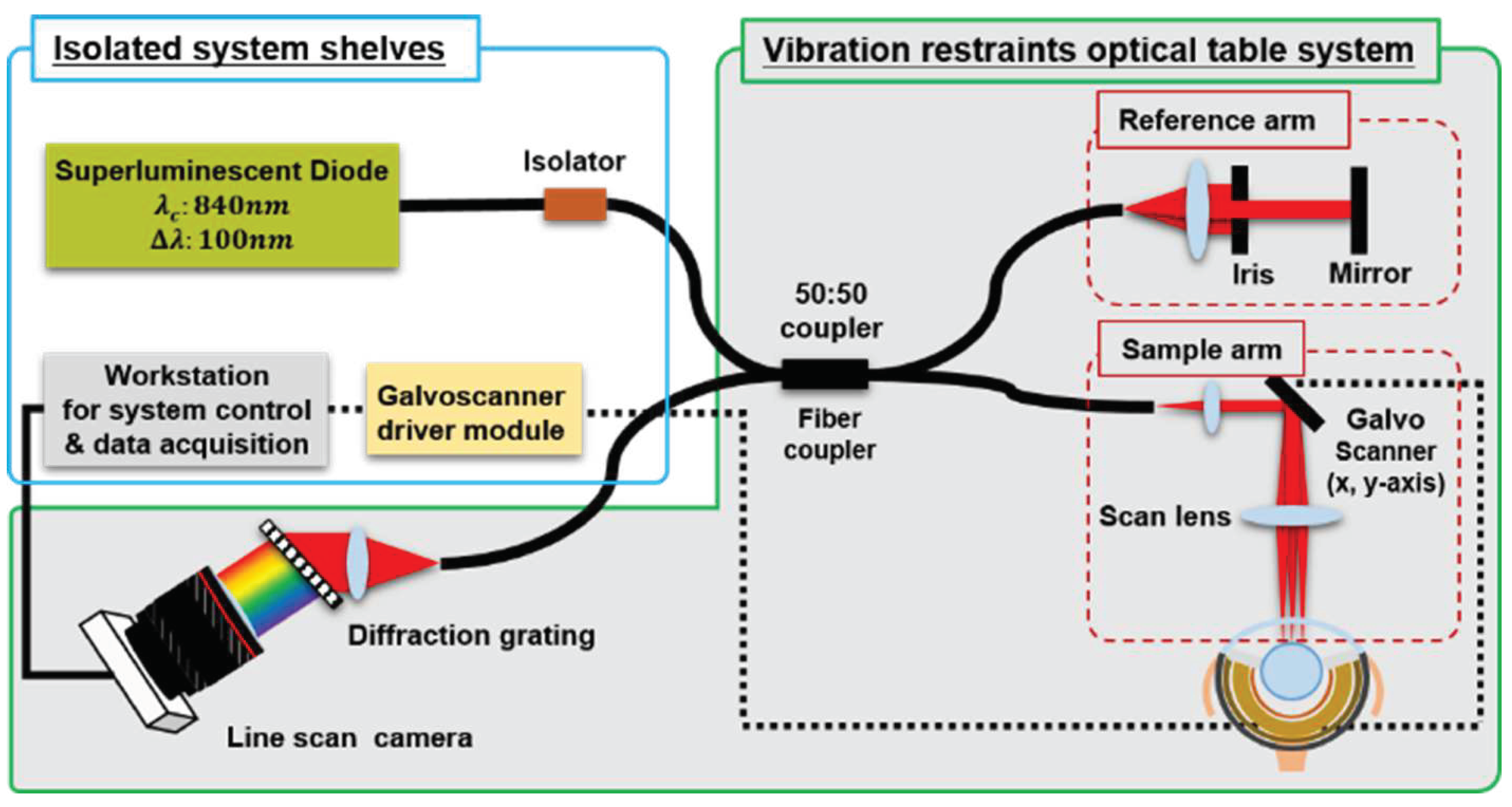
2.1. Imaging System Setup

Anterior chamber images of zebrafish eyes were acquired using a custom-built OCT system with a fiber-coupled light source and 50:50 directional fiber coupler that splits the light between the reference and sample arms. The reference arm constitutes a high-reflectance mirror and iris (diaphragm) to control the power. The light source (bandwidth $\Delta \lambda$: 100 nm, central wavelength ${\lambda }_c$: 840 nm) provides a theoretical axial resolution of approximately 3 $\mathsf{\mu }$m in air (M-D-840HP SUPERLUM, Carrigtwohill, Ireland). A two-axis galvo-scanner set (8315K custom scanner set, Cambridge Technology, Bedford, MA, USA) is used in the sample arm for raster scanning of the sample to generate volume images. This OCT-detection system was calibrated using a spectroscopic fitting method based on the absolute wavenumber calibration at a set of discrete pixel locations and additional numerical dispersion compensation [22]. A vibration restraints optical table system prevented the vibration of the control system and the affections by unspecific forces. The illustration of this OCT system is shown in Figure 2.

2.2. Zebrafish Image Acquisition Protocol

Ten in-water anesthetized wild-type zebrafish were used to obtain the volumetric images of the anterior chamber. The zebrafish’s age was eight months, corresponding to adults in the life cycle of the zebrafish. The anesthesia procedures are described in previous research, as well as the zebrafish information network (ZFIN, an online biological database of information about zebrafish) [23]. All imaging procedures were in compliance with the experimental protocols approved by the Institutional Animal Care and Use Committee of Inha University (approval number: 200901-717). After acquiring the volumetric data, standard OCT processing was applied to create serial images and the axial pixel spacing was calibrated by considering a refractive index of 1.34 for the zebrafish cornea [24]. The theoretical axial pixel size of the OCT system is 1.551 $\mathsf{\mu }$m in the air (refractive index: 1). The algorithm used for the axial pixel calibration is from the previous research reported by Z. Turani et al. in 2018 [25]. In addition, the axially calibrated images were resized to match a geometrical aspect ratio of 1:1 (457 × 1754 pixels corresponding to an area of 0.88 × 3.375 mm).

2.3. Image Preprocessing

Before applying segmentation, it is important to enhance the contrast of the OCT images to avoid segmentation errors. Different preprocessing techniques have already been used and reported for human and animal OCT scans depending on the artifact types present in the images, such as A-line and saturation removal [26], wavelet-based speckle denoising [27], and motion artifact reduction [28]. In the present study, two steps were applied during preprocessing; the vertical and horizontal stripes in the images were removed first, and the brightness of the composite elements were then adjusted by gamma correction. A summary of the above-mentioned steps is shown in Figure 3.

2.3.1. Wavelet + Fourier Transforms for Stripe Removal

The zebrafish anterior chamber OCT scans often have vertical and horizontal stripe artifacts owing to high tissue reflectivity; it is, therefore, important to preprocess the images before segmentation to improve image quality.

As can be seen in Figure 3a, the zebrafish anterior chamber OCT B-scan shows vertical and horizontal stripes; these artifacts are attributed to the local saturation of the OCT detector. To reduce the artifacts caused by such saturation, stripe removal using a combined wavelet and Fourier transform approach proposed by Münch et al. [29] is applied, which results in improved images compared to the purely fast Fourier transform (FFT)-based stripe removal. In Figure 3b, the horizontal and vertical stripes removed from the original OCT B-scan are shown. The usefulness of this method lies in the preservation of the structural features by using the FFT on the Wavelet domain, providing a stricter separation between original structures and artifacts.

In general, this algorithm works as follows: by applying a wavelet transform to the image, a decomposition of three different wavelets is obtained, where each component stores structural information about the horizontal, vertical, and diagonal details. Let us consider the input image as a two-dimensional function I(x,y) of size M × N, and the discrete wavelet transform (DWT) is defined in (1) and (2):

$$W_{\phi }(j_0,m,n)=\frac{1}{\sqrt{MN}}\sum _{x=0}^{M-1}\sum _{y=0}^{N-1}I(x,y){\phi }_{j_0,m,n}(x,y)$$

(1)

$$W_{\psi }^i(j,m,n)=\frac{1}{\sqrt{MN}}\sum _{x=0}^{M-1}\sum _{y=0}^{N-1}I(x,y){\psi }_{j,m,n}^i(x,y)i=\{H,V,D\}$$

(2)

where the separable wavelets with directional sensitivity for the horizontal (H), vertical (V), and diagonal (D) components are defined in (3), (4), and (5), respectively:

$${\psi }^H(x,y)=\psi \left(x\right)\phi \left(y\right)$$

(3)

$${\psi }^V(x,y)=\phi \left(x\right)\psi \left(y\right)$$

(4)

$${\psi }^D(x,y)=\psi \left(x\right)\psi \left(y\right)$$

(5)

The scaled and translated basis functions for the DWT are expressed as in (6) and (7):

$${\phi }_{j,m,n}(x,y)=2^{j/2}\phi (2^{j}x-m,2^{j}y-n)$$

(6)

$${\psi }_{j,m,n}^i(x,y)=2^{j/2}{\psi }^i(2^{j}x-m,2^{j}y-n),i=\{H,V,D\}$$

(7)

For more detailed mathematical analyses, please refer to [30]. Once the wavelet components ${\psi }^H(x,y)$ and ${\psi }^V(x,y)$ are obtained, the DFT is applied to transform the image to the frequency domain, where the stripe artifacts are contained in the high-frequency components. This process is applied eight times, i.e., up to decomposition level L = 8, to ensure the removal of the stripe residuals. The DWT is performed using the Daubechies 22 wavelet set. Considering the horizontal and vertical wavelet components ${\psi }^H(x,y)$ and ${\psi }^V(x,y)$, respectively, which are composed of eight different decompositions of different $A\times B$ sizes, the DFT is defined in (8):

$$F_{\psi }^i(u,v)=\frac{1}{AB}\sum _{x=0}^{A-1}\sum _{y=0}^{B-1}{\psi }^i(x,y)exp\left[-j2\pi \left(\frac{ux}{A}+\frac{vy}{B}\right)\right],i=\{H,V\}$$

(8)

Here, a bandpass filter is applied to the Fourier coefficients using a Gaussian filter for both the vertical and horizontal coefficients, as defined in (9):

$$H(u,v)=F_{\psi }^i(u,v)\left(1-exp\left(\frac{-D^2(u,v)}{2{\sigma }^2}\right)\right)$$

(9)

where $\sigma$ represents the standard deviation of the Gaussian function, which is set as 1.

Once the stripes are removed, it is necessary to transform the image back to the spatial domain to produce the image $I^{\prime }(x,y)$. This is achieved with the inverse discrete Fourier transform (IDFT) as well as the inverse DWT (IDWT), which are mathematically expressed by (10) and (11), respectively:

$$f_{\psi }^i(x,y)=\sum _{u=0}^{A-1}\sum _{v=0}^{B-1}H(u,v)exp\left[j2\pi \left(\frac{ux}{A}+\frac{vy}{B}\right)\right],i=\{H,V\}$$

(10)

$$\begin{array}{cc}\hfill I^{\prime }(x,y)& =\frac{1}{\sqrt{MN}}\sum _m\sum _n{W}_{\phi }(j_0,m,n){\phi }_{j_0,m,n}(x,y)\hfill \\ \hfill & +\frac{1}{\sqrt{MN}}\sum _{i=H,V,D}\sum _{j=j_0}^{\infty }\sum _m\sum _n{W}_{\psi }^i(j,m,n)f_{\psi j,m,n}^i(x,y),i=\{H,V,D\}\hfill \end{array}$$

(11)

Since the DFT uses a frequency-domain-filtering process, the scan loses luminance and shows grayish regions. To homogenize and recover the contrast of the image elements, gamma correction is applied, as detailed below.

2.3.2. Gamma Correction

The fundamental principle of gamma correction is in the well-known power-law transformation [30] expressed in (12):

$$G=a{P}^{\gamma }$$

(12)

where a and $\gamma$ are positive real-valued constants, P is the pixel value ($P\in [0,255]$ for an 8-bit grayscale image), and G is the corrected pixel value. Conventionally, the exponent of this transformation is usually the letter gamma, which represents the algorithm name. When calculating the pixel intensity compensation, the input pixel value is raised to the power of the inverse of gamma ($\gamma$), whose value is known [31]. Considering this, (12) is applied to the grayscale values, and by considering $a=1$, the inverted gamma correction is mathematically expressed as in (13):

$$G=255{\left(\frac{P}{255}\right)}^{\frac{1}{\gamma }}$$

(13)

Figure 4 shows a plot of G versus P for different $\gamma$ values. The variable L represents the maximum input pixel value. It is observed that opposite responses are obtained for $\gamma >1$ and $\gamma <1$. As the $\gamma$ values move farther away from 1, more drastic responses are observed. As the $\gamma$ value approaches zero (known as encoding gamma), the pixel values are brighter; otherwise, as the $\gamma$ value passes unity (known as decoding gamma), the pixels become less bright. In this work, $\gamma =1.1$ is used to recover the contrast of the B-scan images. As shown above, in Figure 3c, the stripes are removed, and the contrast is recovered. Once the preprocessing is completed, segmentation is applied as detailed next.

2.4. Segmentation Process

Before performing segmentation and due to the fact that a training dataset is required for convolutional neural network (CNN)-based segmentation, manual segmentation was conducted. Both the manual and CNN-based segmentation steps are detailed below.

2.4.1. Manual Multilabel Segmentation and Data Labeling

To train the network, ground truth images (training dataset) are necessary. Manually segmented images were obtained using the ImageJ software developed by the National Institutes of Health (NIH). From the preprocessed scans obtained from the ten different zebrafish, 65 central scans were randomly selected. In each scan, both the iris and cornea were manually segmented, as shown in Figure 5. The segmentation of the cornea is limited to its junction with the iris, as further consideration is unnecessary for the purposes of this method. The delineation of central corneal thickness followed the criteria proposed by Heur et al. [12]. Corneal-edge pixels are quite defined in pre-processed scans. On the other hand, even having the presence of glare pixels around the iris, manual segmentation is straightforward since pixels corresponding to the iris are well-saturated.

2.4.2. CNN-Based Cornea and Iris Segmentation

CNNs have been widely used for medical image segmentation, given their success and efficiency, including proposals for ophthalmic scans, such as retinal vessel segmentation and retinal layer segmentations [32,33]. For the segmentation of images of the anterior eye structures, several architectures have been used, such as faster region-based CNN (FR-CNN) [34], PIPE-Net [35], and Lenet-5 [36]. Different networks have been developed for training using smaller numbers of images with improved levels of success. One of the most used architectures, because of its efficiency with a fewer number of training images, is the so-called U-net, which has been widely used for the task of medical image segmentation [37]. It was introduced by Ronneberger et al. [38] and was initially designed for electron microscopy images, but has also been used on images acquired from different modalities [39,40]. The U-net has been proven to provide good results for segmenting eye-related images [41,42], and considering the low computational cost and great performance with limited training data, this architecture is selected for the segmentation stage. This architecture is composed of encoder and decoder paths. The first one captures the context and extracts high-level features from the input image by using convolutional layers with max-pooling operations. On the other hand, the second generates the segmentation mask by upsampling and combining the features from the encoder. In addition, to preserve the fine-grained details, skip connections are added to enable the flow of information from lower-resolution feature maps to higher-resolution ones, facilitating the precise localization of objects in the segmentation mask. By applying a 1 × 1 convolution followed by a softmax activation function, the final layer generates a pixel-wise probability map that represents the predicted segmentation mask.

Geometric data augmentation was performed over the 65 scans to obtain a larger training dataset, in which image inversion techniques, as well as horizontal and vertical displacements, were used. Thus, a total of 260 images were used to train the network. For the work presented herein, the scans were resized to 128 × 128 pixels resolution, since there was not any performance impact on using a higher resolution, but it kept the computational cost lower. The whole dataset was shuffled and divided into training and test sets in a ratio of 80:20 and a stratified 5-fold cross-validation technique [43] is used, considering the limited sample. This technique yielded softmax outputs using a binary cross-entropy loss function. After a fine-tuning process, the Adam optimizer [44] was implemented with a learning rate of $1\times {10}^{-4}$; the training process was completed for 20 epochs with 1000 steps per epoch.

2.5. Postprocessing

For the probability map obtained through the U-net, each pixel has a value weight depending on its degree of coincidence with the ground truth, as shown in Figure 6a. The postprocessing step is then applied to the map to obtain a final segmentation prior to the measurement of the parameters. First, thresholding is applied based on the range of values in the map. In this work, it is necessary to segment three eye structures (background, iris, and cornea) so that two normalized threshold values are proposed; namely, $t{h}_1$ and $t{h}_2$, with values of 0.25 and 0.65, respectively. Let us consider $p(x,y)$ as the probability map. The function $s(x,y)$ that assigns the probability values to allow image segmentation is defined in (14):

$$s(x,y)=\left\{\begin{array}{cc}0\hfill & \mathrm{if}p(x,y)<t{h}_1\hfill \\ 128\hfill & \mathrm{if}t{h}_1<p(x,y)<t{h}_2\hfill \\ 255\hfill & \mathrm{if}p(x,y)>t{h}_2\hfill \end{array}\right.$$

(14)

where the values for the background, iris, and cornea are 0, 128, and 255, respectively.

Once the threshold values are set, the morphological operations are performed to better profile each element: a technique that has been widely used as postprocessing in different approaches. A combination of dilation and erosion operations is applied to compensate for the pixels representing the junction between the iris and cornea, which is often misinterpreted. Derived from the thresholding process, the morphological operations can be applied to each of the segmented structures separately, since their pixel values are different. For example, as shown in Figure 6, the obtained probability map considers the outer part of the cornea as the iris. This is easily compensated by applying the dilation operation followed by the erosion operation to the pixels corresponding to the cornea, so that the pixels detected as iris are completed. The final segmentation results are shown in Figure 6b.

2.6. Automated Measurements

Once the iris and corneal zones are segmented, custom pixelwise algorithms are implemented to measure the ACA, CCT, and CC. The measurement algorithm for each parameter is described below.

2.6.1. Anterior Chamber Angle (ACA)

Considering that standardized measurement techniques of the ACA or iridocorneal angle in zebrafish scans are not well-defined [20,45], an analysis similar to that performed with images of the human eye anterior segments is proposed. In the human eyes, the angle opening distance (AOD) at 500 $\mathsf{\mu }$m (AOD500) is one of the standard extracted parameters for ACA measurement [46], since it is used as the distance where the angle must be measured. This parameter was first used on ultrasound biomicroscopic images and was proposed by Pavlin et al. [47] in 1992. To obtain the proportional distance of the AOD500 to measure the ACA in zebrafish, the anterior chamber width (ACW) [48] was considered for a scaled proportional analysis. A study presented by Goldsmith et al. [49] on 20 human patients’ scans reported an ACW average of $12.53\pm 0.47$ mm (inter eye SD). The ACW was manually measured from the selected scans, and the obtained mean value was $1.38\pm 0.10$ mm (detailed values are presented in Section 3). Considering the above and applying a proportional analysis, the distance used for the AOD500 equivalent measurements in zebrafish was 55.06 $\mathsf{\mu }$m. This distance is used to perform the ACA measurement, which starts from the iridocorneal junction. To obtain the angle formed by the cornea and iris, segmentations of both components are used. First, both the segmentations are merged to form the iridocorneal angle. Thereafter, only the edges of both segmentations are extracted, and the lower part of the iris and upper part of the cornea are removed. This operation results in lines that are connected through the lower corneal segmentation boundary. A column-wise operation is implemented thereafter; if there are two pixels in a column, then it is considered as the angle-forming column; otherwise, these pixels are removed.

Once the pixels for this distance are obtained, and assuming that there is no constant slope for the lines formed by the iris and corneal boundaries, linear regression [50] is applied to the set of points composing each line to form a constant angle. These steps are shown in Figure 7.

Once the slope of each line is defined, it is cropped to use the proposed distance for zebrafish angle measurements by considering the pixel size. Let $\mathbf{a}$ and $\mathbf{b}$ denote the vectors of each line forming the angle. The angle $\theta$ formed between them is defined in (15):

$$\theta ={cos}^{-1}\left(\frac{\mathbf{a}·\mathbf{b}}{\left|\mathbf{a}\right|\left|\mathbf{b}\right|}\right)$$

(15)

2.6.2. Central Corneal Thickness (CCT)

For the CCT measurements, the considerations are simpler. After corneal segmentation, a simple column-wise analysis is applied, where the upper central columns are considered, and the average number of segmented pixels in each column is obtained. This value is then multiplied by the scaling factor of the axial pixels in mm/pixel, and the process is applied to the segmented scan with the original scan resolution (not the resized one) to maintain pixel dimensions.

2.6.3. Corneal Curvature (CC)

The CC measurements are also obtained from corneal segmentation; the upper and lower corneal boundaries are extracted, and the mean distance between them is calculated. Once this is completed, a curvature represented by each column value is obtained; a graphical example of this calculation is shown in Figure 8.

To extract the CC, a second-order polynomial regression is applied to fit the curve to the cornea using a function defined in (16):

$$c\left(x\right)=a{x}^2+bx+c$$

(16)

Note that the images in Figure 7 and Figure 8 are magnified to better visualize the analysis steps.

3. Results

This section summarizes the results obtained using the methodology proposed in Section 2. A central scan of each of the ten sets of data was used, avoiding any images used to train the neural network. These ten scans were selected using the same criteria as the training ones, while keeping them apart from the learning process. The zebrafish were randomly selected and, despite having the same age, they present some morphological differences. Taking into account that the focus of this proposal is to present a tool for massive data collection, these variations do not represent an inconvenience. The preprocessing, postprocessing, and parameter measurement steps were implemented in MATLAB R2019a software, while the CNN segmentation was implemented using Python in the PyCharm IDE.

Table 1. Numerical results of manual and automated measurements of ACW, CCT, and CC.

Zebrafish Number Set	Manual ACW (mm)	Manual CCT ($\mathsf{\mu }$m)	Automated CCT ($\mathsf{\mu }$m)	Automated CC (Coefficient)
1	1.25	34.51	39.27	−0.0009
2	1.28	35.70	41.65	−0.0009
3	1.46	36.89	42.84	−0.0007
4	1.46	32.12	39.27	−0.0007
5	1.29	36.89	42.84	−0.0008
6	1.41	29.75	30.94	−0.0007
7	1.34	27.37	32.13	−0.0007
8	1.46	28.56	33.32	−0.0008
9	1.35	28.56	34.51	−0.0008
10	1.58	27.37	36.89	−0.0006
Mean ± SD	1.38 ± 0.10	31.77 ± 3.92	37.36 ± 4.45	−0.00076 ± 0.000096

shows the results for manual measurements for the ACW used as a reference for the ACA considerations described in the previous section, while the CC values correspond to the automated measurements. The CCT values for both manual and automated measurements are included as well.

As noted above, the ACW values are included to show the manual measurements and their variability for zebrafish scans. The CC values shown in Table 1 represent the coefficient as defined in (16). Figure 9 shows the plots of the coefficients of (16), with $b=0$ and $c=1$ as offset values. These curvature variations represent different refractive powers of the zebrafish cornea. The mean ± standard deviation value of the CC measurements is $-0.00076\pm 0.000095$.

For the CCT, the mean manual and automated values are 31.77 $\mathsf{\mu }$m and 37.36 $\mathsf{\mu }$m, respectively. As seen above, the automated segmentation presents a higher pixel number for the cornea, which is attributed to the uncertainty of the probability map and postprocessing steps.

Table 2. Numerical results of manual and automated ACA measurements.

Zebrafish	Manual ACA (${}^{\circ }$)		Automated ACA (${}^{\circ }$)
Number Set	Left Side	Right Side	Left Side	Right Side
1	22.95	24.33	22.45	23.01
2	23.04	24.38	21.77	22.62
3	14.27	21.96	13.20	20.56
4	13.57	22.44	12.60	19.47
5	23.25	22.51	21.13	21.02
6	14.26	21.86	16.98	20.16
7	18.67	22.58	20.10	21.20
8	15.85	20.83	18.37	19.02
9	17.93	24.68	15.34	21.45
10	20.71	22.46	19.45	20.12
Mean ± SD	18.45 ± 3.87	22.80 ± 1.25	18.14 ± 3.50	20.86 ± 1.27

shows the ACA measurements using both manual and automated segmentation. These measurements were performed for the right and left side angles for a more comprehensive analysis. By analyzing the mean values presented in Table 2, it is observed that the automated method provides a lower ACA value on average. For the left side of the scan, the mean ± standard deviation values are 18.45° ± 3.87° and 18.14° ± 3.50° for the manual and automated measurements, respectively. In the case of the right-side angle, values of 22.80° ± 1.25° and 20.86° ± 1.27° were obtained for the manual and automated measurements, respectively.

4. Conclusions and Further Work

These animal models have long been applied to study human diseases successfully. For example, there are many similarities between the basic structures and functions of the zebrafish and human eyes. These similarities highlight the need and relevance of the current study. Previously, the reported CCT values were obtained using different methods (with images acquired via electron microscopy or SD-OCT), where each method had a different source of errors and error tolerance as a function of the image resolution, thereby carrying an implicit error range. For more reliable automated segmentation data, larger data acquisition and processing should be applied to allow better training and, thus, the generation of more reliable results. Automated extraction of the parameters, such as the CC and ACA, have not been reported previously for the OCT scans from the anterior chamber of the fish eye, using manual or automated segmentation. Therefore, the work presented here represents a breakthrough in this field.

References

1. Goel, M.; Picciani, R.G.; Lee, R.K.; Bhattacharya, S.K. Aqueous humor dynamics: A review. Open Ophthalmol. J. 2010, 4, 52. [Google Scholar] [CrossRef] [PubMed]
2. Chowdhury, U.R.; Madden, B.J.; Charlesworth, M.C.; Fautsch, M.P. Proteome analysis of human aqueous humor. Investig. Ophthalmol. Vis. Sci. 2010, 51, 4921–4931. [Google Scholar] [CrossRef] [PubMed]
3. Wu, R.Y.; Nongpiur, M.; He, M.G.; Sakata, L.; Friedman, D.; Chan, Y.H.; Lavanya, R.; Aung, T. Association of narrow angles with anterior chamber area and volume measured with anterior-segment optical coherence tomography. Arch. Ophthalmol. 2011, 129, 569–574. [Google Scholar] [CrossRef] [PubMed]
4. Chong, R.S.; Sakata, L.; Narayanaswamy, A.; Nongpiur, M.; He, M.G.; Chan, Y.H.; Friedman, D.; Lavanya, R.; Wong, T.Y.; Aung, T. Relationship between intraocular pressure and angle configuration: An anterior segment OCT study. Investig. Ophthalmol. Vis. Sci. 2013, 54, 1650–1655. [Google Scholar] [CrossRef] [PubMed]
5. Leydolt, C.; Findl, O.; Drexler, W. Effects of change in intraocular pressure on axial eye length and lens position. Eye 2008, 22, 657–661. [Google Scholar] [CrossRef]
6. Rabsilber, T.M.; Khoramnia, R.; Auffarth, G.U. Anterior chamber measurements using Pentacam rotating Scheimpflug camera. J. Cataract Refract. Surg. 2006, 32, 456–459. [Google Scholar] [CrossRef]
7. Jain, N.; Zia, R. The prevalence and break down of narrow anterior chamber angle pathology presenting to a general ophthalmology clinic. Medicine 2021, 100, e26195. [Google Scholar] [CrossRef]
8. Rabsilber, T.M.; Becker, K.A.; Frisch, I.B.; Auffarth, G.U. Anterior chamber depth in relation to refractive status measured with the Orbscan II Topography System. J. Cataract Refract. Surg. 2003, 29, 2115–2121. [Google Scholar] [CrossRef]
9. Howe, K.; Clark, M.D.; Torroja, C.F.; Torrance, J.; Berthelot, C.; Muffato, M.; Collins, J.E.; Humphray, S.; McLaren, K.; Matthews, L.; et al. The zebrafish reference genome sequence and its relationship to the human genome. Nature 2013, 496, 498–503. [Google Scholar] [CrossRef]
10. Nasiadka, A.; Clark, M.D. Zebrafish breeding in the laboratory environment. ILAR J. 2012, 53, 161–168. [Google Scholar] [CrossRef]
11. Zhao, X.C.; Yee, R.W.; Norcom, E.; Burgess, H.; Avanesov, A.S.; Barrish, J.P.; Malicki, J. The zebrafish cornea: Structure and development. Investig. Ophthalmol. Vis. Sci. 2006, 47, 4341–4348. [Google Scholar] [CrossRef] [PubMed]
12. Heur, M.; Jiao, S.; Schindler, S.; Crump, J.G. Regenerative potential of the zebrafish corneal endothelium. Exp. Eye Res. 2013, 106, 1–4. [Google Scholar] [CrossRef] [PubMed]
13. Xu, B.Y.; Chiang, M.; Pardeshi, A.A.; Moghimi, S.; Varma, R. Deep neural network for scleral spur detection in anterior segment OCT images: The Chinese American eye study. Transl. Vis. Sci. Technol. 2020, 9, 18. [Google Scholar] [CrossRef] [PubMed]
14. Pham, T.H.; Devalla, S.K.; Ang, A.; Soh, Z.D.; Thiery, A.H.; Boote, C.; Cheng, C.Y.; Girard, M.J.A.; Koh, V. Deep learning algorithms to isolate and quantify the structures of the anterior segment in optical coherence tomography images. Br. J. Ophthalmol. 2021, 105, 1231–1237. [Google Scholar] [CrossRef] [PubMed]
15. Richardson, R.; Tracey-White, D.; Webster, A.; Moosajee, M. The zebrafish eye—A paradigm for investigating human ocular genetics. Eye 2017, 31, 68–86. [Google Scholar] [CrossRef]
16. Chhetri, J.; Jacobson, G.; Gueven, N. Zebrafish—On the move towards ophthalmological research. Eye 2014, 28, 367–380. [Google Scholar] [CrossRef]
17. Link, B.A.; Gray, M.P.; Smith, R.S.; John, S.W. Intraocular pressure in zebrafish: Comparison of inbred strains and identification of a reduced melanin mutant with raised IOP. Investig. Ophthalmol. Vis. Sci. 2004, 45, 4415–4422. [Google Scholar] [CrossRef]
18. Belovay, G.W.; Goldberg, I. The thick and thin of the central corneal thickness in glaucoma. Eye 2018, 32, 915–923. [Google Scholar] [CrossRef]
19. Bajwa, A.; Burstein, E.; Grainger, R.M.; Netland, P.A. Anterior chamber angle in aniridia with and without glaucoma. Clin. Ophthalmol. 2019, 13, 1469. [Google Scholar] [CrossRef]
20. Gestri, G.; Link, B.A.; Neuhauss, S.C. The visual system of zebrafish and its use to model human ocular diseases. Dev. Neurobiol. 2012, 72, 302–327. [Google Scholar] [CrossRef]
21. Özcura, F.; Aydin, S.; Dayanir, V. Central corneal thickness and corneal curvature in pseudoexfoliation syndrome with and without glaucoma. J. Glaucoma 2011, 20, 410–413. [Google Scholar] [CrossRef] [PubMed]
22. Chong, S.P.; Merkle, C.W.; Leahy, C.; Radhakrishnan, H.; Srinivasan, V.J. Quantitative microvascular hemoglobin mapping using visible light spectroscopic Optical Coherence Tomography. Biomed. Opt. Express 2015, 6, 1429–1450. [Google Scholar] [CrossRef] [PubMed]
23. Collymore, C.; Tolwani, A.; Lieggi, C.; Rasmussen, S. Efficacy and safety of 5 anesthetics in adult zebrafish (Danio rerio). J. Am. Assoc. Lab. Anim. Sci. 2014, 53, 198–203. [Google Scholar] [PubMed]
24. Gaertner, M.; Weber, A.; Cimalla, P.; Köttig, F.; Brand, M.; Koch, E. Towards a comprehensive eye model for zebrafish retinal imaging using full range spectral domain optical coherence tomography. In Proceedings of the Optical Coherence Tomography and Coherence Domain Optical Methods in Biomedicine XVIII, San Francisco, CA, USA, 3–5 February 2014; International Society for Optics and Photonics: Bellingham, DC, USA, 2014; Volume 8934, p. 89342. [Google Scholar]
25. Turani, Z.; Fatemizadeh, E.; Xu, Q.; Daveluy, S.; Mehregan, D.; Avanaki, M.R.N. Refractive index correction in optical coherence tomography images of multilayer tissues. J. Biomed. Opt. 2018, 23, 070501. [Google Scholar] [CrossRef]
26. Huang, Y.; Kang, J.U. Real-time reference A-line subtraction and saturation artifact removal using graphics processing unit for high-frame-rate Fourier-domain optical coherence tomography video imaging. Opt. Eng. 2012, 51, 073203. [Google Scholar] [CrossRef]
27. Ramos-Soto, O.; Rodríguez-Esparza, E.; Pérez-Cisneros, M.; Balderas-Mata, S.E. Inner limiting membrane segmentation and surface visualization method on retinal OCT images. In Proceedings of the Medical Imaging 2021: Biomedical Applications in Molecular, Structural, and Functional Imaging, Online, 15–19 February 2021; International Society for Optics and Photonics: Bellingham, DC, USA, 2021; Volume 11600, p. 1160016. [Google Scholar]
28. Reif, R.; Baran, U.; Wang, R.K. Motion artifact and background noise suppression on optical microangiography frames using a naïve Bayes mask. Appl. Opt. 2014, 53, 4164–4171. [Google Scholar] [CrossRef]
29. Münch, B.; Trtik, P.; Marone, F.; Stampanoni, M. Stripe and ring artifact removal with combined wavelet—Fourier filtering. Opt. Express 2009, 17, 8567–8591. [Google Scholar] [CrossRef]
30. Gonzalez, R.C.; Wintz, P. Digital Image Processing; Number 13 in Applied Mathematics and Computation; Addison-Wesley Publishing Co., Inc.: Reading, MA, USA, 1977; p. 451. [Google Scholar]
31. Farid, H. Blind inverse gamma correction. IEEE Trans. Image Process. 2001, 10, 1428–1433. [Google Scholar] [CrossRef]
32. Iqbal, S.; Naqvi, S.S.; Khan, H.A.; Saadat, A.; Khan, T.M. G-Net Light: A Lightweight Modified Google Net for Retinal Vessel Segmentation. Photonics 2022, 9, 923. [Google Scholar] [CrossRef]
33. Gao, Z.; Wang, Z.; Li, Y. A Novel Intraretinal Layer Semantic Segmentation Method of Fundus OCT Images Based on the TransUNet Network Model. Photonics 2023, 10, 438. [Google Scholar] [CrossRef]
34. Calderon-Auza, G.; Carrillo-Gomez, C.; Nakano, M.; Toscano-Medina, K.; Perez-Meana, H.; Gonzalez-H. Leon, A.; Quiroz-Mercado, H. A teleophthalmology support system based on the visibility of retinal elements using the CNNs. Sensors 2020, 20, 2838. [Google Scholar] [CrossRef] [PubMed]
35. Elsawy, A.; Abdel-Mottaleb, M. PIPE-Net: A pyramidal-input-parallel-encoding network for the segmentation of corneal layer interfaces in OCT images. Comput. Biol. Med. 2022, 147, 105595. [Google Scholar] [CrossRef] [PubMed]
36. He, F.; Chun, R.K.M.; Qiu, Z.; Yu, S.; Shi, Y.; To, C.H.; Chen, X. Choroid Segmentation of Retinal OCT Images Based on CNN Classifier and l2-lq Fitter. Comput. Math. Methods Med. 2021, 2021, 8882801. [Google Scholar] [CrossRef] [PubMed]
37. Cao, H.; Wang, Y.; Chen, J.; Jiang, D.; Zhang, X.; Tian, Q.; Wang, M. Swin-unet: Unet-like pure transformer for medical image segmentation. In Proceedings of the Computer Vision–ECCV 2022 Workshops, Tel Aviv, Israel, 23–27 October 2022; Part III. Springer: Berlin/Heidelberg, Germany, 2023; pp. 205–218. [Google Scholar]
38. Ronneberger, O.; Fischer, P.; Brox, T. U-net: Convolutional networks for biomedical image segmentation. In Proceedings of the International Conference on Medical Image Computing and Computer-Assisted Intervention, Munich, Germany, 5–9 October 2015; Springer: Berlin/Heidelberg, Germany, 2015; pp. 234–241. [Google Scholar]
39. Dev, S.; Manandhar, S.; Lee, Y.H.; Winkler, S. Multi-label cloud segmentation using a deep network. In Proceedings of the 2019 USNC-URSI Radio Science Meeting (Joint with AP-S Symposium), Atlanta, GA, USA, 7–12 July 2019; pp. 113–114. [Google Scholar]
40. Li, J.; Wang, H.; Zhang, A.; Liu, Y. Semantic Segmentation of Hyperspectral Remote Sensing Images Based on PSE-UNet Model. Sensors 2022, 22, 9678. [Google Scholar] [CrossRef]
41. Bilal, A.; Sun, G.; Mazhar, S.; Imran, A.; Latif, J. A Transfer Learning and U-Net-based automatic detection of diabetic retinopathy from fundus images. Comput. Methods Biomech. Biomed. Eng. Imaging Vis. 2022, 10, 663–674. [Google Scholar] [CrossRef]
42. Kashyap, R.; Nair, R.; Gangadharan, S.M.P.; Botto-Tobar, M.; Farooq, S.; Rizwan, A. Glaucoma Detection and Classification Using Improved U-Net Deep Learning Model. Healthcare 2022, 10, 2497. [Google Scholar] [CrossRef]
43. Subramaniam, S.; Jayanthi, K.; Rajasekaran, C.; Kuchelar, R. Deep learning architectures for medical image segmentation. In Proceedings of the 2020 IEEE 33rd International Symposium on Computer-Based Medical Systems (CBMS), Rochester, MN, USA, 28–30 July 2020; pp. 579–584. [Google Scholar]
44. Kingma, D.P.; Ba, J. Adam: A method for stochastic optimization. arXiv 2014, arXiv:1412.6980. [Google Scholar]
45. Chawla, B.; Swain, W.; Williams, A.L.; Bohnsack, B.L. Retinoic Acid Maintains Function of Neural Crest–Derived Ocular and Craniofacial Structures in Adult Zebrafish. Investig. Ophthalmol. Vis. Sci. 2018, 59, 1924–1935. [Google Scholar] [CrossRef]
46. Kim, M.; Park, K.H.; Kim, T.W.; Kim, D.M. Changes in anterior chamber configuration after cataract surgery as measured by anterior segment optical coherence tomography. Korean J. Ophthalmol. 2011, 25, 77–83. [Google Scholar] [CrossRef]
47. Pavlin, C.; Ritch, R.; Foster, F. Ultrasound biomicroscopy in plateau iris syndrome. Am. J. Ophthalmol. 1992, 113, 390–395. [Google Scholar] [CrossRef]
48. Riva, I.; Micheletti, E.; Oddone, F.; Bruttini, C.; Montescani, S.; De Angelis, G.; Rovati, L.; Weinreb, R.N.; Quaranta, L. Anterior chamber angle assessment techniques: A review. J. Clin. Med. 2020, 9, 3814. [Google Scholar] [CrossRef] [PubMed]
49. Goldsmith, J.A.; Li, Y.; Chalita, M.R.; Westphal, V.; Patil, C.A.; Rollins, A.M.; Izatt, J.A.; Huang, D. Anterior chamber width measurement by high-speed optical coherence tomography. Ophthalmology 2005, 112, 238–244. [Google Scholar] [CrossRef] [PubMed]
50. Weisberg, S. Applied Linear Regression; John Wiley & Sons: Hoboken, NJ, USA, 2005. [Google Scholar]
Figure 1. (a) Raw OCT scan. (b) General scheme of scan processing and morphometric parameter extraction. (c) Segmentation of cornea (white), iris (gray), the CCT (red lines), and the ACA (yellow lines) measurement representation.
Photonics 10 00957 g001
Figure 2. Schematic of the OCT system used to acquire 3D scans of the anterior chamber of the zebrafish.
Photonics 10 00957 g002
Figure 3. Preprocessed OCT image scan and its manual segmentation.
Photonics 10 00957 g003
Figure 4. Plots of gamma correction for different γ values.
Photonics 10 00957 g004
Figure 5. Manual segmentation of the preprocessed scan.
Photonics 10 00957 g005
Figure 6. Probability map and postprocessing result.
Photonics 10 00957 g006
Figure 7. Raw ACA pixels and interpolated data.
Photonics 10 00957 g007
Figure 8. Green-colored central curvature of corneal segmentation.
Photonics 10 00957 g008
Figure 9. Corneal curvature plot of coefficient.
Photonics 10 00957 g009