Geometric-Optical Model of Digital Holographic Particle Recording System and Features of Its Application

Abstract

The paper proposes an equivalent optical scheme of an in-line digital holographic system for particle recording and a mathematical model that establishes a one-to-one correspondence between the dimensional and spatial parameters of a digital holographic image of a particle and the imaged particle itself. The values of the model coefficients used to determine the real size and longitudinal coordinate of a particle according to its holographic image are found by calibration. The model was tested in field and laboratory conditions to calibrate a submersible digital holographic camera designed to study plankton in its habitat. It was shown that four calibration measurements are sufficient enough to determine the model coefficients, and the developed design of the submersible digital holographic camera makes it possible to perform these measurements during the recording of each hologram. In addition, this neither requires data on the refractive index of the medium with particles nor on the parameters of the optical elements of the scheme. The paper presents the results of marine experiments in the Kara Sea and the Laptev Sea, as well as in fresh water in laboratory conditions and in Lake Baikal. The error in measuring the particle size in seawater without the use of the model is 53.8%, while the error in determining their longitudinal coordinates is 79.3%. In fresh water, the same errors were 59% and 54.5%, respectively. The error in determining the position of a particle with the use of the designed mathematical model does not exceed 1.5%, and the error in determining the size is 4.8%. The model is sensitive to changes in the optical properties of the medium, so it is necessary to perform calibration in each water area, and one calibration is quite sufficient within the same water area. At the same time, the developed design of the submersible holographic camera allows, if necessary, calibration at each holographing of the medium volume with particles.

1. Introduction

Digital holography of particles is used to address various tasks both in laboratory and field conditions. These may include the study of particles of different nature in various media: plankton organisms [1,2,3,4,5,6,7,8], microplastic particles [9,10], gas bubbles in water [11,12,13], aerosol particles [14,15,16,17], defects in optical crystals [1], erythrocytes [18,19,20,21] and others. Particle holography typically uses an in-line hologram recording scheme [22,23,24,25,26], where the volume of the medium with particles is illuminated with a coherent radiation beam and a part of the radiation scattered on the particles represents an object wave, while the radiation that passed without scattering is a reference wave (Figure 1). In the case of analog (traditional) holography, a recording photomaterial is placed in the interference region of these waves. The interference pattern of such reference and object waves recorded on the photomaterial represents a hologram of the studied volume. Once the hologram is illuminated by the reference wave, the real image of the medium volume with particles is reconstructed, thus making it possible to measure the geometric parameters and spatial location of particles [22,23,24,25,26,27,28]. Digital CCD or CMOS cameras are used in digital holography for hologram recording. In this case, the digital hologram represents a two-dimensional array of discrete quantized intensity values of the interference pattern of the reference and object waves. With the help of the diffraction integral, this array is used as the initial field distribution for the numerical calculation of the intensity distribution in the volume section located at a given distance [22,23,24,25,26]. Thus, the reconstruction of a set of images of the medium volume cross-sections with a given pitch, which is determined by the required spatial resolution, makes it possible to detect the images of all particles located in the volume during hologram recording, and the coordinates of their focused images are taken as the coordinates of particles at the stage of hologram recording. Usually, the location of the focused image plane is taken as the longitudinal coordinate of a particle, and the position of the center of gravity of the particle image in this plane indicates the transverse coordinates of the particle [27]. Thus, the size, shape and spatial coordinates are determined for each particle of the working volume in the plane of a sharp digital image.

The in-line lensless digital holography assumes that the geometric and spatial parameters of the reconstructed images of particles coincide with the parameters of the particles themselves. However, this condition is not always fulfilled; for example, when recording a hologram in situ, the divergence of the reference wave in the medium or the refractive index of the medium in which the particle is located may be unknown [13,28].

To increase the representativeness of measurements, the transverse size of the registered volume (field of view) is increased in a natural holographic experiment using a lens. In this case, the process of obtaining accurate data on the dimensional and spatial characteristics of particles is further complicated. This is explained by the fact that particle images formed by a lens with a certain magnitude serve the objects of holography in such a scheme. In addition, such a scheme does not usually contain information on its optical characteristics, such as the focal length, focal (working) segment, principal plane position, refractive index of the medium and curvature of the wavefront of the reference wave in the particle space.

The above characteristics can be determined during holographing in stationary laboratory conditions, which makes it easier to solve the task of measuring the real sizes and coordinates of the studied particles. However, it is quite difficult to determine and take into account the above characteristics during the recording of holograms of particles of different origins in natural conditions, for example, during the studies of plankton, gas bubbles and settling particles performed from a vessel in the open ocean [29] using a submersible digital holographic camera (DHC). Moreover, the experiments in natural conditions cause additional difficulties related to the accuracy of measurements, since it is not always possible to take into account all the factors that may affect the imaging properties of a holographic optical system and the results of the experiment. For instance, this may be a change in the optical properties of water depending on its temperature and salinity, which may lead to a distortion of holographic images and false measurements of particle sizes and coordinates.

To solve these problems, this paper proposes an equivalent optical scheme of an in-line digital holographic system as an optical imaging system, as well as its mathematical model built using a well-developed geometric optics apparatus. This model establishes a one-to-one correspondence between the geometric and spatial characteristics of a particle calculated on the basis of a digital holographic image and the real dimensions and coordinates of the holographing (displaying) particle itself. Such a model obviously requires calibration [29]. This approach and the first testing of the method were proposed in our work [30]. In this work, we further develop this method, give an example of such an equivalent system for a specific natural study using a submersible digital holographic camera (DHC) in the Kara Sea and present a set of results on the use of the described method to improve the accuracy of natural data on the study of plankton in habitat.

2. Materials and Methods

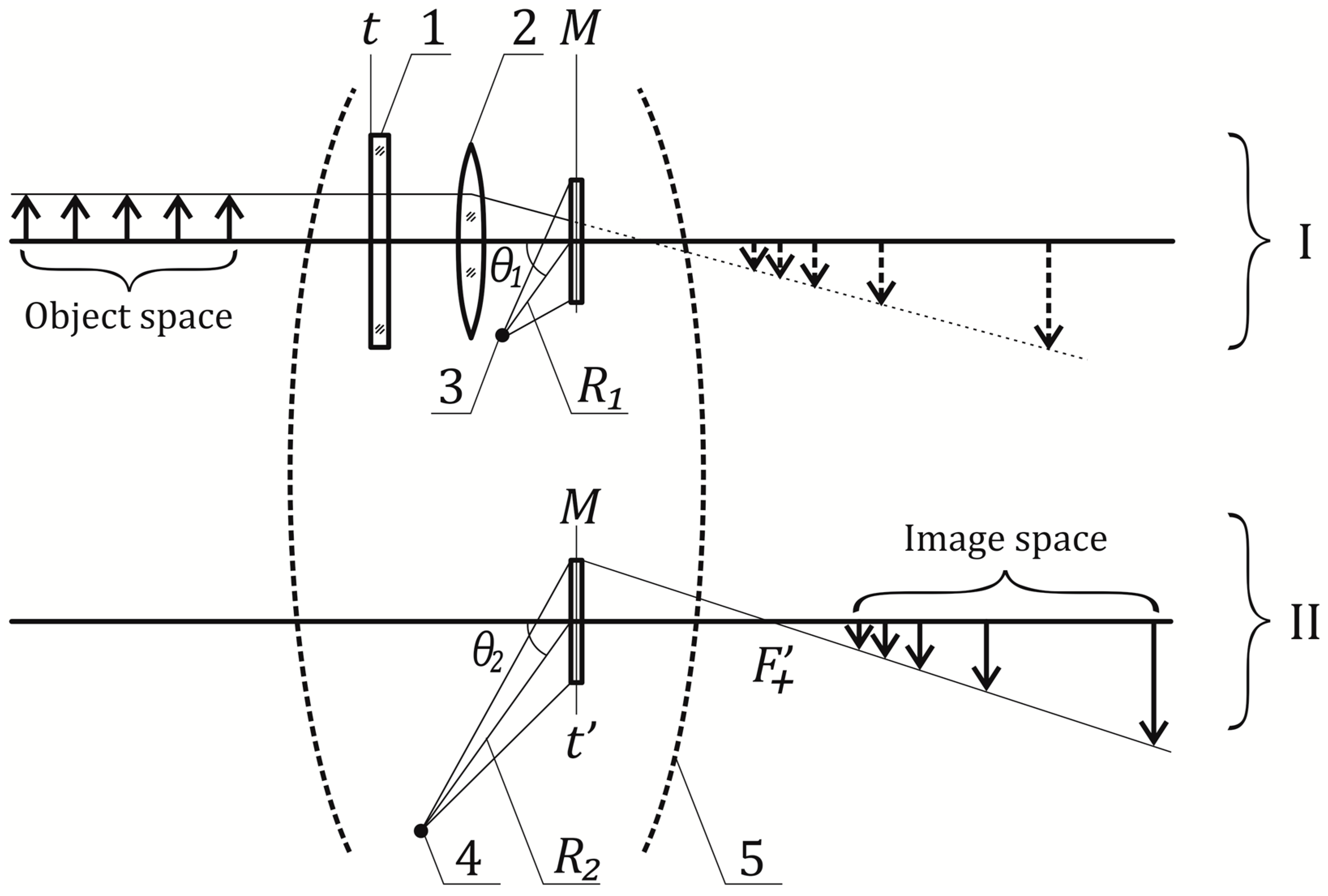
Similar to our studies in [30], we use a generalized equivalent scheme (Figure 2), which includes two stages, to describe the process of obtaining an image of a particle using a digital holographic camera (DHC). At the first stage (I in Figure 2), the lens (2) constructs a real image of particle (or other object), which is considered virtual with respect to the matrix receiver M. It is evident that the lens changes the parameters of both the reference and object waves, and, therefore, the parameters of their interference pattern, which is registered at the matrix receiver and is transmitted to the computer as a two-dimensional array of discrete quantized values of the intensity distribution (digital hologram). The second stage (II in Figure 2) is fully digital, implying the numerical reconstruction of images from a digital hologram [22,23,24,25]. Thus, the equivalent imaging optical system (5, Figure 2) represents a two-stage imaging optical system and implements two processes contributing to the formation of an optical image. The main parameters of this formal optical system, i.e., the equivalent focal length, decentering and magnification, are determined by a set of parameters of a holographic scheme and software for holographic image reconstruction:

• Lens characteristics (2);
• Receiver position—M;
• Radius of curvature of a reference beam—R₁;
• Angle of incidence of a reference beam—θ₁;
• Radiation wavelength at the recording stage—λ₁;
• Radius of curvature of a virtual reconstruction beam—R₂;
• Angle of incidence of a virtual reconstruction beam—θ₂ (does not always coincide with θ₁);
• Virtual radiation wavelength at the reconstruction stage—λ₂.

In our work, we use the most common in-line scheme in the holography of particles (Figure 1), in which the angles θ₁ and θ₂ coincide and equal zero. Further, we will consider particularly this case: θ₁ = θ₂ = 0.

The measurements of geometric parameters and coordinates are performed in a reconstructed holographic image of a particle. The reliable knowledge of the size and position of the studied particle in the space requires the solution of an inverse problem using the measured holographic data as the input data. It is clear that there is a need to calculate the return path of beams through an equivalent optical system. This requires the maximum accurate knowledge of the above parameters of the optical system.

Since the result of holographing and subsequent reconstruction is particle imaging, then it could be argued that a digital holographic system is an imaging optical system. Then, the task of determining the above parameters can be significantly simplified by using the known formulas of geometric optics, in particular Newton’s formula.

On the other hand, this task is complicated by the fact that in a real holographic experiment, the optical parameters of the system do not coincide for various reasons when we record a hologram and reconstruct an image. This may be caused by the use of a projection lens (2) (Figure 2) at the hologram recording stage, the introduction of additional optical elements into the registration scheme (portholes, prisms, calibers), the lack of information on the refractive index of the medium with the particles and, as a result, inaccurate data on the shape of the wavefront (beam divergence) at the hologram recording stage. This means that during the image reconstruction, a digital hologram will serve as another optical system with optical properties depending on the mismatch of system parameters in hologram recording and image reconstruction.

Thus, a new optical system is formed as a result of the composition of two optical systems, whose characteristics are determined by the optical forces of the used components and the distance between them [31]. The optical scheme of such a system is shown in Figure 3, which was previously described in our work [30]. Here, we will consider in more detail the assessment of the error of using an equivalent optical system and the peculiarities of its application in various conditions. In geometric-optical calculation using Newton’s formula [31,32,33,34], the distances in the object space x and the image space x′ are counted from the front and back focal planes, i.e., planes perpendicular to the optical axis in which the front F and back F′ focuses are located, respectively (Figure 3). The object space in the considered natural optical experiment using a submersible digital holographic camera (DHC) represents an aqueous medium with an unknown refractive index with the studied particles, while the position of the focuses, as well as the values of the front f and back f′ focal lengths of the optical system, are unknown. Therefore, let us write formal expressions for an ideal optical system using an arbitrary starting point of distances, both in object and image spaces.

The following are chosen as the reference planes $t$ and $t^{\prime }$ to measure the segments in the equivalent DHC optical scheme: $t$ is the outer surface of a porthole separating the medium with the particles (water) from the medium with the lens and the recording matrix (inner cavity of a camera, air), while $t^{\prime }$coincides with the surface of the recording matrix M (Figure 2). In this case, the segments in the object space are marked in water, while in the image space, they are marked in air. The equivalent optical scheme (Figure 3) is built in such a way that the position of the front focal plane is set by the segment $x_0$ marked from the plane $t$, while in the image space, the plane $t^{\prime }$ is set by the segment ${x_0}^{\prime }$ from the back focal plane. Let ${x^{\prime }}_0^M$ be the segment at which the recording matrix of the camera (plane M) is set from the back focus $F\mathrm{’}$.

Let us consider the case when the position of the i object (particle) with the size $y_i$in the object space is set by the segment $x_i^t$. Then, for the segment $x_i$ setting the position of this object relative to the front focus and for the segment ${x^{\prime }}_i$setting the position of the image plane of the i object relative to the back focus, we can write the ratios obvious from Figure 3:

$$x_i=x_i^t-x_0,$$

(1)

$${x^{\prime }}_i={x^{\prime }}_i^{t^{\prime }}-{x^{\prime }}_0,$$

(2)

where ${x^{\prime }}_i^{t^{\prime }}$—segment setting the position of the image of the i object relative to the plane $t^{\prime }$. The size of this image ${y^{\prime }}_i={\beta }_i·y_i$by determining the magnification ${\beta }_i$ of the optical system.

Following Newton’s formula, we can write

$$x_i·{x^{\prime }}_i=f·f^{\prime }.$$

(3)

Note here that in the general case $f\ne -f^{\prime }$, since there may be different media (water and air, as in the case of the DHC) in the object and image spaces, different optical systems may be used (for example, porthole and prism systems, as in the case of the DHC with a “folded” configuration [1,29]).

For magnification, taking into account (1) and (2), we obtain the following ratios:

$${\beta }_i=-f/x_i=-f/\left(x_i^t-x_0\right),$$

(4)

$${\beta }_i=-{x^{\prime }}_i/f^{\prime }=-\left({x^{\prime }}_i^{t^{\prime }}-{x^{\prime }}_0\right)/f^{\prime }.$$

(5)

By substituting the ratios (1) and (2) into (3), we obtain Newton’s formula for the considered case of random positions of the planes $t$ and $t^{\prime }$, from which the segments in the object and image spaces are set:

$$\left(x_i^t-x_0\right)·\left({x^{\prime }}_i^{t^{\prime }}-{x^{\prime }}_0\right)=f·f^{\prime }.$$

(6)

The ratios (4), (5) and (6) may be used to calibrate the considered optical system equivalent to a digital holographic measuring system. Indeed, they can be used for the ratios of the size $y_i$and the position $x_i^t$ of an arbitrary object:

$$y_i={y^{\prime }}_i/{\beta }_i=-{y^{\prime }}_i·f^{\prime }/\left({x^{\prime }}_i^{t^{\prime }}-{x^{\prime }}_0\right),$$

(7)

$$x_i^t=f·f^{\prime }/\left({x^{\prime }}_i^{t^{\prime }}-{x^{\prime }}_0\right)+x_0.$$

(8)

The simplest method of calibration is the interpolation of dependencies:

$$x^t=x^t\left({x^{\prime }}^{t^{\prime }}\right) \mathrm{and} \beta =\beta \left({x^{\prime }}^{t^{\prime }}\right).$$

(9)

The exact view of the interpolation polynomial from (8) to describe the dependency $x^t\left({x^{\prime }}^{t^{\prime }}\right)$ is written as follows:

$$x^t\left({x^{\prime }}^{t^{\prime }}\right)=A+B/\left({x^{\prime }}^{t^{\prime }}-C\right).$$

(10)

From the Formula (7), we obtain the exact kind of interpolation polynomial to describe the dependency $\beta \left({x^{\prime }}^{t^{\prime }}\right)$:

$$\beta \left({x^{\prime }}^{t^{\prime }}\right)=-\left({x^{\prime }}^{t^{\prime }}-C\right)/D,$$

(11)

where $A,B,C,D$—some coefficients.

While determining the coefficients $A,B,C,D$ based on a digital holographic experiment, the difference in the shape of the recording and reconstruction beams will be automatically taken into account, and thus, there will be no need to know the refractive index of the medium in which the particles are located. This significantly increases the reliability of the measured parameters, since it is obvious that when we use a lens (for example, in the DHC), a converging reference beam with unknown convergence is used during recording, while the flat one is used in numerical reproduction for ease of calculation. In fact, expressions (10) and (11) represent a mathematical model using a well-developed geometric optics apparatus. Such a mathematical model establishes the desired one-to-one correspondence between the digital holographic image of a particle and the holographing (displaying) particle itself.

The task of finding coefficients is solved by calibration in both laboratory and real conditions. For calibration, we use test particles in the form of opaque squares with a side of 500 μm, placed photolithographically on a glass plate with a thickness of 2.65 mm (calibers, Figure 4a). The DHC design provides the fixation of four calibers (Figure 4b). The positions of the test particles in the object space are set structurally by segments $x_1^t, { x}_2^t, { x}_3^t, x_4^t$ from the reference position $t$ coinciding with the outer surface of a submersible DHC porthole (Figure 2 and Figure 3). The sizes of test particles are $y_1={ y}_2=y_3={ y}_4=$ 500 µm, and thus the increase in the optical system for these particles will be ${\beta }_1, {\beta }_2, { \beta }_3, { \beta }_4$, respectively. If a hologram of four test particles is recorded on a matrix, then the sizes ${y^{\prime }}_1, {y^{\prime }}_2, {y^{\prime }}_3, {y^{\prime }}_4$of the images of particles reconstructed from digital holograms and distances ${x^{\prime }}_1^{t^{\prime }}, {x^{\prime }}_2^{t^{\prime }}, {x^{\prime }}_3^{t^{\prime }},{x^{\prime }}_4^{t^{\prime }}$ from the reference point $t^{\prime }$ coinciding with plane M of the digital hologram recording to these images will be defined during numerical reconstruction. When reconstructing the holographic image shown in Figure 4c, a spatial frequency method was used to suppress the twin-image effect [35].

In real experiments, the refractive indices of the medium where the studied particles (fresh water, sea water or air) are located differ from the refractive index of the glass, so it is necessary to take into account the refractive index of the medium $n_{wg}$ relative to the glass of the calibers and prisms. Note that the portholes are not included in the studied volume. The segments in the space of objects are counted from the first surface of a porthole of the recording unit (point O, Figure 3), so they are simply included in the optical system. Then,

$$x^t=x_w^t-x_g^t(n_{gw}-1),$$

(12)

where $x_w^t$—geometric coordinate of the particle in the medium, $x_g^t$—thickness of the optical elements of the working volume. Let us define $n_{gw}$ with coefficient $E$, then the expression (10) will be as follows:

$$x_w^t-x_g^t(E-1)=A+B/\left({x^{\prime }}^{t^{\prime }}-C\right),$$

(13)

Thus, in order to determine the calibration coefficients $A,B,C,D, E$ for the considered digital holographic system, it is necessary to solve the following system of nonlinear equations:

$$\left\{\begin{array}{c}{x_1}_w^t-{x_1}_g^t(E-1)=A+\frac{B}{{{x_1}^{\prime }}^{t^{\prime }}-C}\\ {x_2}_w^t-{x_2}_g^t(E-1)=A+\frac{B}{{{x_2}^{\prime }}^{t^{\prime }}-C}\\ {x_3}_w^t-{x_3}_g^t(E-1)=A+\frac{B}{{{x_3}^{\prime }}^{t^{\prime }}-C}\\ {x_4}_w^t-{x_4}_g^t(E-1)=A+\frac{B}{{{x_4}^{\prime }}^{t^{\prime }}-C}\\ y_1=-\frac{{y^{\prime }}_1·D}{{x^{\prime }}_1^{t^{\prime }}-C }\end{array}\right.$$

(14)

Of the first four equations of the system (14), one of the numerical methods can be used to find a solution for coefficients $A,B,C,E$. The last equation in (14) allows us to define the coefficient $D$ by using the found value C. In this case, as the system shows (14), four calibration measurements are used, i.e., there is no need for a fifth caliber. Thus, the optimal number of calibration measurements is 4, and they can be performed by a simultaneous recording of four calibers per one hologram. To do that, 4 calibers are placed in the beam illuminating the studied volume of the medium with particles (Figure 4b). Such calibration does not require reliable knowledge of the optical properties of the components and media (in this case water, glass and air) included in the equivalent optical scheme. At the same time, based on the change in the calibration coefficients, it is possible to detect a change in the optical properties of the medium where the measurements are made.

Indeed, coefficients $A,B,C,D,E$—values with apparent optical interpretation:

• $A=x_0$—segment set from the front focal plane, which specifies the position of the reference point in the object space (plane $t$);
• $B=f·f^{\prime }$—product of the front $f$ and back $f^{\prime }$ focal lengths of the equivalent optical system;
• $C={x^{\prime }}_0$—segment set from the back focal plane, which specifies the position of the reference point in the image space (plane $t^{\prime }$);
• $D=f^{\prime }$—value of the back focal length of the optical system;
• $E=n_{gw}$—refractive index of the medium relative to the glass of calibers and prisms.

After finding coefficients $A,B,C,D, E$, it is possible to determine the position and size of particles, using expressions (11) and (13). These measurements are indirect, and the relevant values represent the functions of the measured values ${x^{\prime }}^{t^{\prime }}$ and $y^{\prime }$:

$$x_w^t\left({x^{\prime }}^{t^{\prime }}\right)=x_g^t\left(E-1\right)+A+B/\left({x^{\prime }}^{t^{\prime }}-C\right),$$

(15)

$$y\left({x^{\prime }}^{t^{\prime }}, y^{\prime }\right)=-y^{\prime }·D/\left({x^{\prime }}^{t^{\prime }}-C\right).$$

(16)

Since the images of the volume cross-sections are reconstructed from a hologram at a fixed pitch along the longitudinal coordinate and the transverse coordinates and dimensions are also determined discretely, there is an error in determining the coordinates and sizes of particles. The error associated with such sampling in the measurement of ${x^{\prime }}^{t^{\prime }}$ and $y^{\prime }$ is defined as follows:

$$\delta x_w^t=\pm \left|\partial x_w^t/\partial {x^{\prime }}^{t^{\prime }}\right|\delta {x^{\prime }}^{t^{\prime }}=\pm \left|B/{\left({x^{\prime }}^{t^{\prime }}-C\right)}^2\right|\delta {x^{\prime }}^{t^{\prime }},$$

(17)

$$\delta y=\pm \left[\left|\partial y/\partial {x^{\prime }}^{t^{\prime }}\right|\delta {x^{\prime }}^{t^{\prime }}+\left|\partial y/\partial y^{\prime }\right|\delta y^{\prime }\right]=\pm \left[\left|y^{\prime }·D/{\left({x^{\prime }}^{t^{\prime }}-C\right)}^2\right|\delta {x^{\prime }}^{t^{\prime }}+\left|D/\left({x^{\prime }}^{t^{\prime }}-C\right)\right|\delta y^{\prime }\right],$$

(18)

where $\partial x_w^t/\partial {x^{\prime }}^{t^{\prime }}$, $\partial y/\partial {x^{\prime }}^{t^{\prime }}$, $\partial y/\partial y^{\prime }$—partial derivatives $x_w^t\left({x^{\prime }}^{t^{\prime }}\right)$ and $y\left({x^{\prime }}^{t^{\prime }}, y^{\prime }\right)$ according to arguments ${x^{\prime }}^{t^{\prime }}$ and $y^{\prime }$, and $\delta {x^{\prime }}^{t^{\prime }}$ and $\delta y^{\prime }$—sampling interval (pitch) during reconstruction. To find a random error of indirect measurements, the following formulas can be used:

$$∆x_w^t=\pm \sqrt{{\left(\left|\partial x_w^t/\partial {x^{\prime }}^{t^{\prime }}\right|∆{x^{\prime }}^{t^{\prime }}\right)}^2}=\pm \left(B/{\left({x^{\prime }}^{t^{\prime }}-C\right)}^2\right)∆{x^{\prime }}^{t^{\prime }}.$$

(19)

$$∆y=\pm \sqrt{{\left(\left|\partial y/\partial {x^{\prime }}^{t^{\prime }}\right|∆{x^{\prime }}^{t^{\prime }}\right)}^2+{\left(\left|\partial y/\partial y^{\prime }\right|{∆y}^{\prime }\right)}^2}=\pm \sqrt{{\left(y^{\prime }·D·∆{x^{\prime }}^{t^{\prime }}/{\left({x^{\prime }}^{t^{\prime }}-C\right)}^2 \right)}^2+{\left(D·∆y^{\prime }/\left({x^{\prime }}^{t^{\prime }}-C\right)\right)}^2},$$

(20)

where $∆{x^{\prime }}^{t^{\prime }}$ and $∆y^{\prime }$—confidence intervals at given confidence probabilities for arguments ${x^{\prime }}^{t^{\prime }}$ and $y^{\prime }$. It should noted that the confidence intervals $∆{x^{\prime }}^{t^{\prime }}$ and $∆y^{\prime }$ should be taken with the same confidence probability $p$, then the reliability for the confidence interval $∆y^{\prime }$ will also be $p$.

The estimates of the total error of measurement results:

$$∆\overline{x_w^t}=\sqrt{{\left(∆x_w^t\right)}^2+{\left(\delta x_w^t\right)}^2}$$

(21)

$$∆\overline{y}=\pm \sqrt{{\left(∆y\right)}^2+{\left(\delta y\right)}^2}$$

(22)

In this paper, all confidence intervals are taken with the same confidence probability $p$ = 95%. The average values measured during calibration were calculated based on ten measurements.

3. Results

This paper presents the results of calibration experiments performed in both field and laboratory conditions. The results of field experiments were obtained during two expeditions to study plankton using a digital holographic camera: in the Arctic in October 2020 and on Lake Baikal in February 2022 (51°53′54.42″ N 105°03′53.46″ E). During the Arctic expedition, the digital holograms of calibers (a square of $y_c=500$ µm on side) were recorded by submerging in sea water at three stations—No. 6935 (74°22′57.2″ N 72°53′04.3″ E) in the Kara Sea (Ob river estuary) on 2 October 2020, No. 6939 (77°17′04.4″ N 122°05′44.7″ E) on 6 October 2020 and No. 6952 (76°53′29.4″ N 127°47′34.8″ E) in the Laptev Sea on 9 October 2020. In laboratory conditions, the calibers were registered both in the air and with the camera submerged in fresh water.

The holograms of calibers were recorded when the DHC was submerged at different depths during field calibration experiments. Digital holograms are recorded using radiation with a wavelength of 650 nm and a CMOS camera with a frame size of 2048 × 2048 pixels and a pixel size of 3.45 µm. The diameter of the illuminated area is 35 mm, and the size of the field of view is determined by the shape of the matrix and makes 24.7 × 24.7 mm. The positions of the planes of the best (most focused) caliber images ${x^{\prime }}_1^{t^{\prime }}=\overline{{x^{\prime }}_1^M}, {x^{\prime }}_2^{t^{\prime }}=\overline{{x^{\prime }}_2^M}, {x^{\prime }}_3^{t^{\prime }}=\overline{{x^{\prime }}_3^M}, {x^{\prime }}_4^{t^{\prime }}=\overline{{x^{\prime }}_4^M}$in relation to the position of a matrix and the size (square side) of a caliber $\overline{{y^{\prime }}_1}$ were determined from the reconstructed images of calibers (

Table 1. Results of the DHC calibration under various conditions.

Station	No. 6935, Kara Sea, 2 October 2020	No. 6939, Laptev Sea, 6 October 2020	No. 6952, Laptev Sea, 9 October 2020	Laboratory, without Water	Laboratory, Fresh Water	Lake Baikal, 18 February 2022
$\overline{{x^{\prime }}_1^M}\pm ∆\overline{{x^{\prime }}_1^M}$, mm	52.8 ± 0.1	52.9 ± 0.1	52.8 ± 0.1	55.2 ± 0.1	52.5 ± 0.2	44.9 ± 0.1
$\overline{{x^{\prime }}_2^M}\pm ∆\overline{{x^{\prime }}_2^M}$, mm	72.0 ± 0.1	72.4 ± 0.1	72.5 ± 0.1	79.9 ± 0.1	70.9 ± 0.2	61.6 ± 0.4
$\overline{{x^{\prime }}_3^M}\pm ∆\overline{{x^{\prime }}_3^M}$, mm	168.2 ± 0.2	170.1 ± 0.3	170.8 ± 0.5	182.7 ± 0.3	160.1 ± 0.4	171.4 ± 0.7
$\overline{{x^{\prime }}_4^M}\pm ∆\overline{{x^{\prime }}_4^M}$, mm	189 ± 2	190.3 ± 0.5	189.1 ± 0.7	209.1 ± 0.3	183 ± 1	202.7 ± 0.9
$\overline{{y\mathrm{’}}_1}\pm ∆\overline{{y\mathrm{’}}_1}$, µm	229 ± 4	231 ± 4	231 ± 4	227 ± 4	220 ± 4	205 ± 4
$A$	5947	7356	16,971	5376	3609	1759
$B$	−5,331,085	−8,340,704	−45,588,774	−5,618,777	−1,839,368	−602,189
$C$	−852	−1090	−2642	−1001	−465	−309
$D$	−1976	−2473	−5834	−2326	−1176	−863
$E$	1.30	1.26	1.16	1.61	1.48	1.50

). The position of the best image plane of particles was determined visually by an operator according to the best image sharpness. The image size (square side) of the caliber test particle was determined by counting the number of pixels along the image side and multiplying by the pixel size of the used digital camera (3.45 µm). Indeed, to calculate the field distribution in the reconstructed images, we use the convolution method [22,23,24,25]. In this case, the pixel size in the hologram (camera) is equal to the pixel size in the image [22,23]; there is no scaling, and therefore, we use the pixel size of the camera. Then, by calibration, we find the magnification factor $\beta$ (Formula (11)) of the equivalent optical system, i.e., we can define the actual pixel size in the image. The mean values ${x^{\prime }}_i^M$and $\overline{{y^{\prime }}_1}$ are calculated from ten measurements (ten digital holograms recorded at different depths were used). In this case, $\delta {x^{\prime }}^{t^{\prime }}=$ 0.1 mm (pitch of the reconstruction of the images of sections of the registered volume from a digital hologram) and $\delta y^{\prime }=$ 3.45 µm (pixel size of the recording camera). Table 1 shows the total measurement error $∆\overline{{x^{\prime }}_i^M}$and $∆\overline{{y\mathrm{’}}_i}$, calculated using Formulas (21) and (22).

In the described field experiments, we used the DHC with an in-line scheme but with a “folded” configuration of the working volume, which has small-sized unit compared to a linear in-line holographic scheme. The prisms ensured the four passes of the working volume with a laser beam (2, Figure 5).

The calibers (3) were located in the registered volume of the DHC in positions determined by the segments (Figure 5) defined at the design stage: ${x_1}_w^t=r_1=57.5$ mm, ${x_1}_g^t=0$, ${x_2}_w^t=r_1+{d+r}_2=180.65$ mm, ${x_2}_g^t=d=2.65$ mm, ${x_3}_w^t=r_1+{2d+r}_2+2r_3+3l+2r_4=816.3$ mm, ${x_3}_g^t=2d+3l=305.3$ mm, ${x_4}_w^t=r_1+{3d+2r}_2+2r_3+3l+2r_4=921.45$ mm and ${x_4}_g^t=3d+3l=307.95$ mm. Here, $d$—thickness of the caliber glass plate and $l$—path traveled by the beam in the prism. Note that the DHC configuration in the expedition on Lake Baikal was different in the size of the studied volume and location of calibers: ${x_1}_w^t=57.5$ mm, ${x_2}_w^t=135.5$ mm, ${x_3}_w^t=658.35$ mm and ${x_4}_w^t=736.35$ mm.

To solve the system of nonlinear Equation (14), the Levenberg–Marquardt algorithm [36,37] was applied, and the values $\overline{{x^{\prime }}_i^M}$ and $\overline{{y\mathrm{’}}_1}$ averaged over ten holograms were used. The results are shown in Table 1.

Thus, using the obtained coefficients A, B, C, D, the expressions (16) and (17) and data (coordinates and size) obtained from reconstructed holographic images of particles, it is possible to determine the true coordinates of the particle and its size.

As an example, Figure 4c shows a digital hologram of calibers recorded at station No. 6939 (Laptev Sea) at a depth of 24.91 m and the reconstructed images of test caliber particles (1–4) and plankton particles (5–6). The size $y_i$of test and plankton particles, taking into account the coefficients $A,B,C,D, E$ from Table 1 for a given station, were adjusted according to Formula (16) and reflected in

Table 2. Size and position of particles, whose reconstructed images are shown in Figure 4b, recorded at station No. 6939, determined without taking into account coefficients $A,B,C,D, E$ (${y^{\prime }}_i$ and ${x^{\prime }}_i^{t^{\prime }}$, respectively) and corrected with respect to coefficients $A,B,C,D, E$ from Table 1 ($y_i$ and ${x_i}_w^t$, respectively). The error (%) is shown in parentheses.

For i Particle in Figure 4	1st Caliber	2nd Caliber	3rd Caliber	4th Caliber	Plankton Particle (5, Figure 4)	Plankton Particle (6, Figure 4)
${x^{\prime }}_i^{t^{\prime }}\pm \Delta {x^{\prime }}_i^{t^{\prime }}$, obtained for the station No. 6939 ($\left(\left|{x^{\prime }}_i^{t^{\prime }}-{x_i}_w^t\right|/{x_i}_w^t\right)·100$, %)	52.9 ± 0.1 mm (8%)	72.4 ± 0.1 mm (59.9%)	170.1 ± 0.3 mm (79.2%)	190.3 ± 0.5 mm (79.3%)	181.2 mm	183.7 mm
${x_i}_{w\left(6939\right)}^t\pm ∆\overline{{x_i}_{w\left(6939\right)}^t}$ considering coefficients obtained at the station No. 6939 ($\left(∆\overline{{x_i}_{w\left(6939\right)}^t}/{x_i}_{w\left(6939\right)}^t\right)·100$, %)	57.5 ± 0.8 mm (1.4%)	180.7 ± 0.9 mm (0.5%)	816 ± 2 mm (0.2%)	921 ± 2 mm (0.3%)	876 ± 2 mm	890 ± 2 mm
${x_i}_{w\left(water\right)}^t\pm ∆\overline{{x_i}_{w\left(water\right)}^t}$ considering coefficients obtained in laboratory conditions in water ($\left(\left|{x_i}_{w\left(water\right)}^t-{x_i}_{w\left(6939\right)}^t\right|/{x_i}_{w\left(6939\right)}^t\right)·100$, %)	60.2 ± 0.8 mm (4.7%)	190.2 ± 0.9 mm (5.3%)	862 ± 1 mm (5.6%)	953 ± 2 mm (3.8%)	914 ± 2 mm (4.3%)	925 ± 2 mm (3.9%)
${x_i}_{w\left(6935\right)}^t\pm ∆\overline{{x_i}_{w\left(6935\right)}^t}$ considering coefficients obtained at the station No. 6935 ($\left(\left|{x_i}_{w\left(6935\right)}^t-{x_i}_{w\left(6939\right)}^t\right|/{x_i}_{w\left(6939\right)}^t\right)·100$, %)	58.2 ± 0.8 mm (1.2%)	183.7 ± 0.9 mm (1.7%)	826 ± 2 mm (1.2%)	928 ± 3 mm (0.8%)	883 ± 2 mm (0.8%)	895 ± 2 mm (0.6%)
${x_i}_{w\left(6952\right)}^t\pm ∆\overline{{x_i}_{w\left(6952\right)}^t}$ considering coefficients obtained at the station No. 6952 ($\left(\left|{x_i}_{w\left(6952\right)}^t-{x_i}_{w\left(6939\right)}^t\right|/{x_i}_{w\left(6939\right)}^t\right)·100$, %)	58.1 ± 0.8 mm (1%)	182.2 ± 0.9 mm (0.8%)	812 ± 2 mm (0.5%)	921 ± 3 mm (0%)	876 ± 2 mm (0%)	891 ± 2 mm (0.1%)
${y^{\prime }}_i\pm ∆\overline{{y\mathrm{’}}_i}$, considering coefficients obtained at the station No. 6939 ($\left(\left|{y^{\prime }}_i-y_c\right|/y_c\right)·100$, %)	231 ± 4 µm (53.8%)	232 ± 4 µm (53.6%)	231 ± 4 µm (53.8%)	231 ± 4 µm (53.8%)	424.35 µm	376.05 µm
$y_{i\left(6939\right)}\pm ∆\overline{y_{i\left(6939\right)}}$ considering coefficients obtained at the station No. 6939 ($\left(\left|y_{i\left(6939\right)}-y_c\right|/y_c\right)·100$, %)	500 ± 8 µm (0%)	498 ± 8 µm (0.4%)	489 ± 7 µm (2.2%)	486 ± 7 µm (2.8%)	893 ± 7 µm	791 ± 7 µm
$y_{i\left(water\right)}\pm ∆\overline{y_{i\left(water\right)}}$ considering coefficients obtained in laboratory conditions in water ($\left(\left|y_{i\left(water\right)}-y_{i\left(6939\right)}\right|/y_{i\left(6939\right)}\right)·100$, %)	525 ± 8 µm (5%)	506 ± 8 µm (1.2%)	430 ± 8 µm (14%)	415 ± 8 µm (17%)	772 ± 8 µm (6.4%)	682 ± 8 µm (8.7%)
$y_{i\left(6935\right)}\pm ∆\overline{y_{i\left(6935\right)}}$ considering coefficients obtained at the station No. 6935 ($\left(\left|y_{i\left(6935\right)}-y_{i\left(6939\right)}\right|/y_{i\left(6939\right)}\right)·100$, %)	504 ± 8 µm (0.8%)	494 ± 8 µm (1.2%)	448 ± 8 µm (10.4%)	439 ± 8 µm (12.2%)	811 ± 8 µm (1.7%)	717 ± 8 µm (1.8%)
$y_{i\left(6952\right)}\pm ∆\overline{y_{i\left(6952\right)}}$ considering coefficients obtained at the station No. 6952 ($\left(\left|y_{i\left(69352\right)}-y_{i\left(6939\right)}\right|/y_{i\left(6939\right)}\right)·100$, %)	498 ± 8 µm (0.4%)	496 ± 8 µm (0.8%)	481 ± 8 µm (3.8%)	476 ± 8 µm (4.8%)	877 ± 8 µm (1.7%)	776 ± 8 µm (1.8%)

. The position ${x_i}_w^t$of particles was calculated using Formula (15). The total errors $∆\overline{{x_i}_w^t}$ and $∆\overline{y_i}$ were determined by Formulas (21) and (22), respectively.

For comparison, Table 2 also shows the calculation of size and position of particles recorded at station No. 6939 using coefficients $A,B,C,D, E$ obtained at other stations and in laboratory conditions in fresh water. The relative error is shown in parentheses.

Table 3. Size and position of calibers determined without coefficients $A,B,C,D,E$ (${y^{\prime }}_i$and ${x^{\prime }}_i^{t\prime }$, respectively) and corrected with regard to coefficients $A,B,C,D,E$ from Table 1 ($y_i$and $x_{wi}^t$, respectively) for the station at Lake Baikal. The error (%) is shown in parentheses.

For i Particle in Figure 4	1st Caliber	2nd Caliber	3rd Caliber	4th Caliber
${x^{\prime }}_i^{t^{\prime }}\pm \Delta \overline{{x^{\prime }}_i^{t^{\prime }}}$, mm	44.9 ± 0.1 (21.9%)	61.6 ± 0.4 (54.5%)	171.4 ± 0.7 (52.2%)	202.7 ± 0.9 (53.5%)
${x_i}_w^t\pm ∆\overline{{x_i}_w^t}$, mm	57.5 ± 0.6 (1%)	136 ± 2 (1.5%)	658 ± 2 (0.3%)	736 ± 2 (0.3%)
${y^{\prime }}_i\pm ∆\overline{{y\mathrm{’}}_i}$, µm	205 ± 4 (59%)	214 ± 4 (57.2%)	278 ± 5 (44.4%)	287 ± 8 (42.6%)
$y_i\pm ∆\overline{y_i}$, µm	500 ± 9 (1.8%)	498 ± 8 (1.6%)	500 ± 7 (1.4%)	484 ± 10 (3.2%)

shows the size $y_i$ and position $x_{wi}^t$of corrected test particles, taking into account coefficients $A,B,C,D,E$ from Table 1 for the station at Lake Baikal.

4. Discussion

Coefficients $A,B,C,D$ characterize the equivalent optical system of the DHC camera taking into account the medium in which holograms are recorded. An equivalent DHC optical scheme shown in Figure 6 can be built for the station No. 6939 in the Laptev Sea.

Note that the obtained results (Table 1) show that the coefficient $E$ for the experiment without water, in fresh and in sea water (stations No. 6935 and No. 6939), is different, which indicates a different refractive index of the media in which the holograms were recorded. If necessary, this can be used to detect the difference in optical (and, therefore, hydrophysical) properties of media without the use of additional measuring tools.

The large values of coefficients A, D, C are explained by the fact that the equivalent scheme is an almost afocal system that converts a parallel light beam into a parallel one. The word “almost” here means the uncertainty associated with the divergence of the reference beam during hologram recording. Therefore, the error in determining the longitudinal coordinates may strongly be affected by the error in the applied calculation methods and the inaccuracy of estimating the values of parameters. Formulas (17), (19) and (21) show that the total error in defining the position of particle $∆\overline{x_w^t}$ depends on the position of particle ${x^{\prime }}^{t^{\prime }}$, defined through a holographic experiment and the error value of its definition $∆{x^{\prime }}^{t^{\prime }}$. A random error $∆x_w^t$ contributes the most to the total error $∆\overline{x_w^t}$. In turn, the error of measuring the longitudinal coordinates of particles based on images reconstructed from digital holograms $∆x_w^t$increases with an increase in the distance from a hologram to an image of a particle numerically reconstructed from it [27].

The total error in determining the size of a particle $∆\overline{y}$has more complex dependence (Formulas (18), (20) and (22)) in comparison with $∆\overline{x_w^t}$, and depends on the following values determined from a holographic experiment: particle position ${x^{\prime }}^{t^{\prime }}$and its error $∆{x^{\prime }}^{t^{\prime }}$ and particle size $y^{\prime }$ and its error ${∆y}^{\prime }$. The minimum value $∆\overline{y}$ = 7 μm is determined by a sampling error $\delta y^{\prime }=$ 3.45 μm, which is the pixel size of the recording camera. It is possible to reduce the error in determining the particle size by replacing it with a smaller-pixel camera or by using numerical methods to increase the resolution of an image reconstructed from a digital hologram [38,39,40,41].

Let us consider the data obtained on Lake Baikal (Table 3). The error in determining the position of a particle does not exceed 1.5%, and the error in determining the particle size is 3.2%. The values of the coefficient $E$ (Table 1), which determines the refractive index of the medium $n_{wg}$ relative to the glass of calibers and prisms, are quite close for stations in Lake Baikal and measurements in laboratory fresh water within the measurement error ($E=$ 1.48 ± 0.05 for fresh water, $E=$ 1.50 ± 0.05 for Lake Baikal). This confirms the fact that the results of calibration performed in fresh water in the laboratory can be used for the experiments in Lake Baikal, where the water is also fresh.

The computational experiment in Table 2 shows that if we use the coefficients $A,B,C,D,E$ obtained during fresh water calibration to determine the size and position of particles recorded in sea water (station No. 6939), the error in determining the position of particles increases to 5.6%, and the size to 17%. The error in determining the size and position of particles when we use the calibration results in water areas of different seas is also quite high. When we use the coefficients obtained at station No. 6935 to determine the parameters of particles recorded at station No. 6939, the error in determining the position of particles increases to 1.7%, and the size to 12.2%. The calibration experiment in the water area of the same sea at stations No. 6939 and No. 6952 (Laptev Sea) shows that the error in determining the position of particles does not exceed 1%, and the size of particles does not exceed 4.8%. Thus, it may be concluded that calibration should be performed in each water area with one calibration experiment, the results of which can be further applied to all stations of this water area. An important condition for the use of calibration for different stations in the same water area is the same refractive index of the medium (or the conductivity of water). Calibration can be performed in laboratory conditions, but the salt composition of water in the laboratory must correspond to the composition of water used in the marine experiment.

5. Conclusions

The paper presents an equivalent optical imaging system of a digital holographic camera for recording particles. This equivalent scheme made it possible to build a mathematical model for the in-line scheme that establishes a one-to-one correspondence between the dimensional and spatial parameters of the particle digital holographic image and the displaying particles itself. The model coefficients to determine the real size and longitudinal coordinate of a particle based on its holographic image are found by calibration. Field experiments confirmed that the optimal number of calibration measurements to determine the model coefficients (calibers used in simultaneous holographing per one hologram) is four. This does not require data on the optical properties of the components and media (in this case, water, glass and air) included in the equivalent optical scheme. In addition, based on the change in the calibration coefficients, it is possible to detect a change in the optical properties of the medium where the measurements are made.

The developed mathematical model clearly demonstrates that an error in determining the position of a particle does not exceed 1.5%, and its size does not exceed 4.8%. Failure to consider the developed model leads to errors in determining the size of particles (59%) and the position of particles (54.5%) for the case of fresh water. For marine experiments, the failure to consider the model leads to errors (53.8% in terms of particle size and 79.3% in terms of coordinates).

The experiments in field and laboratory conditions showed that for the developed mathematical model, one calibration is quite sufficient within the same water area, since the error in determining the position and size of particles in different places and depths of the water area changes slightly. Calibration may be performed in laboratory conditions, but the salt composition and optical parameters of laboratory water must correspond to the parameters of water in the natural experiment.