Simulation and Experimental Research of V-Crack Testing of Rail Surfaces Based on Laser Ultrasound

Abstract

Rail surface cracks are widespread damage that can lead to uneven surfaces of railheads and affect traveling safety. Non-destructive testing is needed to inspect rails regularly to ensure the normal operation of railroads. This paper proposes a laser ultrasonic testing method combining variational mode decomposition and diffractive Rayleigh wave time-of-flight to detect tiny cracks on the rail surface quantitatively. The finite element method was combined with experiments to simulate and experimentally investigate cracks of different sizes numerically. In the numerical simulation, the location of the crack was determined by B-scan. Afterward, the interaction between various types of ultrasound and cracks was comparatively analyzed, and the crack size was quantitatively characterized using useful information from the ultrasound signals. The results show that the time-of-flight method can detect arbitrary cracks with low error. Therefore, the experimentally acquired ultrasound signals used the time difference between the diffracted Rayleigh wave and other ultrasound waves to detect the crack information quantitatively. The variational mode decomposition method was used to separate the ultrasonic signals and extract the best surface wave modes to improve the signal-to-noise ratio. The results show that the combination of variational mode decomposition and time-of-flight method can effectively detect the size of cracks.

1. Introduction

When a rail is under excessive load pressure for a long time, there will be cracks and other defects in the rail’s head, belly, and foot. As time passes, the cracks that accumulate on the surface of the rail would grow and form transverse defects. When its size reaches a critical level, it can affect the use of the rail and cause the rail to break. Thus, it is essential to find suitable rail detection methods to ensure the safe operation of the rail [1,2].

Ultrasonic testing (UT) and electromagnetic testing (ET) are the most commonly used methods for detecting rail defects [3,4]. Common ET methods include eddy current testing (ECT) and magnetic flux leakage testing (MFL). The principle of ECT is to apply an alternating current to the coil, which induces eddy currents in the specimen. When defects are present, the distribution of the eddy currents changes, leading to a change in the coil’s impedance. Therefore, defects can be detected by measuring changes in the coil’s impedance [5]. However, ECT is susceptible to lift-off effects, which may cause defect signals to be masked by background magnetic field noise [4]. The principle of MFL is to magnetize the specimen. When the magnetic flux inside the specimen encounters a defect, it changes and creates a leakage field, which a sensor can measure. However, various factors (such as magnetization conditions, speed, and lift-off) can interfere with the MFL signal [6].

UT has two detection methods. One is contact detection, which typically uses a contact transducer to receive the ultrasound signal. This method directly contacts the measured object and has good acoustic coupling characteristics. The detection data is stable with minimal noise interference, resulting in high reliability [7]. However, using contact transducers requires couplers, which results in limited detection coverage and makes it unsuitable for detecting certain objects [8].

The other method is non-contact detection, such as phased array ultrasonic testing (PAUT) and laser ultrasound testing (LUT). PAUT uses an array of multiple transducers, each receiving ultrasonic signals from within the material and generating a focused beam by controlling the phase and timing of the signals. This method enables scanning and imaging at various depths and directions [9]. Kim et al. developed a PAUT system to detect rail cracks. The system can evaluate crack sizes larger than 2 mm [10]. Gao et al. used a fiber-optic picosecond laser to detect cracks in steel blocks as an excitation source for PAUT. The data show that the phased-array laser source significantly improves the amplitude and signal-to-noise rate of the diffracted signals compared to a single laser source [11]. LUT can detect internal, surface, and sub-surface defects of complex shapes in hazardous environments [12,13]. Pathak et al. detected rail foot cracks using laser-induced guided waves and simulated the effect of different frequencies and sensor locations on the detection results. This study helps to determine the equipment specifications and sensor locations for rail foot crack detection [14]. LUT can excite multiple ultrasonic wave modes in the measured object, with frequencies reaching the MHz range [15]. Detecting rail surface defects requires high accuracy, so studying LUT technology for detecting rail surface defects is valuable.

However, quantitative detection of rail defects in thermoelastic mode is challenging. This is because of the low energy of the laser-excited body wave, which results in weak diffraction signals and a low signal-to-noise ratio for defect detection [16]. This requires a signal processing technique to improve the signal-to-noise ratio of the ultrasound signal. Commonly used methods include wavelet transform, empirical mode decomposition (EMD), and variational mode decomposition (VMD). Among them, selecting wavelet basis functions is difficult, and EMD can lead to modal aliasing [17,18]. VMD does not require preset basis or wavelet functions, allowing for adaptive signal decomposition. It effectively separates modes and avoids mode overlapping [19]. Based on the advantages mentioned, this paper uses VMD to process ultrasound signals.

Before experimental validation, numerical simulations using the finite element method (FEM) can provide a better understanding of the physical process in LUT. FEM can flexibly handle complex geometrical models and even anisotropic materials. Simulation results can be evaluated quickly and efficiently, reducing expensive and time-consuming experimental costs [20]. Zhu et al. used the difference between phase velocities predicted by a FEM and measured by an array of sensors mounted on the rail to determine the material elastic constants of the rail. The selected waveguide modes, which are sensitive to modulus and insensitive to rail profile changes, can be evaluated for worn rails [21]. Wang et al. used the FEM to simulate a variety of ultrasonic signal patterns and responses to metal defects. The results show that the variation of Rayleigh and shear waves can detect surface cracks and internal defects in specimens [22]. On this basis, Han et al. fitted different modes of the ultrasonic signal with the crack size to complete the characterization of surface oblique cracks [23].

Existing research on rail defect detection is predominantly focused on qualitative methods. However, qualitative detection does not provide specific defect data and may fail to accurately assess the severity of defects, potentially overlooking severe issues. This paper establishes a numerical model based on the FEM for using laser-excited ultrasonic waves in rails. The crack size was quantitatively characterized using pulse-echo, pitch-catch, and time-of-flight (TOF) methods. The method with the best detection effect and the slightest error is selected based on the characterization results to guide the subsequent experiments. After that, the simulation results are verified using a LUT system. A VMD algorithm with a low signal-to-noise ratio is used for the ultrasonic signals to obtain the optimal ultrasonic wave modes. The angle, depth, and width of the V-shaped cracks on the rail surface were accurately evaluated.

2. Theory and Numerical Simulation

2.1. Basic Principles

The principle of laser-excited ultrasound is that when an incident laser is shone on the material surface, its surface absorbs a part of the power and turns into thermal energy, creating a temperature gradient field. The local heat expansion generates various stresses on the surface and inside the material, which excites ultrasonic waves. According to whether the power density of the incident laser reaches the damage threshold of the material, the mechanisms of laser-excited ultrasound are mainly categorized into thermoelastic and ablation mechanisms. Among them, the thermoelastic mechanism is widely used in non-destructive testing (NDT) since it does not cause damage to the surface of the object [24].

Since the pulsed laser beam is uniformly distributed in an isotropic material, it is possible to transform a three-dimensional problem into a two-dimensional planar problem. For an isotropic material, the thermal conduction equation in the cylindrical coordinate system is

$${\displaystyle \frac{\partial }{\partial t}}\left[\rho cT\left(r,z,t\right)\right]={\displaystyle \frac{1}{r}}{\displaystyle \frac{\partial }{\partial r}}\left[rk{\displaystyle \frac{\partial T\left(r,z,t\right)}{\partial r}}\right]+{\displaystyle \frac{\partial }{\partial z}}\left[k{\displaystyle \frac{\partial T\left(r,z,t\right)}{\partial z}}\right]$$

(1)

where ρ and c are the material’s density and specific heat capacity, k is the thermal conductivity, ρc∂T/∂t represents the heat required for the differential body to heat up in a unit of time, and T(r,z,t) is the temperature rise distribution in the material at the moment t. The thermal boundary condition for the laser being absorbed by the material surface is

$${\left.-k{\displaystyle \frac{\partial T\left(r,z,t\right)}{\partial z}}\right|}_{z=0}=I_{0}Af\left(x\right)g\left(t\right)$$

(2)

where I₀ is the peak power density of the incident laser, and A is the absorption rate of the laser by the material. Without considering the reflection of laser light from the material’s surface, it is assumed to absorb all the laser energy, which means that A = 1. f(x) and g(t) represent the spatial and temporal distributions of the laser, respectively.

Among them,

$$I_0={\displaystyle \frac{E_0}{{{t_0\pi R}_0}^2}}$$

(3)

$$f\left(x\right)=exp\left({\displaystyle \frac{x^2}{{R_0}^2}}\right)$$

(4)

$$g\left(t\right)={\displaystyle \frac{t}{t_0}}exp\left(-{\displaystyle \frac{t}{t_0}}\right)$$

(5)

where E₀ is the energy of the pulsed laser, t₀ is the pulse width, and R₀ is the spot radius. The time function describes the temporal characteristics of a laser pulse, such as pulse width and shape. The spatial function describes the spatial distribution characteristics of the laser beam, such as its focal position within the focusing system. These two functions together determine the overall characteristics of the laser and are crucial in numerical simulation systems. The transient displacement field due to thermal expansion satisfies the thermoelastic coupling equation:

$$\mu {\nabla }^{2}U\left(r,z,t\right)+\left(\lambda +2\mu \right)\nabla \left(\nabla U\left(r,z,t\right)\right)-\alpha \left(3\lambda +2\mu \right)\nabla T\left(r,z,t\right)=\rho {\displaystyle \frac{{\partial }^{2}U\left(r,z,t\right)}{\partial t^2}}$$

(6)

where U(r,z,t) is the displacement vector, α is the coefficient of thermal expansion, and λ and μ are the Lamé constants.

To simulate the propagation characteristics of laser-generated ultrasound waves in rails, it is necessary to find solutions to Equations (1) and (6). It is not easy to achieve theoretically; however, a physical model can be easily developed using the FEM to simulate the propagation characteristics of ultrasound in rails.

2.2. Numerical Simulation

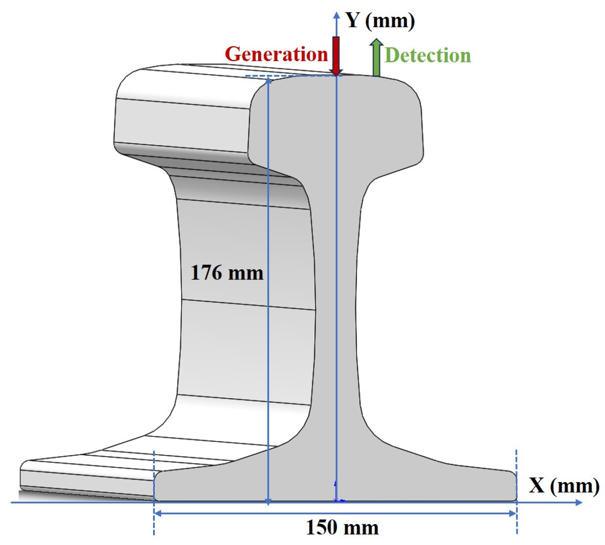
Using a 60 kg/m rail as a geometric model, the FEM established the physical process of laser-excited ultrasonic testing with rail surface cracks. Figure 1 presents the 3D model drawing of the rail, the parameters of the A60 rail material properties are shown in

Table 1. Physical properties of the A60 Rail.

Characteristic Parameters	A60 Rail
Density (kg/m3)	7840
Thermal expansion coefficient (K−1)	1.18 × 10−5
Heat capacity (J/(kg∙K))	475
Young modulus (Gpa)	210
Thermal conductivity (W/(m·K))	44.5
Poisson’s ratio	0.29

, and the incident pulsed laser parameters are shown in

Table 2. Parameters of pulsed laser.

Spot Radius (mm)	Monopulse-Energy (mJ)	Peak Power Density (W/m2)	Pulse Width (ns)
1	5	1.5915 × 1011	10

.

In numerical simulations, the time step affects the stability of the results. A more considerable time step results in less stable results. Too small a time step results in a long computation time. The spatial grid size affects the spatial sampling of wave modes. A too-large grid increases the numerical dispersion, while a too-small grid increases computation. Therefore, it is necessary to divide the grid and set the time step reasonably. The time step and grid settings are as follows:

$$∆t={\displaystyle \frac{1}{180f_{max}}}$$

(7)

$$∆x\le {\displaystyle \frac{C_R}{{20f}_{max}}}$$

(8)

where ∆t is the minimum time step, ∆x is the minimum grid size, and f_max is the maximum frequency of laser-excited ultrasound, expressed as

$$f_{max}={\displaystyle \frac{\sqrt{2}{C}_R}{\pi R_0}}$$

(9)

where C_R is the Rayleigh wave velocity of ultrasound propagating in the rail, calculated as follows:

$$C_R={\displaystyle \frac{0.87+1.12v}{1+v}}\sqrt{{\displaystyle \frac{E}{\rho }}}\sqrt{{\displaystyle \frac{1}{2\left(1+v\right)}}}$$

(10)

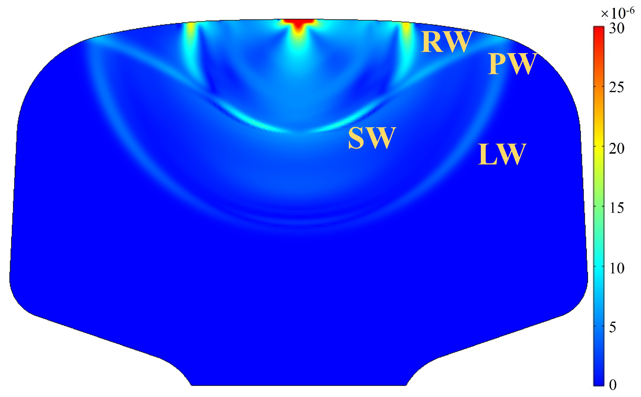
where v is Poisson’s ratio, E is Young’s modulus, and ρ is the material density, calculated as C_R = 2985 m/s. Since the rail is an isotropic material and symmetrical as a whole, the laser is uniformly distributed along the Z-axis direction, and the laser source tends to be infinitely long, the 3D model can be simplified to a 2D planar model for the study. To ensure that the simulation closely approximates the experiment, the outer boundary of the rail is set as a free boundary. Figure 2 presents the 2D acoustic field obtained from the simulation.

The result indicates that the shear wave (SW), the longitudinal wave (LW), the swept surface longitudinal wave (PW), and the Rayleigh wave (RW) are successfully excited. Among them, the amplitude of RW is significantly higher than that of the other waves and propagates along the rail head’s surface. Therefore, this paper uses RW to detect surface cracks.

3. Simulation Results and Analysis

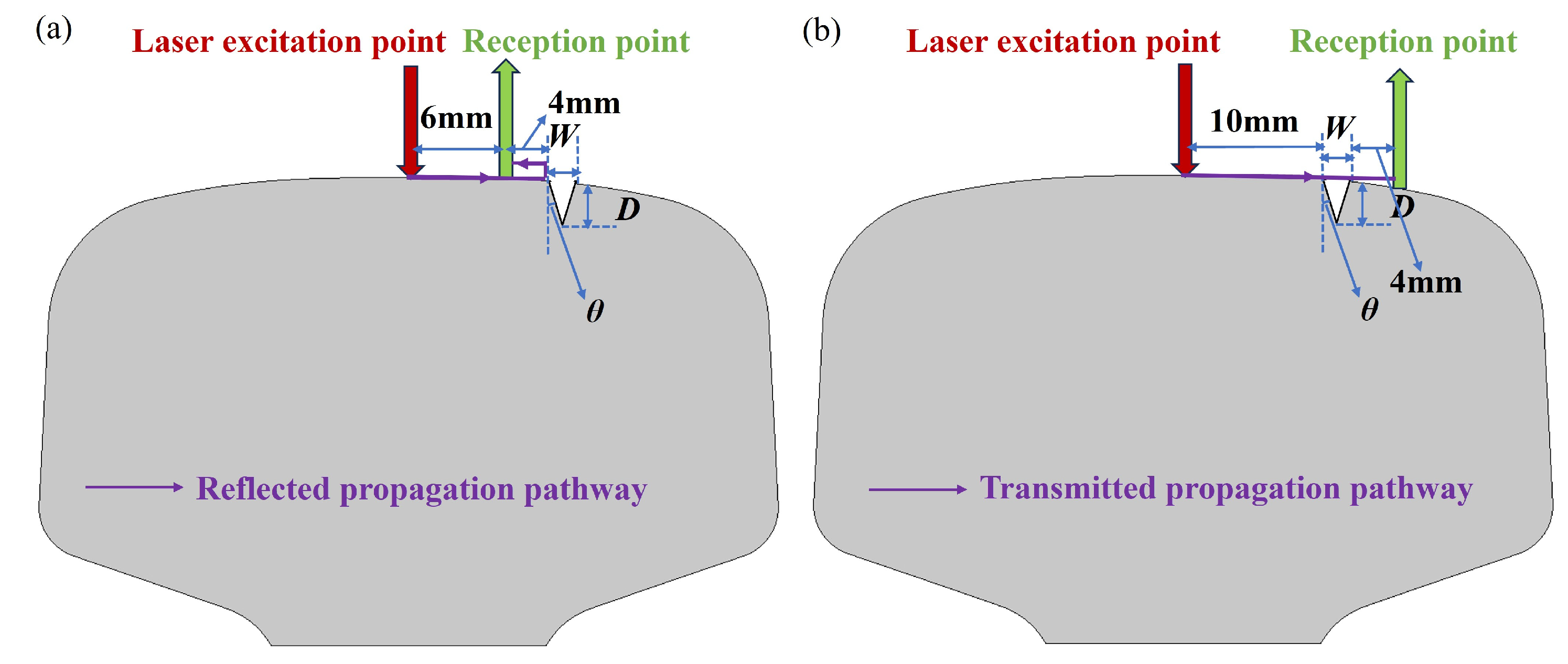
A comsol finite element simulation model was developed to study the process of laser ultrasound and surface cracks and to understand the propagation path of laser ultrasound in the rail specimen, as shown in Figure 3. The pulse-echo, pitch-catch, and TOF methods are the most representative methods for laser ultrasonic detection. Therefore, this paper uses these three methods to detect cracks and obtain the corresponding time-domain signals. The distance between the excitation and detection points is 6 mm for the pulse-echo method and 10 mm for the pitch-catch method. The vertical angle of the crack is θ, the depth is D, and the width is W.

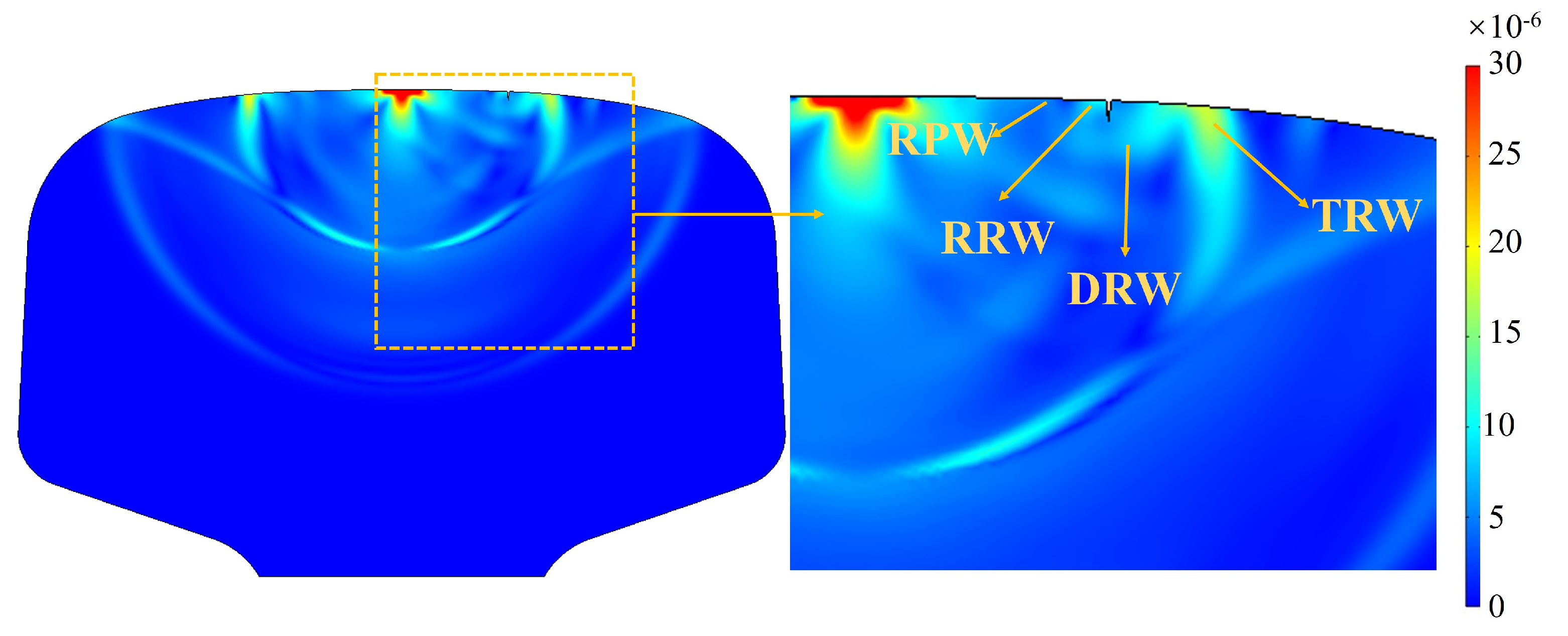
The pulse energy of the laser excitation is set to 5 mJ, the spot radius is 1 mm, and the pulse width is 10 ns, and the simulation results are obtained as shown in Figure 4. The PW wave is the fastest and encounters the defect first, and part of the sound wave is reflected by the defect, forming the RPW. The RW interacts with the crack, part of it is reflected by the crack to create a reflected Rayleigh wave (RRW), and part of it transmits through the crack to form a transmitted Rayleigh wave (TRW). In addition, a portion of the RW propagates along the crack to the crack tip and reaches the detection point as diffracted Rayleigh waves (DRW).

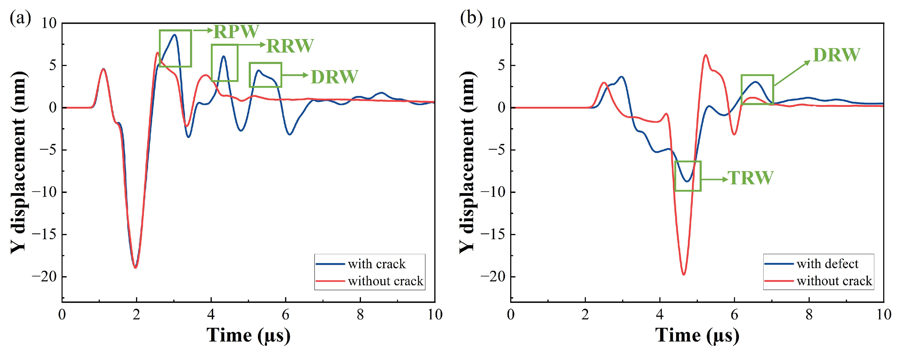
To determine which type of ultrasound can effectively characterize cracks, the stress displacements with and without cracks were compared, as shown in Figure 5. Figure 5a shows the stress displacement detected by the pulse-echo method, the width of the crack is 2 mm, the angle is 0°, and the depth is 2 mm. Figure 5b shows the stress displacement detected by the pitch-catch method, the width of the crack is 4 mm, the angle is 0°, and the depth is 6 mm. It can be seen that RPW, RRW, and DRW all contain information about cracks, and using these sound waves, cracks can be quantitatively detected. The propagation distance of the RW is 14 mm, and the theoretical RRW time is 4.69 µs. The figure shows that the RRW time is 4.40 µs, and the theoretical value is very close to the simulation result. It proves that the signal is the reflection echo signal and verifies the model’s accuracy.

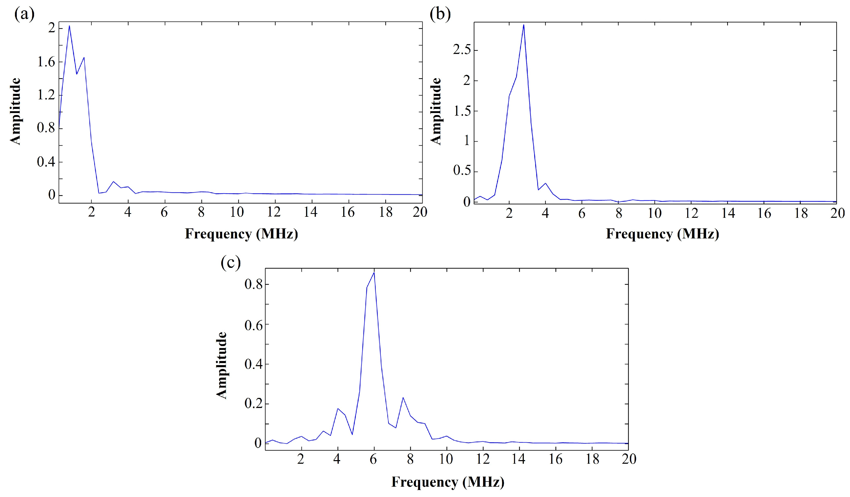
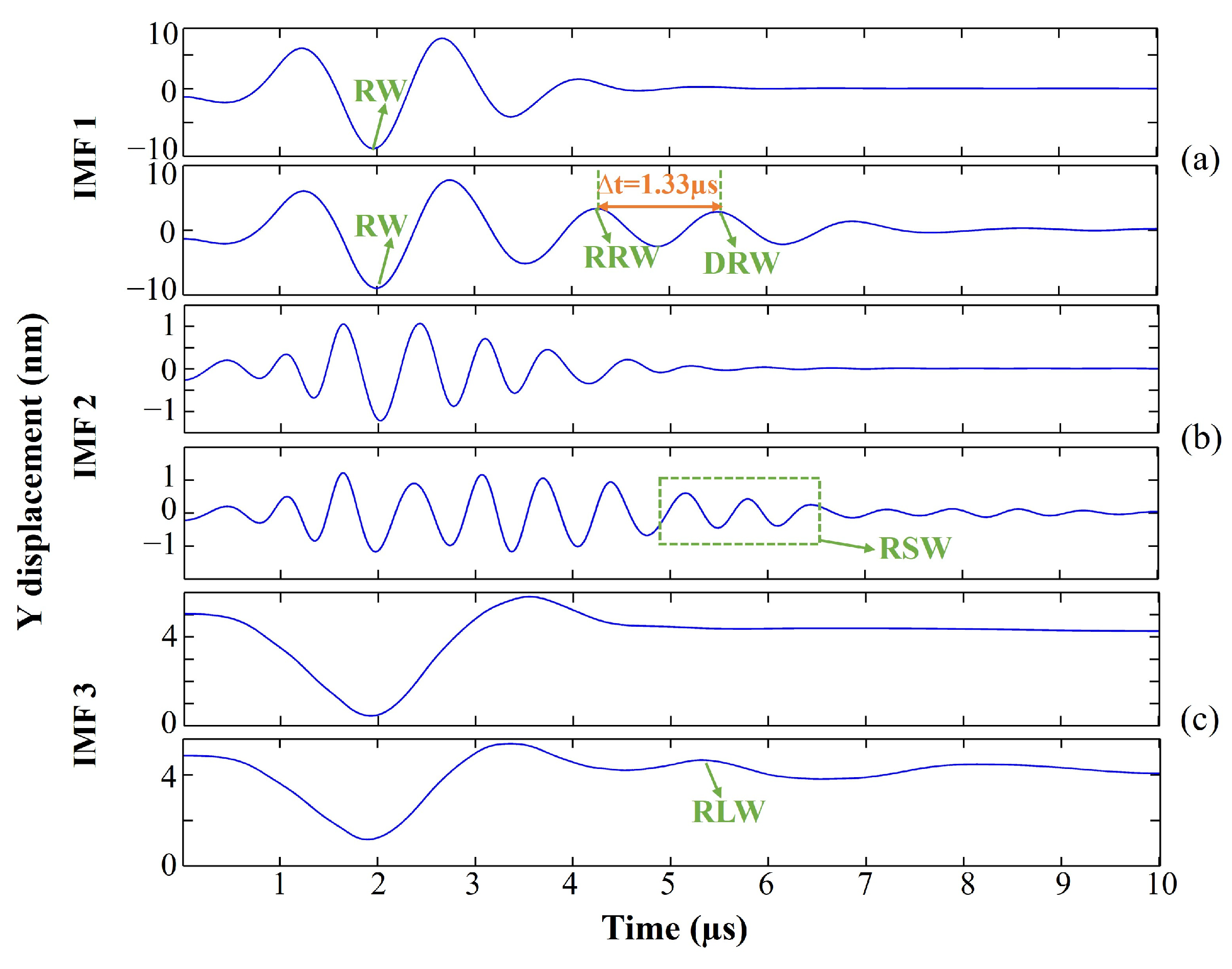
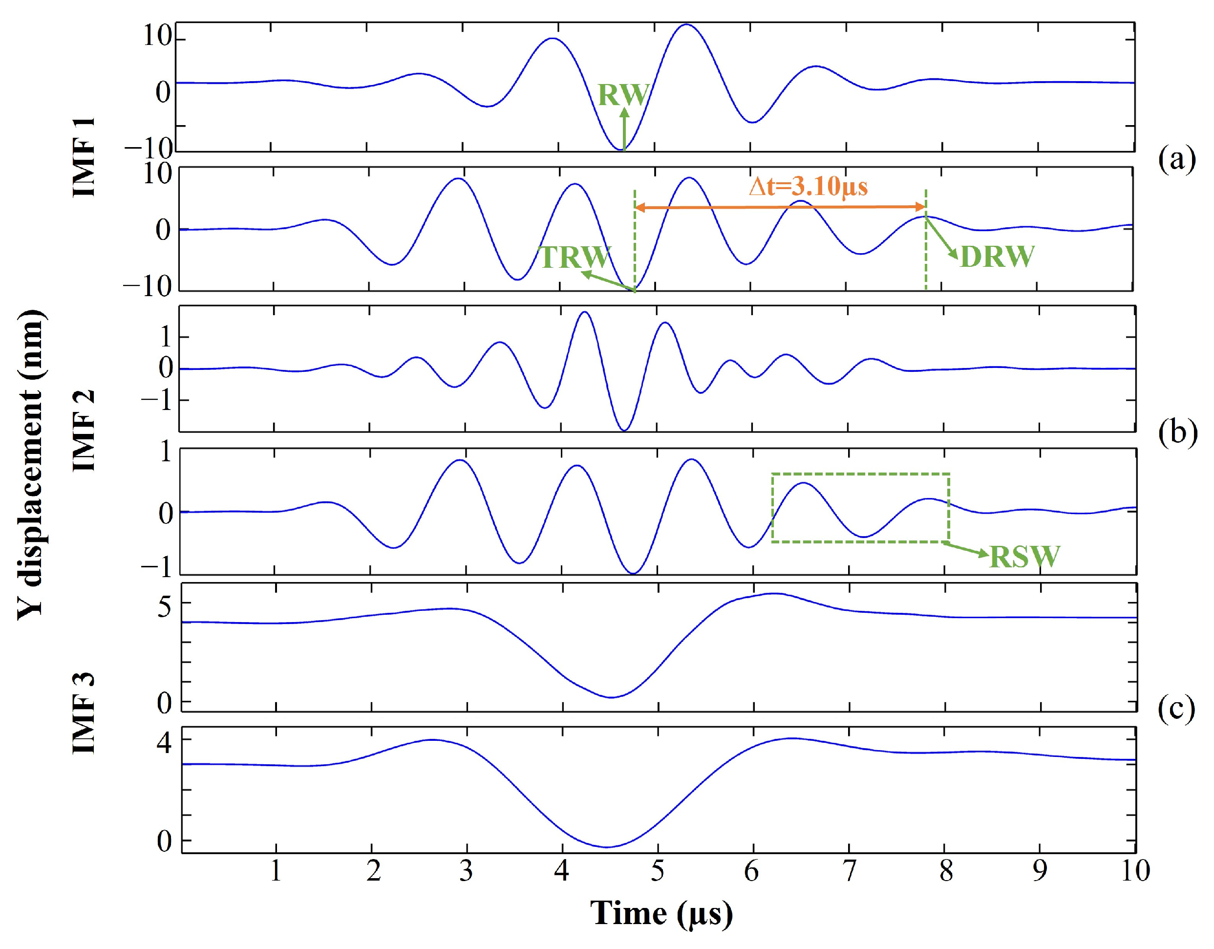
However, the composition of DRW is complex, and it is necessary to analyze it to characterize the cracks better using this waveform. Since broadband pulses excite different frequencies, using VMD can facilitate the identification of various wave packets. Therefore, decomposing simulated signals with VMD can clarify the types of ultrasonic waves present in the DRW. The frequency-domain signals obtained after VMD decomposition are shown in Figure 6. It can be observed that the center frequency increases with the addition of mode components. Based on the relationship between frequency and wave speed, it can be determined that IMF1 corresponds to the RW component, IMF2 to the shear wave component, and IMF3 to the longitudinal wave component. The time-domain diagram of the VMD decomposition obtained using the pulse-echo method is shown in Figure 7, while the diagram obtained using the pitch-catch method is presented in Figure 8. Comparing the modal decomposition plots with and without cracks reveals that the DRW includes both the RW propagating along the crack, the RW-converted shear wave (RSW), and the RW-converted longitudinal wave (RLW).

3.1. Determination of Crack Location

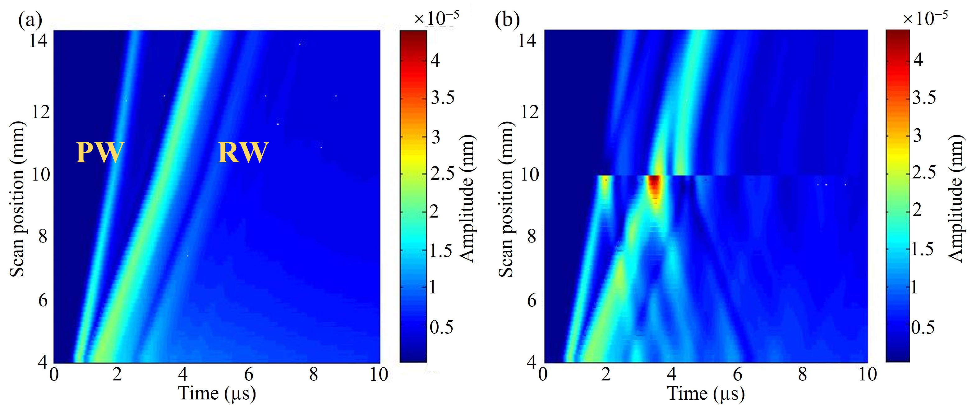
The position of the laser excitation point was fixed, and the receiving point was moved in steps of 0.01 mm so that its distance from the excitation point changed from 4 mm to 14 mm. Figure 9 shows that the acquired A-scan signal is plotted as a B-scan graph. Compared to the B-scan with no cracks, the B-scan with cracks has a clear waveform truncation at 10 mm from the excitation point. Therefore, the crack is located 10 mm from the excitation point, and the method can accurately determine the location of the crack.

3.2. Crack Angle Detection

When the crack depth is within 1.5 mm, regular grinding can maintain the rail. If the crack depth of the rail is over 1.5 mm, the crack may develop into a larger crack. Therefore, quantitatively identifying inclined cracks with a depth of 1.5 mm is essential for rapidly detecting rails.

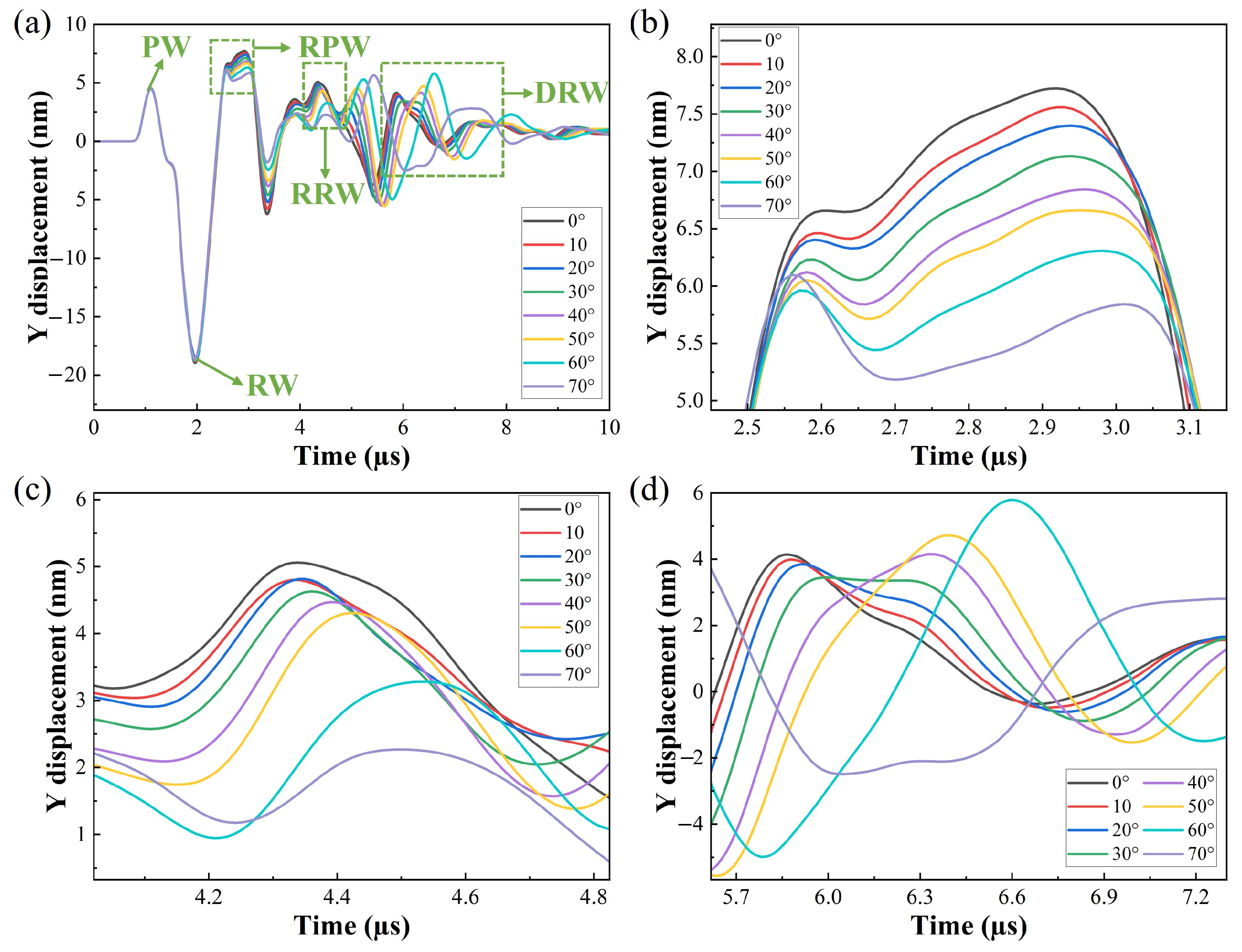
With fixed crack width of 0.2 mm, and depth of 1 mm, the crack’s vertical angle increased from 0° to 70°. The time-domain signal obtained based on the pulse-echo method is shown in Figure 10a, and the amplified RPW, RRW, and DRW sections are shown in Figure 10b–d. Theoretically, the peak displacement of RRW should be greater than DRW’s. However, after the crack angle is more significant than 40°, due to the continuous accumulation, DRW’s peak displacement is higher than the peak displacement of RRW.

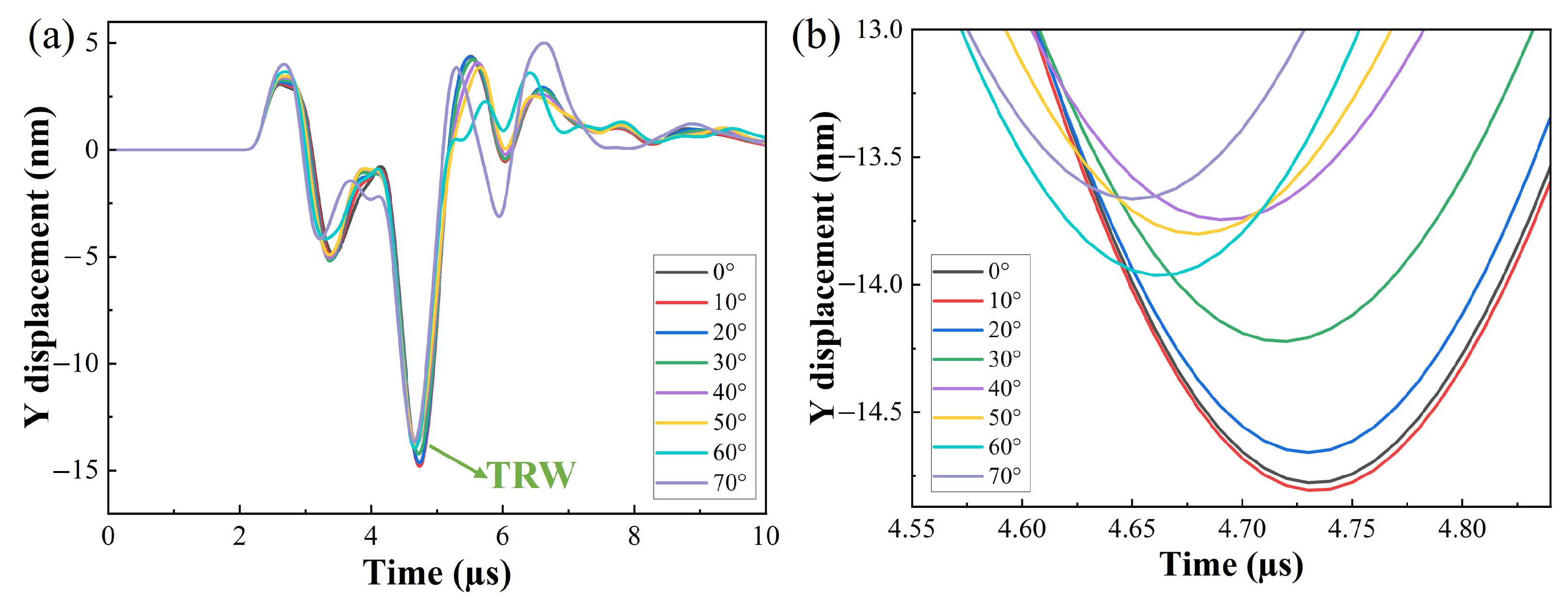
The time-domain signal obtained based on the pitch-catch method is shown in Figure 11a, and the magnified TRW part is shown in Figure 11b. It can be seen that the TRW changes irregularly for different angle cracks. Therefore, the pulse-echo method is more suitable to characterize the crack angle.

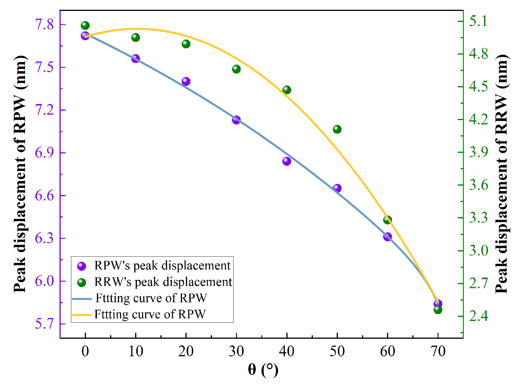
Based on the mentioned analysis, the useful signal carrying the crack information is fitted to the crack angle. Figure 12 shows the RPW and RRW peak stress displacements fitting with the angle obtained using the pulse-echo method. It can be seen that the RPW and RRW peak stress displacement is inversely proportional to the angle magnitude. This is because the more significant the angle, the more inclined the left edge of the crack and the weaker the ultrasound reflection effect. The regression coefficient R² of the RPW fitted curve is 99.806%, and the fitted curve equation is

$$Y=8.436-0.358exp\left({\displaystyle \frac{\theta }{48.915}}\right)-0.358 exp\left({\displaystyle \frac{\theta }{59.785}}\right)$$

(11)

The regression coefficient R² of the RRW fitted curve is 98.73%, and the fitted curve equation is

$$Y=4.956+0.014\theta -7.012\times {10}^{-4}{\theta }^2$$

(12)

In addition, the crack angle can be characterized using the TOF, as shown in Figure 13. The regression coefficient R² of the nonlinear curve fitting reaches 99.326%, and the expression of the fitted curve is

$$\Delta T=1.510+0.01exp\left({\displaystyle \frac{\theta }{14.347}}\right)$$

(13)

where ∆T is the time difference between RRW and DRW. The results show that the larger the vertical angle, the more significant the time difference. This is because, at a certain crack depth, the left edge of the crack increases with the angle. This causes the DRW propagation time to become longer, reaching the reception point with a corresponding delay. Therefore, the crack angle information can be obtained by measuring ∆T.

3.3. Crack Depth Detection

Fixing the crack at a vertical angle of 0° and a width of 0.2 mm increased the crack depth from 0.5 mm to 1.4 mm. Figure 14 presents the time-domain signal obtained using the pulse-echo method. As the crack depth is more significant, the reflection of ultrasonic waves by the crack is more substantial. Therefore, the stress displacement amplitude of RPW and RRW is proportional to the crack depth. While DRW propagates along the crack, its time increases with the crack depth.

Figure 15 presents the time-domain signal obtained using the pitch-catch method, where the smaller the crack depth is, the larger the amplitude of TRW is. This is because the more significant the depth, the less Rayleigh waves can be transmitted, so the stress displacement amplitude of the TRW is inversely proportional to the depth.

The valuable signal was fitted to the crack depth based on the analysis. Figure 16a shows the fitted curve of stress displacement amplitude with crack depth for RRW. The regression coefficient R² of the fitted curve reaches 99.827%, and the expression of the fitted curve is

$$Y=2.915+7.398D-2.322D^2$$

(14)

Figure 16b shows the fitting curve of the time difference between DRW and RRW with crack depth, R² = 98.628%, and the fitting equation is

$$∆T=2.23-{\displaystyle \frac{0.81}{1+exp\left[0.045\left(D-1.06\right)\right]}}$$

(15)

Figure 16c shows the fitted curve of stress displacement amplitude with crack depth for TRW. The regression coefficient of the fitted curve R² = 99.471%, and the expression of the fitted curve is

$$Y=0.59+0.037D+0.208D^2$$

(16)

Figure 16d shows the fitting curve of the time difference between DRW and TRW with crack depth, R² = 99.471%, and the fitting equation is

$$∆T=25.445-14.563D+2.17D^2$$

(17)

It can be seen that the DRW with RRW/TRW time difference increases with increasing crack depth. This is because, at a certain angle, the greater the depth, the longer the left edge of the crack. The time for the DRW to propagate along the left edge of the crack increases, and the time to reach the reception point is delayed accordingly.

3.4. Crack Width Detection

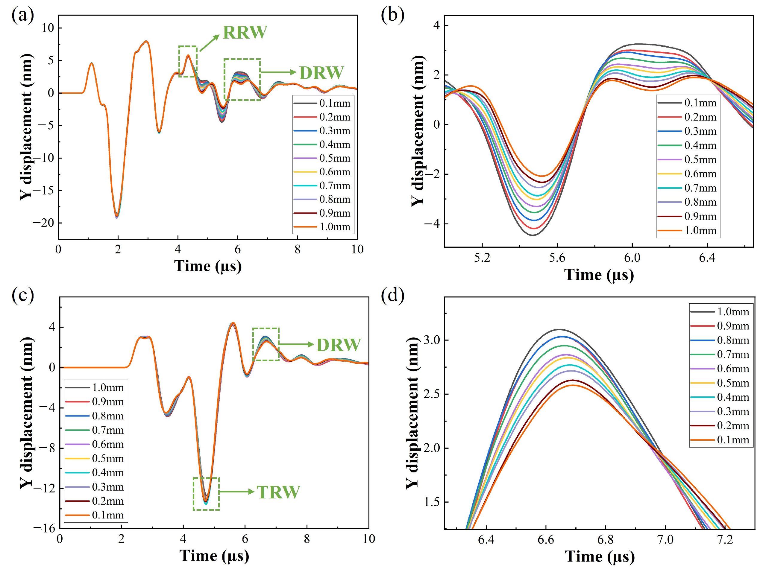
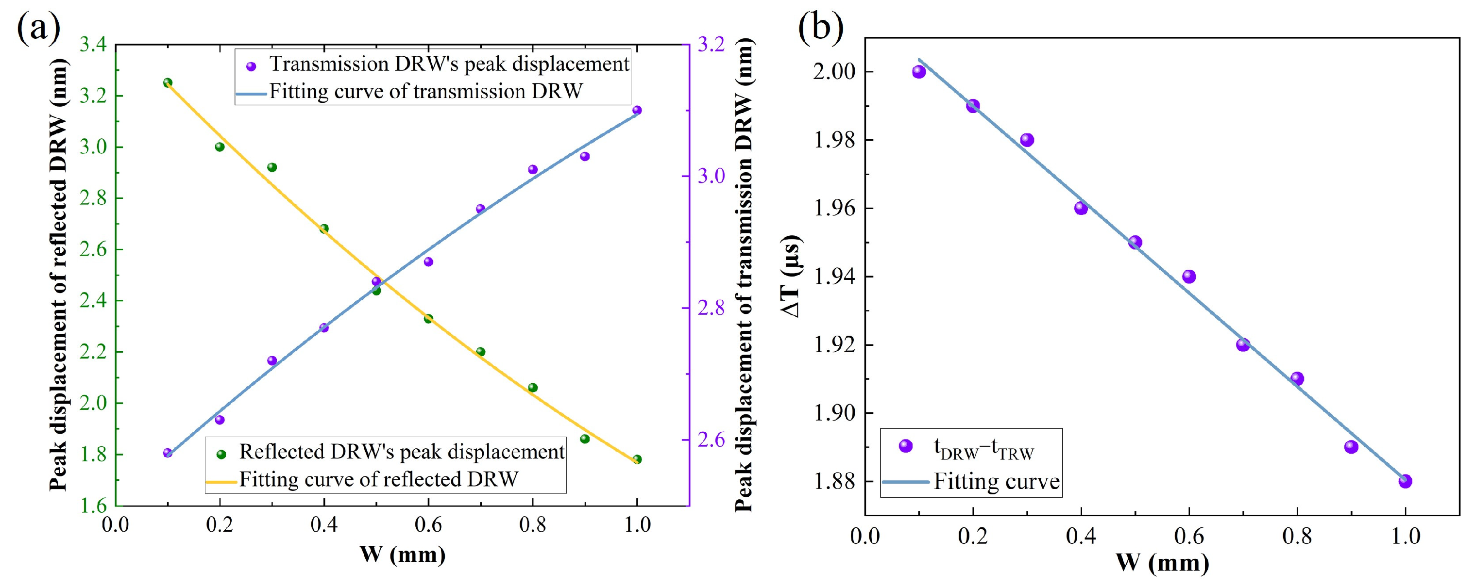
Fixing the crack at a vertical angle of 0° and a depth of 1.0 mm increased its width from 0.1 mm to 1.0 mm. Figure 17 shows the time-domain signals obtained using pulse-echo and pitch-catch methods. It can be seen that the width does not affect the time and amplitude of the RRW. However, as the width increases, the amplitude and time of the DRW stress displacement in the reflected and transmitted signals change regularly. Therefore, DRW is a helpful signal that can characterize the crack width. The stress displacement amplitude of DRW is fitted to the crack width to obtain the fitted curve in Figure 18a. The time difference between DRW and TRW is fitted to the crack width to obtain the fitted curve shown in Figure 18b. The R² of the reflected DRW is 99.374%, and the expression of the fitted curve is

$$Y=3.451-2.126W+0.447W^2$$

(18)

The R² of the transmission DRW is 99.532%, and the expression of the fitted curve is

$$Y=2.506+0.713W-0.125W^2$$

(19)

The R² of the fitted curve based on the TOF method is 99.374%, and the expression of the fitted curve is

$$\Delta T=2.017-0.137W$$

(20)

Based on the mentioned analysis, the maximum errors in crack size detection by different methods are summarized in

Table 3. Maximum error of crack detection by different methods.

	Pulse-Echo	Pitch-Catch	TOF
θ	9.44%	*	5.67%
D	0.84%	1.11%	1.67%
W	2.27%	1.72%	0.76%

In Table 3, * indicates that the method cannot characterize such cracks.

. The results show that the quantitative detection of rail surface cracks based on laser ultrasound is feasible, and the relative error of crack quantification is within 10%. Among them, the TOF method can detect arbitrary types of cracks with relatively small errors, which is an effective method for quantitatively detecting cracks.

4. Experimental Results

4.1. Experimental Setup and Samples

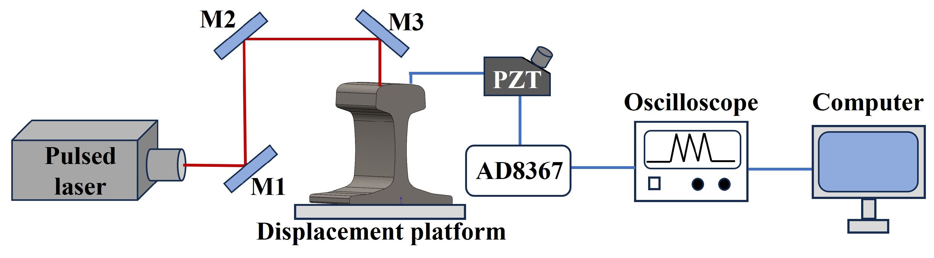
The LUT optical system for testing rail cracks is shown in Figure 19. A Nd: YAG pulsed laser constructed independently by the group was used as the ultrasonic excitation source. The laser beam is focused by the lens set to form a spot with a diameter of 1.0 mm. The sample is mounted on a displacement platform to control the relative position of the excitation–detection point, and the minimum movement distance of the displacement platform is 1.0 mm. Since this paper mainly uses surface acoustic waves to detect surface cracks, a surface wave piezoelectric probe is chosen to receive the ultrasonic signals generated by the laser. To better observe the detected ultrasonic signals, an AD8367 gain amplifier module was used to achieve linear gain amplification. The received signals were amplified by a preamplifier and recorded by an oscilloscope. The oscilloscope used is a Tektronix model, and the experimental results consist mainly of electrical signals displayed by the oscilloscope. The experimental parameters are shown in

Table 4. Experimental parameters.

Spot Radius	Pulse-Energy	Repetition Frequency	Pulse Width	AD8367-Maximum Gain	Sample Rate
1 mm	5 mJ	1 Hz	10 ns	45 dB	260 MSa/s

.

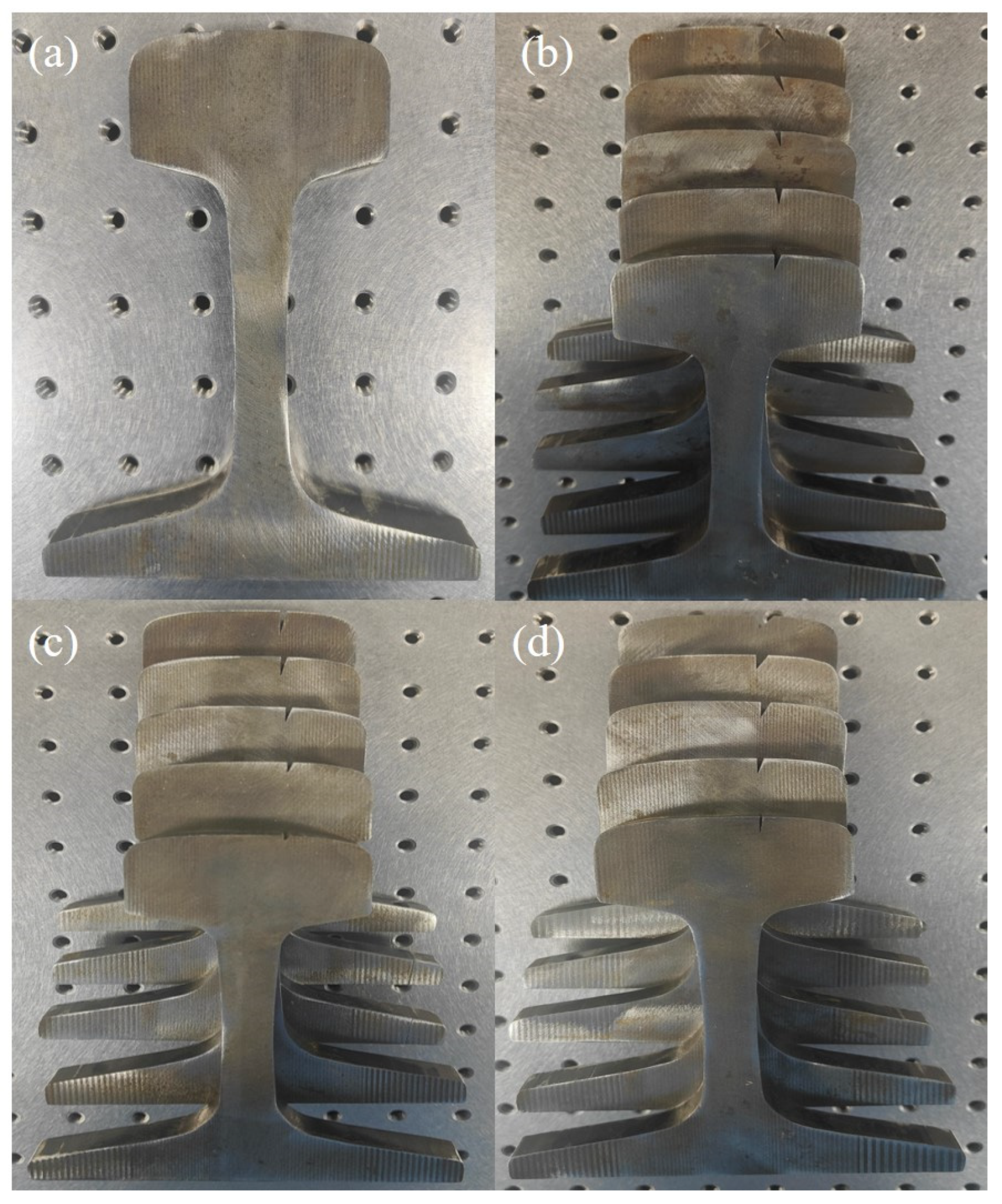
The sample was a 60 kg/m rail specimen cut into 15 mm thick sheets using wire cutting. On the rail head surface, cracks of different vertical angles, depths, and widths were cut, as shown in Figure 20. These rail specimens containing surface V-cracks with various parameters were used as test samples.

4.2. Crack Location Detection

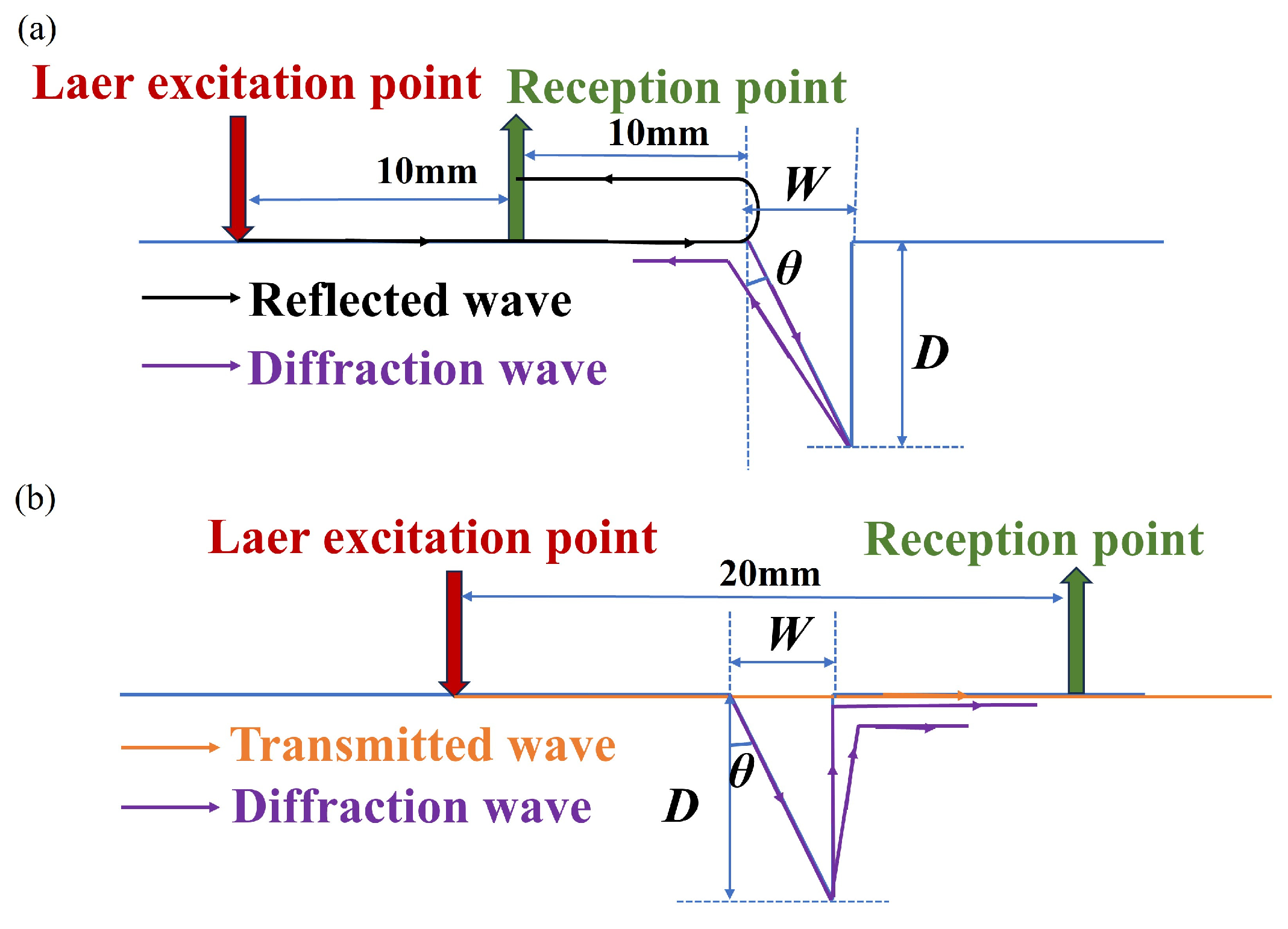
The fixed excitation–detection point distance is 10 mm, and the detection point is 10 mm away from the crack when the detection is based on the pulse-echo method, as shown in Figure 21a. The fixed excitation–detection point distance is 20 mm for the detection based on the pitch-catch method, as shown in Figure 21b.

Using the pulse-echo method shown in Figure 21a to detect the location of the crack, the crack location information can be derived from Equation (21).

$$x={\displaystyle \frac{∆t{C}_R}{2}}$$

(21)

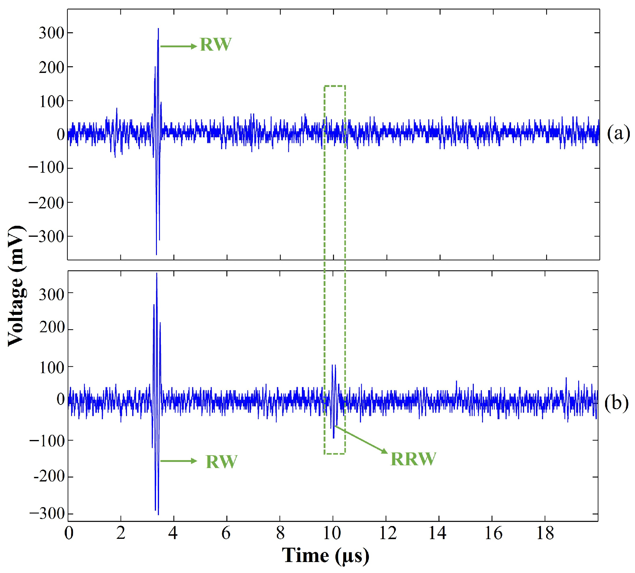
where x is the lateral distance from the defect to the detection point, ∆t is the time difference between RRW and RW, and C_R is the surface wave velocity. Figure 22 shows the ultrasonic signals obtained at the receiving point for the specimen with and without cracks. From the figure, it can be obtained that the time RW arrives at the detection point is 3.4 µs. According to the relationship between the RW speed and the propagation distance, the theoretical arrival time of the RW is 3.35 µs, with a relative error of 1.49%, which is a slight error. Compared with no crack, the ultrasonic signal with a crack has an obvious reflection echo signal RRW at 9.98 µs. According to the time of RRW arriving at the detection point, the distance of the crack from the detection point can be obtained from Equation (21), which is 9.85 mm, and the relative error is 1.5%. Therefore, the method can determine the location of the defect more accurately.

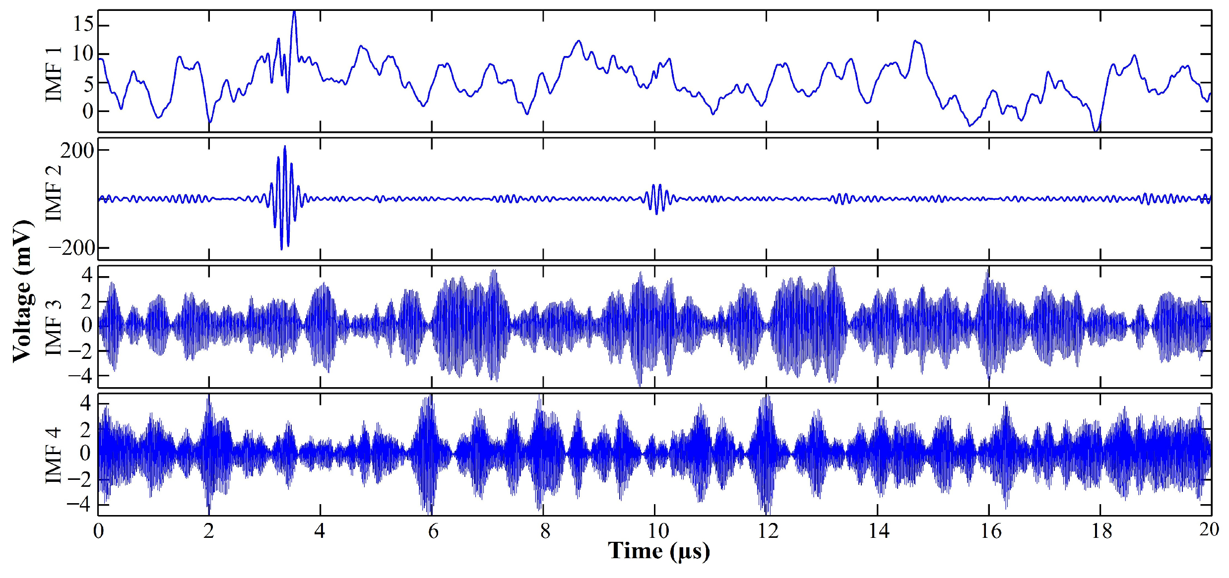
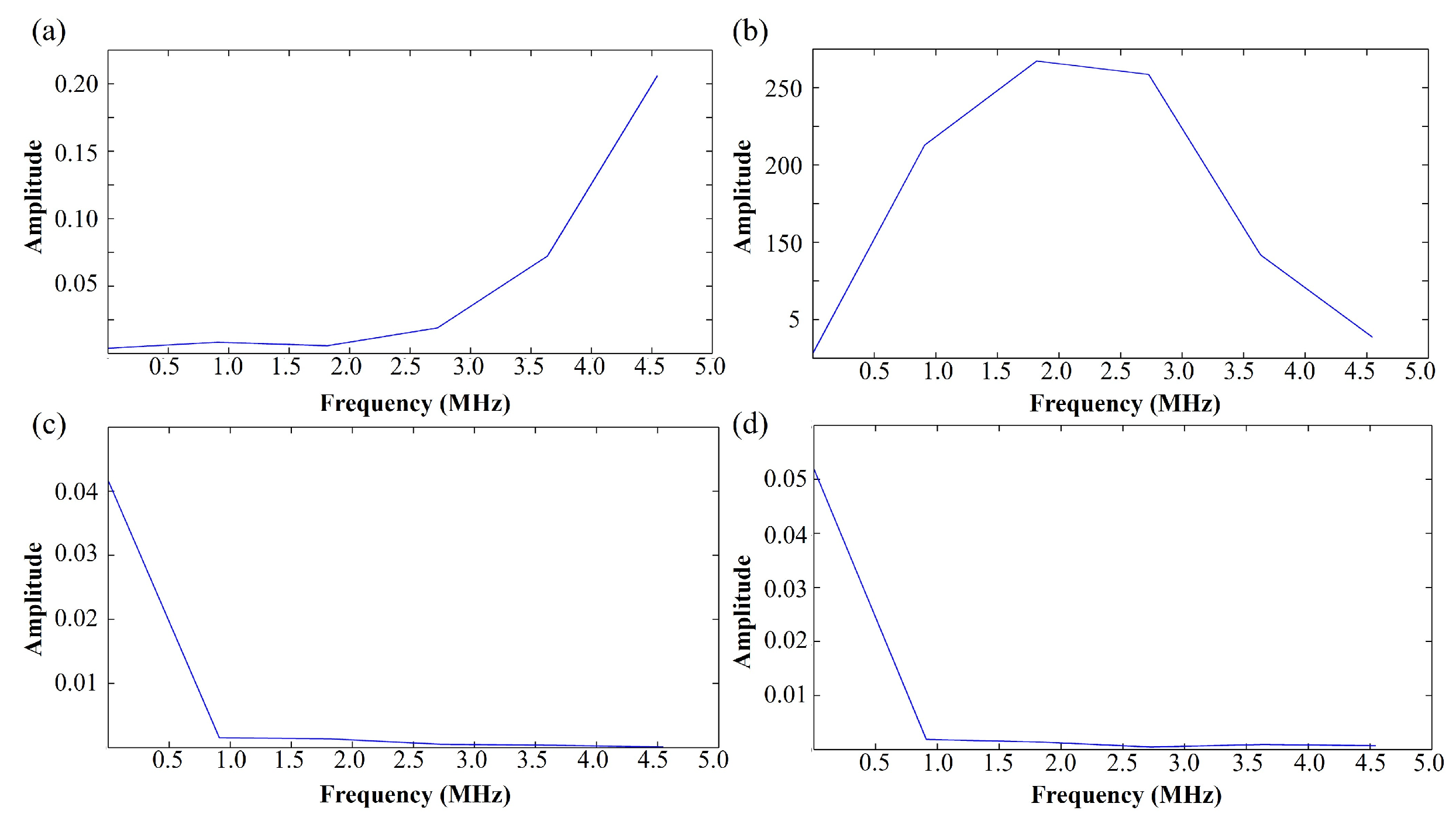
Reducing noise on the original signals is necessary to obtain ultrasound signals with a high signal-to-noise ratio. VMD allows each mode to reveal different signal characteristics by decomposing a complex signal into several eigenmodes. This decomposition helps to increase the detection sensitivity of minor defects, enhances the signal’s clarity, and helps extract useful detection information from the noise, thus improving the overall detection accuracy and reliability. This paper applies the VMD algorithm to the modal separation study of laser ultrasonic signals to obtain the clearest surface wave modes that characterize the crack information. The core of VMD is the signal decomposition into a series of intrinsic modes (IMFs) through a variational optimization model. Each mode has a different center frequency and bandwidth. The key to the VMD decomposition of the signal is to determine the number of modal components K. Based on the experience, K is set to 4 to satisfy the principle of no under-decomposition and no over-decomposition, which effectively improves the signal-to-noise ratio while obtaining the best characterization of different wave modes. The time–frequency-domain decomposition of the ultrasound signal shown in Figure 22b is performed, and the decomposed time-domain signal is shown in Figure 23. The frequency-domain signal is shown in Figure 24. It can be seen that IMF1 is separated as a high-frequency noise, and both IMF3 and IMF4 are separated as low-frequency noise. The center frequency of IMF2 is 2.5–3.0 MHz, and the energy is mainly concentrated in the range of 0–3 MHz, consistent with surface wave frequency. Moreover, the RW and RRW in this mode are visible, making it an effective mode for detecting crack information. Therefore, the decomposed IMF2 mode is used for all subsequent tests.

4.3. Crack Angle Detection

The distance between the detection and excitation points is fixed at 20 mm, and the detection point is 5 mm to the left of the crack. The amplitude of ultrasound is strongly influenced by the pulse energy and the experimental environment, while the pulse energy has small fluctuations. Therefore, using the ultrasonic signal’s amplitude to characterize the defect’s size will have a significant error. The TOF method can overcome the effect of pulse energy on the ultrasonic waves. Therefore, the ultrasonic signals obtained from the experiments were analyzed using the TOF method to characterize the defect size. The above simulation results show that the DRW contains much information about the defects. By calculating the time difference ∆t between RRW and DRW, the size of the defect can be quantitatively detected.

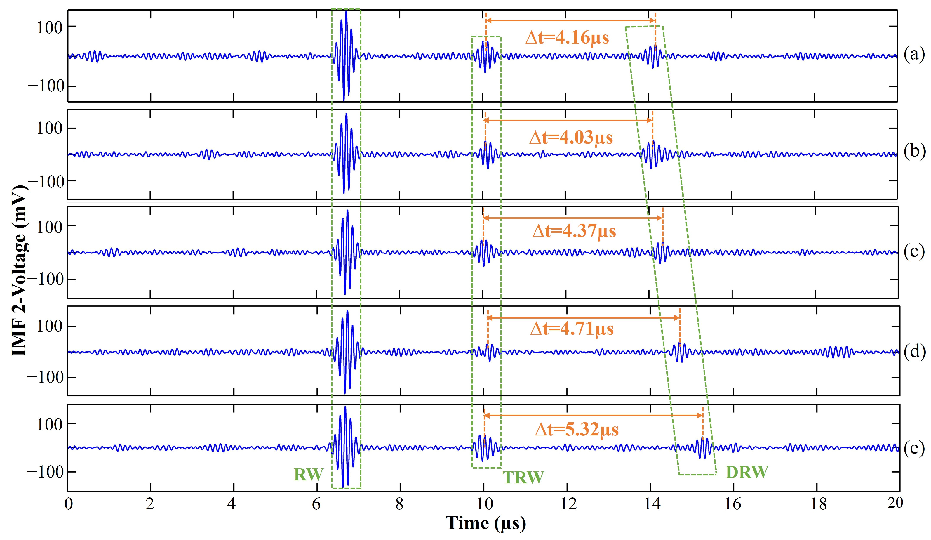
To investigate the effect of crack angle on the ultrasonic signal, the depth of the crack was fixed at 6 mm, and the width at 2 mm, and the vertical angle of the crack was varied to 0°, 10°, 20°, 30°, and 40°, as shown in Figure 20b. The ultrasonic signal waveform is shown in Figure 25.

Theoretically, the relationship between θ and ∆t is as follows:

$$\mathrm{c}\mathrm{o}\mathrm{s}\theta ={\displaystyle \frac{2D}{∆t{C}_R}}$$

(22)

where θ is the vertical angle of the crack, ∆t is the time difference between RRW and RW, and D is the depth of the crack. From the figure, it can be obtained that ∆t is 4.16 µs, 4.03 µs, 4.37 µs, 4.71 µs, and 5.32 µs; cosθ calculated from Equation (22) is 0.97, 1.00, 0.92, 0.85, and 0.76, with relative errors of 3.00%, 2.04%, 2.13%, 2.30%, and 1.30%, respectively. The relative errors are all within 3%, and the method is more accurate for detecting the vertical angle of cracks.

4.4. Crack Depth Detection

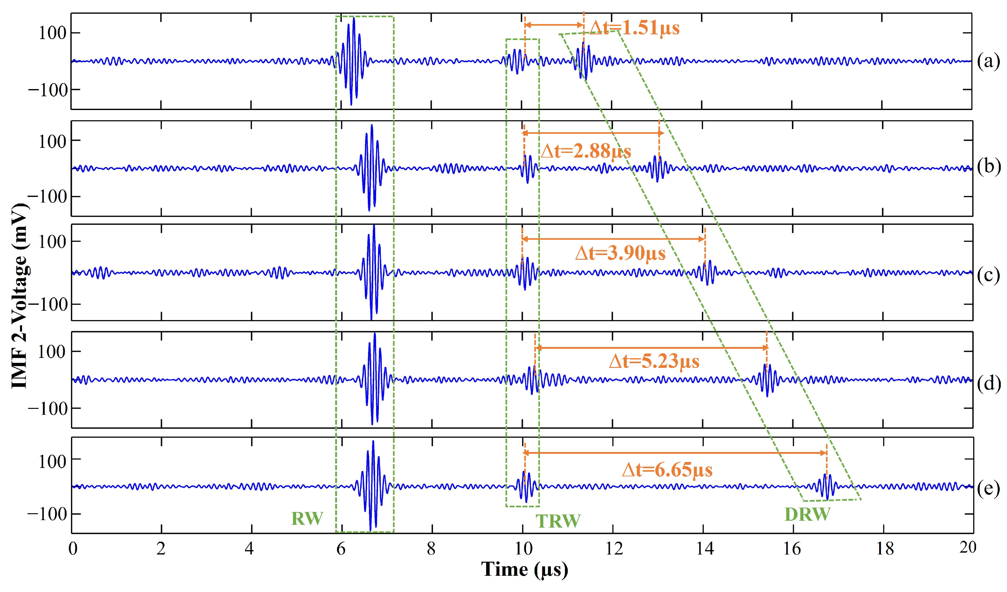
To investigate the effect of crack depth on the ultrasonic signal, the angle of the crack was fixed at 0°, the width was 2 mm, and the depth of the crack was varied to be 2 mm, 4 mm, 6 mm, 8 mm, and 10 mm, as shown in Figure 20c. The ultrasonic signal waveform is shown in Figure 26.

Theoretically, the relationship between D and ∆t is as follows:

$$D={\displaystyle \frac{∆t{C}_R\mathrm{c}\mathrm{o}\mathrm{s}\theta }{2}}$$

(23)

where ∆t is the time difference between RRW and DRW; from the figure, ∆t can be obtained as 1.51 µs, 2.88 µs, 3.90 µs, 5.23 µs, and 6.65 µs. The D calculated according to Equation (23) is 2.25 mm, 4.30 mm, 5.82 mm, 7.81 mm, and 9.93 mm, with a relative error of 12.50%, 7.50%, 3.00%, 2.38%, and 0.70%, respectively. It can be seen that for small-size cracks (D ≤ 4 mm), the detection error is more significant. This is because cracks with smaller depths are less reflective of RW, which leads to a more significant difference between the time of RW and the theoretical calculation. Therefore, further research is needed for small defect crack detection.

4.5. Crack Width Detection

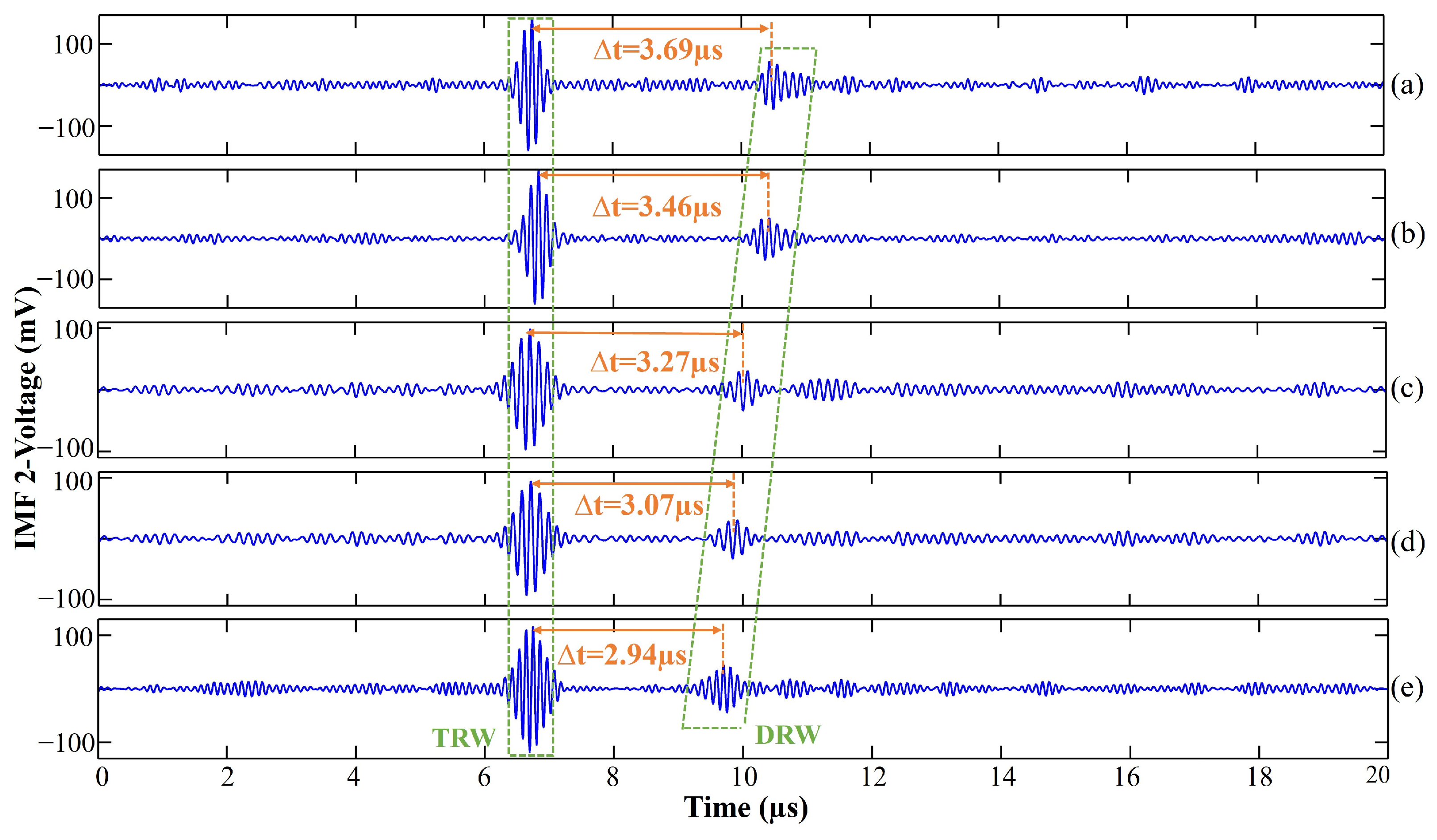
To investigate the effect of crack width on the ultrasonic signal, the angle of the crack was fixed at 0°, the depth was 6 mm, and the width of the crack was varied to 1 mm, 2 mm, 3 mm, 4 mm, and 5 mm, as shown in Figure 20d. From the simulation results, it is clear that the pulse-echo method is not suitable for detecting the crack width. Therefore, the pitch-catch method is used to detect the crack width. The distance between the excitation–detection point is 20 mm, the excitation point is located on the left side of the crack, and the detection point is located on the right side of the crack. The ultrasonic signal waveform is shown in Figure 27.

Theoretically, the relationship between W and ∆t is as follows:

$$∆t={\displaystyle \frac{L\mathrm{c}\mathrm{o}\mathrm{s}\theta -W\mathrm{c}\mathrm{o}\mathrm{s}\theta +D}{C_R\mathrm{c}\mathrm{o}\mathrm{s}\theta }}$$

(24)

$$W=\sqrt{L^2-D^2}$$

(25)

where ∆t is the time difference between DRW and TRW, and L is the length of the right edge of the crack. From the figure, ∆t is 3.69 µs, 3.46 µs, 3.27 µs, 3.07 µs, and 2.94 µs, respectively. The W is calculated according to Eqs. 24 and 25 are 1.03 mm, 1.99 mm, 2.91 mm, 4.12 mm, and 5.08 mm, with a relative error of 3.00%, 0.50%, 3.00%, 3.00%, 3.00%, and 1.70%, respectively. The results show that the method can effectively detect the crack width information.

Figure 26a shows that the time difference between DRW and RRW is 1.51 µs when the angle is 0°, width is 2 mm, and depth is 2 mm. In the simulation, the results for detecting the same size crack are presented in Figure 7a, where the time difference between DRW and RRW is 1.34 µs. From Figure 27d, the time difference between DRW and RRW is 3.07 µs when the angle is 0°, width is 4 mm, and depth is 6 mm, while in the simulation, the detection result for the same size crack is shown in Figure 8a with a time difference of 3.10 µs. It can be seen that the simulation results are consistent with the experimental results when only RW is present. The TOF method based on the DRW is an effective method for detecting crack information.

5. Discussions

Most reported rail defect detection studies focus on the qualitative detection of defects, which is insufficient. Quantitative testing can assess the severity of defects and identify potential defects to prevent railroad accidents caused by track problems. This paper presents a simple and effective method for quantitative detection of rail defects through simulation-guided experiments. In the simulation study, the interaction of various modes of ultrasound with cracks was analyzed. The results show that arbitrary types of cracks can be characterized using the TOF of DRW. This is because the DRW propagates along the crack and can be detected either by the pulse-echo method or by the pitch-catch method. The detection errors of this method are 1.83%, 1.67%, and 0.76% for angle, depth, and width, which are small errors. While DRW is an effective waveform for characterizing crack size, the simulation results indicate that the DRW components are complex. To explore the composition of DRW, the simulated signal is decomposed using VMD. The analysis shows that the DRW comprises the RW propagating along the crack, the RSW, and the RLW. Since DRW is not easily separated from other waveforms, the identification of DRW will be more difficult in experimental environments where noise is present. To solve this problem, the experiment uses a contact surface wave transducer to receive ultrasound signals. The received DRW are all surface waves, which can be clearly separated from RRW and TRW. Although contact transducers usually have low background noise, there is still experimental noise. The VMD technique is used to process the ultrasonic signal, separating the modal components from the noise. Based on the corresponding frequencies of each mode, IMF2 mainly exhibits surface wave characteristics, making it an effective mode for detecting surface cracks. Future research will focus on further optimizing the VMD algorithm for its application in detecting internal rail defects.

6. Conclusions

This paper combines the FEM of laser-excited ultrasound with experiments to detect V-cracks on the rail surface quantitatively. The interaction process between ultrasonic waves and cracks was analyzed in a finite element simulation model, and the amplitude and time of the relevant ultrasonic signals were selected and fitted to the crack size. The relationship between the ultrasonic signal and the crack size can be obtained visually through the fitting formula, which achieves quantitative detection. In the experiments, to solve the problem of low signal-to-noise ratio of ultrasound signals, a method of extracting the eigenmodes of clearly visible ultrasound using VMD is proposed. Since the energy will not be constant all the time in the experimental environment, the method of using the amplitude of the ultrasonic signal to characterize the crack size in FEM is not reliable. The time for the ultrasonic signal to reach the detection point is only related to its propagation speed and distance traveled. Therefore, the TOF method was used in the experiments to detect the crack size. The results show that the method can effectively detect the crack size. The relative error of localization is 1.39%, and the relative error of quantification is mostly within 8%.

References

- Zhao, X.; Wang, H.; Guo, J.; Liu, Q.; Zhao, G.; Wang, W. The effect of decarburized layer on rolling contact fatigue of rail materials under dry-wet conditions. Eng. Fail. Anal. 2018, 91, 58–71. [Google Scholar] [CrossRef]
- Steenbergen, M. Rolling contact fatigue: Spalling versus transverse fracture of rails. Wear 2017, 380–381, 96–105. [Google Scholar] [CrossRef]
- Zhang, Y.; Dang, D.; Wang, Y.; Ni, Y. Damage identification for railway tracks using ultrasound guided wave and hybrid probabilistic deep learning. Constr. Build. Mater. 2024, 418, 135466. [Google Scholar] [CrossRef]
- Xu, P.; Chen, Y.; Liu, L.; Liu, B. Study on high-speed rail defect detection methods based on ECT, MFL testing and ACFM. Measurement 2023, 206, 112213. [Google Scholar] [CrossRef]
- Liu, Z.; Li, W.; Xue, F.; Xia, F.; Jun, Y.; Bu, B.; Yi, Z. Electromagnetic Tomography Rail Defect Inspection. IEEE Trans. Magn. 2015, 51, 6201907. [Google Scholar] [CrossRef]
- Li, Y.; Tian, G.; Ward, S. Numerical simulation on magnetic flux leakage evaluation at high speed. NDT E Int. 2005, 39, 367–373. [Google Scholar] [CrossRef]
- Ohara, Y.; Nakajima, H.; Tsuji, T.; Mihara, T. Nonlinear surface-acoustic-wave phased array with fixed-voltage fundamental wave amplitude difference for imaging closed cracks. NDT E Int. 2019, 108, 102170. [Google Scholar] [CrossRef]
- Okuyama, N.; Nomura, K.; Sano, T.; Kadota, K.; Nitta, S.; Era, T.; Asai, S. Study on Detecting Method of Internal Defects by Laser Ultrasonics in Lap Joint Welding of Galvanized Steel Sheet and Finite Element Analysis of Its Detectability. Appl. Sci. 2023, 13, 11515. [Google Scholar] [CrossRef]
- Anandika, R.; Lundberg, J.; Stenström, C. Phased array ultrasonic inspection of near-surface cracks in a railhead and its verification with rail slicing. Insight 2020, 62, 387–395. [Google Scholar] [CrossRef]
- Kim, G.; Seo, M.-K.; Kim, Y.-I.; Kwon, S.; Kim, K.-B. Development of phased array ultrasonic system for detecting rail cracks. Sens. Actuators A Phys. 2020, 311, 112086. [Google Scholar] [CrossRef]
- Gao, F.; Zhou, H.; Huang, C. Defect detection using the phased-array laser ultrasonic crack diffraction enhancement method. Opt. Commun. 2020, 474, 126070. [Google Scholar] [CrossRef]
- Lian, Y.; Du, F.; Xie, L.; Hu, Q.; Jin, P.; Wang, Y.; Lu, Z. Application of laser ultrasonic testing technology in the characterization of material Properties: A review. Measurement 2024, 234, 114855. [Google Scholar] [CrossRef]
- Xie, L.; Lian, Y.; Du, F.; Wang, Y.; Lu, Z. Optical methods of laser ultrasonic testing technology in the industrial and engineering applications: A review. Opt. Laser Technol. 2024, 176, 110876. [Google Scholar] [CrossRef]
- Pathak, M.; Alahakoon, S.; Spiryagin, M.; Cole, C. Rail foot flaw detection based on a laser induced ultrasonic guided wave method. Measurement 2019, 148, 106922. [Google Scholar] [CrossRef]
- Allam, A.; Alfahmi, O.; Patel, H.; Sugino, C.; Harding, M.; Ruzzene, M.; Erturk, A. Ultrasonic testing of thick and thin Inconel 625 alloys manufactured by laser powder bed fusion. Ultrasonics 2022, 125, 106780. [Google Scholar] [CrossRef]
- Zhao, Y.; Jia, Z.Q.; Rui, G.; Ma, J.; Song, J.F.; Sun, J.H.; Liu, S. The Application of Laser-EMAT Technique Used to Testing Defect in Rail. Adv. Mater. Res. 2014, 875–877, 574–577. [Google Scholar] [CrossRef]
- Liu, Y.; Yang, S.; Liu, X. Detection and Quantification of Damage in Metallic Structures by Laser-Generated Ultrasonics. Appl. Sci. 2018, 8, 8050824. [Google Scholar] [CrossRef]
- Huang, Q.; Xie, L.; Yin, G.; Ran, M.; Liu, X.; Zheng, J. Acoustic signal analysis for detecting defects inside an arc magnet using a combination of variational mode decomposition and beetle antennae search. ISA Trans. 2020, 102, 347–364. [Google Scholar] [CrossRef]
- Sun, Y.; Ni, C.; Ying, K.; Xiong, A.; Shuai, T.; Shen, Z. Laser ultrasonic spatially resolved acoustic spectroscopy for grain size study based on Improved Variational Mode Decomposition (IVMD). NDT E Int. 2024, 144, 103090. [Google Scholar] [CrossRef]
- Gschwandl, T.J.; Weniger, T.M.; Antretter, T.; Künstner, D.; Scheriau, S.; Daves, W. Experimental and Numerical Visualisation of Subsurface Rail Deformation in a Full-Scale Wheel–Rail Test Rig. Metals 2023, 13, 1089. [Google Scholar] [CrossRef]
- Zhu, L.; Duan, X.; Yu, Z. On the Identification of Elastic Moduli of In-Service Rail by Ultrasonic Guided Waves. Sensors 2020, 20, 1769. [Google Scholar] [CrossRef] [PubMed]
- Wang, Y.; Han, S.; Yu, Y.; Qi, X.; Zhang, Y.; Lian, Y.; Bai, Z.; Wang, Y.; Lv, Z. Numerical Simulation of Metal Defect Detection Based on Laser Ultrasound. IEEE Photonics J. 2021, 13, 1–9. [Google Scholar] [CrossRef]
- Han, S.; Lian, Y.; Xie, L.; Hu, Q.; Ding, J.; Wang, Y.; Lu, Z. Numerical simulation of angled surface crack detection based on laser ultrasound. Front. Phys. 2022, 10, 982232. [Google Scholar] [CrossRef]
- Xu, Z.; Tian, Q.; Hu, P.; Li, H.; Shen, S. Laser ultrasonic detection of submillimeter artificial holes in laser powder bed fusion manufactured alloys. Opt. Laser Technol. 2024, 169, 110030. [Google Scholar] [CrossRef]
Disclaimer/Publisher’s Note: The statements, opinions and data contained in all publications are solely those of the individual author(s) and contributor(s) and not of MDPI and/or the editor(s). MDPI and/or the editor(s) disclaim responsibility for any injury to people or property resulting from any ideas, methods, instructions or products referred to in the content. |
© 2024 by the authors. Licensee MDPI, Basel, Switzerland. This article is an open access article distributed under the terms and conditions of the Creative Commons Attribution (CC BY) license (https://creativecommons.org/licenses/by/4.0/).