Abstract
In September 2018, NASA launched the ICESat-2 satellite into a 500 km high Earth orbit. It carried a truly unique lidar system, i.e., the Advanced Topographic Laser Altimeter System or ATLAS. The ATLAS lidar is capable of detecting single photons reflected from a wide variety of terrain (land, ice, tree leaves, and underlying terrain) and even performing bathymetric measurements due to its green wavelength. The system uses a single 5-watt, Q-switched laser producing a 10 kHz train of sub-nanosecond pulses, each containing 500 microjoules of energy. The beam is then split into three “strong” and three “weak” beamlets, with the “strong” beamlets containing four times the power of the “weak” beamlets in order to satisfy a wide range of Earth science goals. Thus, ATLAS is capable of making up to 60,000 surface measurements per second compared to the 40 measurements per second made by its predecessor multiphoton instrument, the Geoscience Laser Altimeter System (GLAS) on ICESat-1, which was terminated after several years of operation in 2009. Low deadtime timing electronics are combined with highly effective noise filtering algorithms to extract the spatially correlated surface photons from the solar and/or electronic background noise. The present paper describes how the ATLAS system evolved from a series of unique and seemingly unconnected personal experiences of the author in the fields of satellite laser ranging, optical antennas and space communications, Q-switched laser theory, and airborne single photon lidars.
1. Introduction
Theodore Maiman at the Hughes Research Laboratory in California reported the first ruby laser in 1960 [1], and the National Aeronautics and Space Administration (NASA) in the USA was quick to identify and implement potential space applications. In 1964, Dr. Henry H. Plotkin, Head of the Instrument Electro-optics Branch at the NASA Goddard Space Flight Center (GSFC), led a team that, on 31 October 1964, measured the distance to a satellite, Explorer 22B, by transmitting Q-switched ruby laser pulses at 1 Hz to a collection of retroreflectors mounted on the satellite, which reflected the pulse back to the ground station [2]. The telescope, located at the Goddard Optical Research Facility (GORF) a few miles from GSFC, was guided by two individuals seated on the telescope and independently controlling the azimuth and elevation axes to keep the telescope crosshairs on the sunlit satellite at night. By measuring the roundtrip time of flight (TOF) and multiplying by the speed of light, one could then compute the distance to the satellite for precise orbit determination. At the time, I was a first-year cooperative work/study student at GSFC and was honored to serve as a junior member of Dr. Plotkin’s SLR team following my freshman year at Drexel Institute of Technology (now Drexel University) in Philadelphia. Upon graduating from Drexel with a B.S. in Physics in 1968, I was offered a permanent position in Dr. Plotkin’s branch. Daylight ranging using computer-driven telescopes was first achieved by GSFC’s Don Premo in 1969. The earliest Satellite Laser Ranging (SLR) measurements were accurate to about 2 m, representing roughly a factor of 40 improvement relative to earlier radar measurements. The accuracy was limited by a number of factors, including the temporal width of the Q-switched ruby laser pulse (~1 µs), variable propagation times within the early photomultiplier tube detectors which amplified the weak return signals, the precision of the electronics measuring the time interval between the start and stop event, the temporal broadening of the return pulse caused by the spatial distribution of the retroreflectors on the satellite, and uncertainties in delays caused by the intervening atmosphere.
In 1969, Professor Carroll O. Alley, a physics professor at the University of Maryland in College Park, led a joint NASA/university team of researchers in the first successful attempt to measure the distance to an array of reflectors landed on the Moon by NASA’s Apollo 11 astronauts [3]. Over the next three decades that followed, SLR ranging errors were reduced to a few mm [4] through the use of the following:
- frequency-doubled mode-locked Nd:YAG laser transmitters or Q-switched microlasers with sub-nanosecond pulse widths at a wavelength of 532 nm;
- MicroChannel Plate PhotoMultipliers (MCP/PMTs), which, unlike earlier PMTs, could record and amplify single photons while tightly restricting the electron path within the detector;
- highly accurate Time Interval Units (TIUs) or Event Timers (ETs) such as the HP5370 produced by Hewlett Packard;
- a calibration target mounted on a post near the SLR station with the distance between the target and the telescope “origin” (defined as the intersection of the telescope azimuth and elevation axes) periodically surveyed with mm accuracy and monitored for consistency over time;
- and finally, collocated meteorological instruments that monitored the atmospheric pressure and temperature at the SLR station to help account for changing atmospheric delays.
Satellite retroreflector array designs have also evolved over time in order to enhance the received signal strength while simultaneously minimizing the temporal spreading of the reflected pulse and/or the sensitivity of the measurement to the array angle of attack. This can be accomplished by distributing retroreflectors over (1) the surface of passive spherical satellites (e.g., Starlette, LAGEOS, etc.) used in the study of the Earth’s gravity field, tectonic plate motion, etc. or (2) retroreflectors distributed over a segment of a sphere (instead of earlier flat panels) for higher altitude observational or navigation satellites, which always have a flat surface oriented toward Earth [5].
In the late 1960s, the USA and France implemented and deployed a total of five SLR stations. As the scientific demands for SLR technology grew, additional nations sponsored a number of fixed stations, often associated with preexisting university astronomical observatories hosting meter-class telescopes. In addition, a number of mobile stations were designed to support studies of tectonic plate motion at a variety of sites, initially confined largely to North America and Europe. NASA developed a total of eight Mobile Laser (MOBLAS) stations, each of which was housed in two rather large trailers. NASA later funded the development of smaller Transportable Laser Ranging Systems (TLRS 1 through 4), which were each contained within a single, smaller trailer in order to simplify transport to remote sites such as French Polynesia and Easter Island and to move between multiple sites in Europe and North America to better study global tectonic plate motion.
NASA funded the University of Texas at Austin to develop TLRS-1, while electrical engineer Thomas S. Johnson at GSFC, a key member of Henry Plotkin’s original SLR team, led the development of TLRS-2. Ultimately, TLRS-2 alternated between sites in Chile, French Polynesia, and Easter Island. Easter Island was the only above-water location on the Nazca tectonic plate and was roughly 1900 miles from the nearest land location. During the 1980s, my Advanced Electro-Optical Instrument Section was tasked by my then NASA branch head, Dr. John H. McElroy, to upgrade the MOBLAS and TLRS-2 station performance. Over time, additional transportable SLR stations were developed by France (FTLRS) [6], Germany (miniSLR), China (TROS), Korea (ARGO-M), etc.
In 1997, in order to better coordinate international SLR research activities, the author co-founded the International Laser Ranging Service (ILRS) with Dr. Bob Schutz of the University of Texas at Austin [7]. In 1998, I was selected as one of two NASA representatives to the International Governing Board (GB) and elected by the GB as its first chairman from 1998 until my retirement from NASA in 2002. Dr. Michael Pearlman of the Smithsonian Institution was elected head of the Central Bureau and still holds that position today. Presently, there are approximately 40 permanently located SLR stations, most of which are in the Northern Hemisphere. For a comprehensive review of recent SLR scientific and technological trends, the reader is referred to several comprehensive review articles published in 2019 [7,8,9].
2. NASA SLR2000: The First Single-Photon-Sensitive SLR Station
In 1989, I left the GSFC Engineering Directorate for the Science Directorate to serve as Deputy Manager of NASA’s Crustal Dynamics Project (CDP) under Project Manager John M. Bosworth. Within a few years, I was appointed head of the newly formed Space Geodesy and Altimetry Projects Office within the same directorate. In 1994, Dr. David E. Smith, head of the Laboratory for Terrestrial Physics and an early and prolific scientific user of SLR data, requested a meeting with me. The purpose of the meeting was to discuss the possibility of reducing the cost of SLR operations in order to meet the growing science demands within the available budget. These demands included measuring the Earth’s gravity field via precise satellite orbits, global tectonic plate motion, orbital support of spaceborne microwave radars and laser altimeters, as well as global navigation satellites such as GPS, GLONASS, Galileo, Beidou, etc. The major cost drivers of the existing SLR stations included (1) the use of powerful and technically complex sub-nanosecond pulse lasers, precision timing equipment, expensive quasi-meter-class, high-precision tracking telescopes and their protective domes, the need for supporting meteorological equipment for atmospheric delay correction, aircraft radars to protect airborne personnel from potentially eye-damaging beam intensities and (2) the resulting manpower costs per shift, typically three to four people, to operate and/or monitor a wide range of complex hardware. Clearly, any new cost-saving SLR station design had to (1) be highly automated, (2) utilize smaller and less expensive lasers and tracking telescopes, and (3) be able to operate in an eye-safe mode. With regard to the system automation requirement, I relied heavily on my longtime NASA colleague, Ms. Jan McGarry, a talented mathematician and computer programmer who had been assigned to my Advanced Electro-optical Instrument Section in 1979 and who thankfully followed me in the early 1990s when I transferred from GSFC Engineering to the Science Directorate.
For decades, the laser beam in SLR systems was transmitted to the target via a narrow tube running parallel to the optical axis of the receiver telescope. Any laser operating in the lowest order and least divergent spatial mode, TEM00, has a Gaussian beam shape. In the far field, the TEM00 mode retains its Gaussian shape but has a beam diameter between 1/e2 intensity points given by D(R) where λ is the laser wavelength, R is the range to the target, and ω is the Gaussian beam waist radius where the phase front is planar, usually located within the laser itself. Clearly, as the beam diameter at the target grows with respect to the target array, fewer photons are reflected back to the receiver telescope for a given pulse energy. As a result, more powerful lasers and/or larger meter-class receive telescopes had routinely been used to obtain adequate laser returns from the most distant satellites and especially from reflectors on the Moon. This clearly resulted in more expensive systems and/or greatly increased the threat to eye safety.
The problems associated with both system costs and eye safety reminded me of research on transmitter and receiver optical antenna gain that I had supervised in the mid-1970s with a young electrical engineer, Bernard J. Klein [10,11]. The latter effort was in support of proposed spaceborne CO2 heterodyne laser communications systems, which were designed to operate at an even more divergent infrared wavelength of 10.6 μm.
The solution was to use the existing large receive telescope diameter to transmit a much larger and therefore less divergent beam that would deposit orders of magnitude more energy/power onto either a passive target or a remote communications terminal telescope. The same holds true for large meter-class astronomical telescopes, which, to reduce the overall length, often use secondary mirrors that partially block both the transmitted and received light. As a result, the optimum expanded Gaussian beam diameter that exits the telescope and maximizes the energy incident on the satellite is a function of both the primary and secondary mirror diameters [10]. In the process, however, the radial truncation of the transmitted beam by the finite aperture of the telescope’s primary mirror/lens and/or central obscuration by a secondary mirror (if any) causes the Gaussian shape to evolve into a strong central lobe surrounded by a series of increasingly weaker rings in the far field of the telescope [10]. Furthermore, the presence of a secondary mirror requires a larger Gaussian beam diameter at the primary to increase the fraction of light exiting the telescope and therefore maximize the intensity of the central lobe in the far field. At the same time, however, a secondary mirror causes a greater fraction of the transmitted laser energy to be transferred from the central lobe to the surrounding rings relative to the no secondary mirror case. In all cases, however, the intensity of the first and strongest ring is more than two orders of magnitude less than that of the central lobe. The resulting far-field gain of the optimized transmitting telescope when pointed correctly at the target is given by the following simple equation [10]:
where Ap = πa2 is the area of the telescope primary mirror or lens, γ = b/a < 0.4 is the ratio of the secondary mirror radius b to the primary mirror radius a, and λ is the laser wavelength. The light returning from the target is also reduced by an additional factor of gR = (1 − γ2) due to blockage of incoming light by the secondary mirror. The secondary mirror can also influence the light distribution produced in the detector plane [11]. The combined effects are examined in [5] for the case of a Lunar Laser Ranging (LLR) station ranging to a single retroreflector with diameter Dcc, and it yields the following equation for the number of photons received by the ground station:
where nt is the number of photons transmitted per laser pulse, ηt = ηr = 0.66 are estimated optical efficiencies of the transmit and receive paths in the telescope, ηd = 0.70 is the assumed detector efficiency, Tatm2 is the two-way transmission through the atmosphere (if any), gT = 1.12 and gR = 1 are the optimized geometric telescope gains in the absence of a secondary mirror, ρ is the reflectivity of the retroreflector surfaces, Dcc is the cube corner diameter, λ is the laser wavelength, and R is the range to the target retroreflector. The final inequality in Equation (2) assumes estimated values for the various efficiencies [5].
In summary, a much lower pulse energy, transmitted optimally through a common transmit/receive telescope (see Figure 1) and combined with a single-photon-sensitive receiver, can be used to obtain an adequate return signal. Furthermore, the combination of a much lower pulse energy with a much wider beam projected from a common transmit/receive telescope eliminates the risk of eye damage to airborne observers and therefore the need for aircraft radars and/or groundbased observers. Another option is to trade off some of this benefit to further reduce the pulse energy requirements on the laser by increasing its fire rate and averaging the measured ranges over a short time interval to create accurate “normal points”. This helps to differentiate temporally correlated target returns from random photons generated by solar or receiver noise and allows the larger and more complex, higher energy, low repetition rate, modelocked lasers in conventional SLR systems to be replaced by much smaller and significantly less expensive passively Q-switched microchip lasers with repetition rates in the multi-kHz regime [12,13].
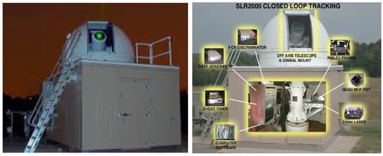
Figure 1.
The prototype NASA SLR2000 system projected a 2 kHz train of low energy, 532 nm, sub-nanosecond pulses via an unobscured 30 cm primary lens in order to concentrate more photons on the satellite while simultaneously eliminating potential eye hazards.
A quadrant Multi-Channel PhotoMultiplier Tube was used to keep the received signal centered in the detector. NASA funding for the actual construction of the SLR2000 prototype began in 1997. I initially named the system “SLR2000” for two reasons: (1) the prototype was expected to be operational shortly after the start of the new millennium, and (2) the laser fire rate was increased (coincidentally) from typically less than 10 pulses per second for NASA legacy systems to 2000 pulses per second. I retired from NASA in late 2002 to join Sigma Space Corporation in Lanham, MD USA as Chief Scientist and turned over leadership of the SLR2000 program to my highly competent colleague, Jan McGarry. Later in 2003, SLR2000 successfully tracked the US TOPEX-Poseidon satellite and was renamed Next Generation Satellite Laser Ranging (NGSLR) by NASA management. NGSLR continued to operate successfully until a lightning bolt destroyed it a few years later. Three copies of an upgraded successor system, the NASA Space Geodesy Satellite Laser Ranging System (SGSLR), are expected to begin operations at three locations by 2025, i.e., GSFC in Maryland USA, the McDonald Observatory in Texas USA, and the island of Ny Alesund in Norway [9].
3. NASA Multikilohertz Microlaser Altimeter (MMLA): The First Airborne Single Photon Lidar
While examining early SLR2000 data with my NASA colleague, Jan McGarry, I noticed that a plot of measured satellite range vs predicted range exhibited a linear slope as opposed to the expected horizontal line. When I questioned Jan about the cause of the discrepancy, she replied that it was due to a time bias in the predicted orbit. This triggered the following thought: “If I can see a slope in single photon satellite data due to a time bias, why can’t I see a real surface slope with a photon-counting lidar?”.
NASA agreed to fund the MMLA prototype via its Instrument Incubator Program. The Civil Service team included myself, Jan McGarry, and two engineering colleagues, Thomas Zagwodzki, and Phil Dabney, along with supporting contractors from Honeywell and the newly formed Sigma Space Corporation. The MMLA or “MicroAltimeter” was largely based on SLR2000 technology and successfully measured the times-of-flight of individual photons to deduce the distances between the instrument reference and points on the underlying terrain from which the arriving photons were reflected [14]. By imaging the terrain onto a highly pixelated detector followed by a multi-channel timing receiver, one can make multiple spatially resolved range measurements of the surface via a single laser pulse. The horizontal spatial resolution is limited by the optical projection of a single pixel onto the surface. In short, a 3D image of the terrain within the laser ground spot is obtained on each laser fire, assuming at least one signal photon is recorded by each pixel/timing channel. The passively Q-switched microchip Nd:YAG laser transmitter used in MMLA measured only 2.25 mm in length and was pumped by a single 1.2 Watt GaAs laser diode. The output was frequency-doubled to take advantage of the narrower beam divergence out of the telescope as well as the higher detector counting efficiencies and narrower spectral filters available at the 532 nm wavelength. The transmitter typically produced a few microjoules of green energy in a sub nanosecond pulse at several kilohertz rates. The illuminated ground area was imaged by a diffraction-limited, off-axis telescope onto an ungated, segmented anode photomultiplier with 16 pixels (4 × 4). The effective receive aperture was about 13 cm. Each anode segment was input to one channel of a “fine” range receiver (5 cm detector-limited resolution), which recorded the times-of-flight of the individual photons. A parallel “coarse” receiver provided a lower resolution (>75 cm) histogram of atmospheric scatterers and centered the “fine” receiver gate on the previous set of returns, thereby permitting the fine receiver to lock onto ground features with no apriori range knowledge. In test flights, the system operated successfully at mid-day at aircraft altitudes up to 6.7 km (22,000 ft), with single pulse laser output energies of only a few microjoules. It also recorded kHz single photon returns from clouds, soils, man-made objects, vegetation, and water surfaces. The system also demonstrated a capability to resolve volumetrically distributed targets, such as tree canopies and the underlying terrain, and successfully performed wave height measurements and shallow water bathymetry over the Chesapeake Bay and Atlantic Ocean. The temporally correlated signal photons were reliably extracted from the random solar and/or detector noise background using an optimized post-detection algorithm.
4. Single Photon Lidar Development at Sigma Space Corporation
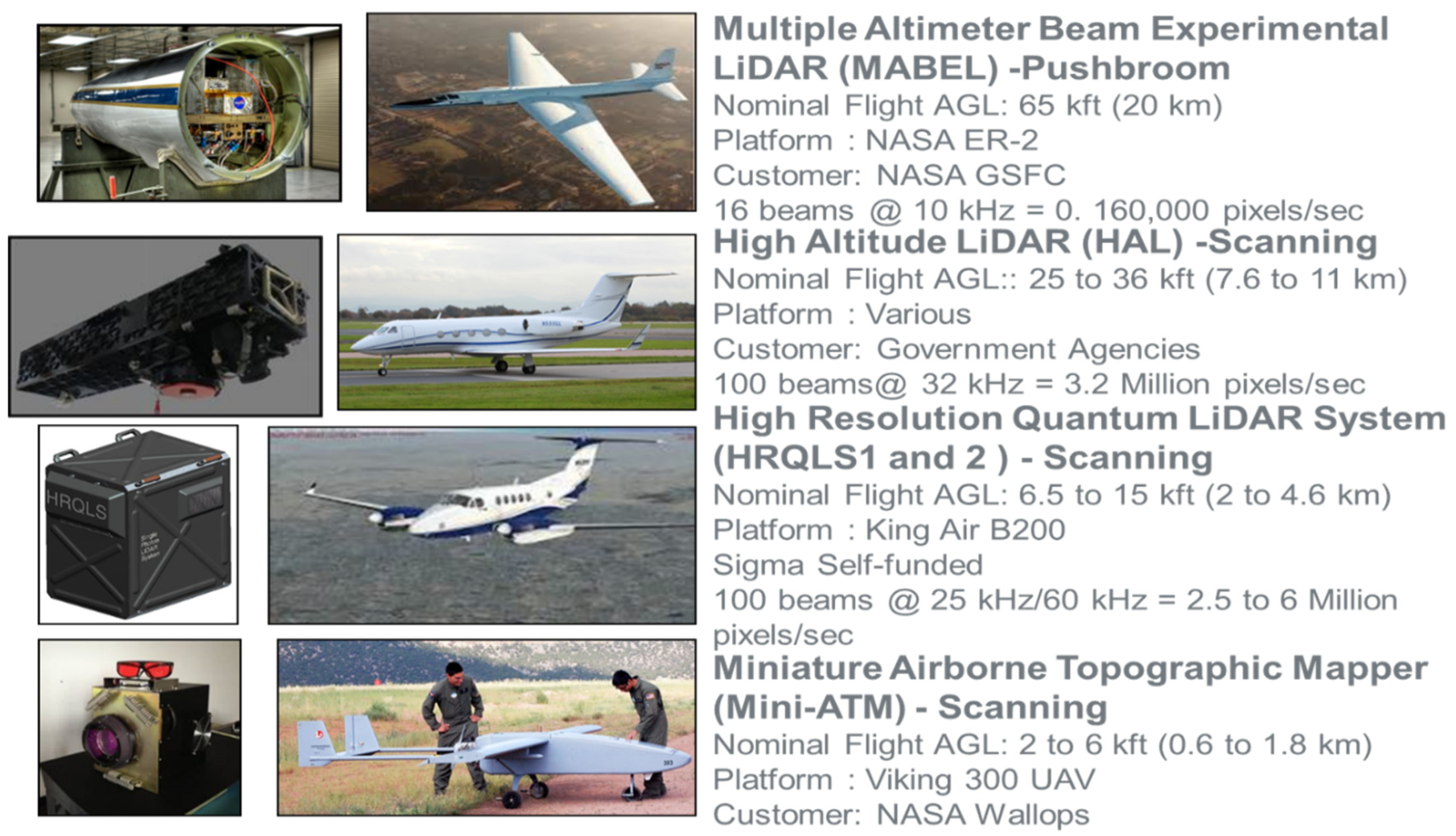
In early 2003, I retired from my 38-year career as a civil servant at NASA GSFC to take a position as Chief Scientist at Sigma Space Corporation, a relatively new corporation founded by Dr. Marcos Sirota and Joseph Marzouk. Sigma Space and Honeywell had provided contractor support to the MMLA Project, and Sigma was greatly interested in the further development of Single Photon Lidars (SPLs) for the commercial market. Over the next 15 years, Sigma introduced a variety of airborne single-photon-sensitive lidars, as summarized in Figure 2. The latter figure is excerpted from a comprehensive review article on Sigma’s SPL technology [15].
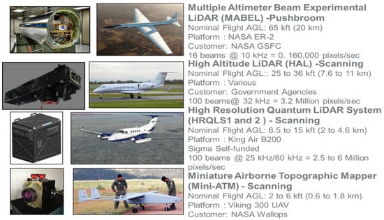
Figure 2.
Summary of airborne single photon lidars developed at Sigma Space Corporation.
The airborne Multiple Altimeter Beam Experimental Lidar (MABEL) at the top of Figure 2 was a 16 beam pushbroom lidar developed by Sigma for NASA as a testbed for the proposed ICESat-2 mission to be discussed in the next section. The High Altitude Lidar (HAL) and High Resolution Quantum Lidar System (HRQLS or “Hercules”), on the other hand, were scanning lidars designed for high spatial resolution, 3D imaging from high altitude aircraft. In the latter instruments, the laser beam was split into a 10 × 10 array of 100 beamlets via a dffractive element whose returns were imaged onto a matching 10 × 10 array of single photon sensitive detectors, such as a 10 × 10 segmented anode MicroChannel Plate PhotoMultiplier Tube (MCP/PMT) or a 10 × 10 Single Photon Avalanche Diode (SPAD) array.
Scanning was accomplished using the optical wedge scanner in Figure 3. A rotating single wedge traces a circle on the land surface. Over longer ranges at high altitudes, the receiver array FOV can become displaced along the circumference of the circle from the array of laser spots on the surface. To restore the overlap, we must add a “compensator wedge” which deflects the receiver FOV (or transmitter FOV but not both) at approximate right angles to the scanner wedge deflection. The Sigma Space lidars use an annular compensator wedge in which the transmitted laser beams pass unaffected through the small central hole while the receiver array FOV is angularly displaced opposite to the direction of rotation so that the detector array views the illuminated area as illustrated in Figure 3.
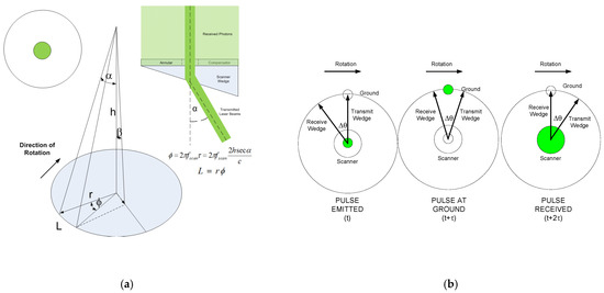
Figure 3.
A rotating single wedge traces a circle on the terrain. Over longer ranges, the receiver array FOV will, due to the finite speed of light, become displaced along the circumference of the circle from the array of laser spots on the surface. Therefore, we often use an annular compensator wedge in which the transmitted laser beamlets pass unaffected through a small central hole and are deflected by the optical wedge (a) while the receiver array FOV is angularly displaced opposite to the direction of rotation so that the detector array is viewing the illuminated area when the photons return from the surface (b).
Finally, photons reflected from the underlying terrain are spatially correlated but mixed with random photons due to solar illumination of the surface and/or intervening atmosphere as well as possible electronic noise in the receiver. The author previously developed an equation [16] for solar noise given by
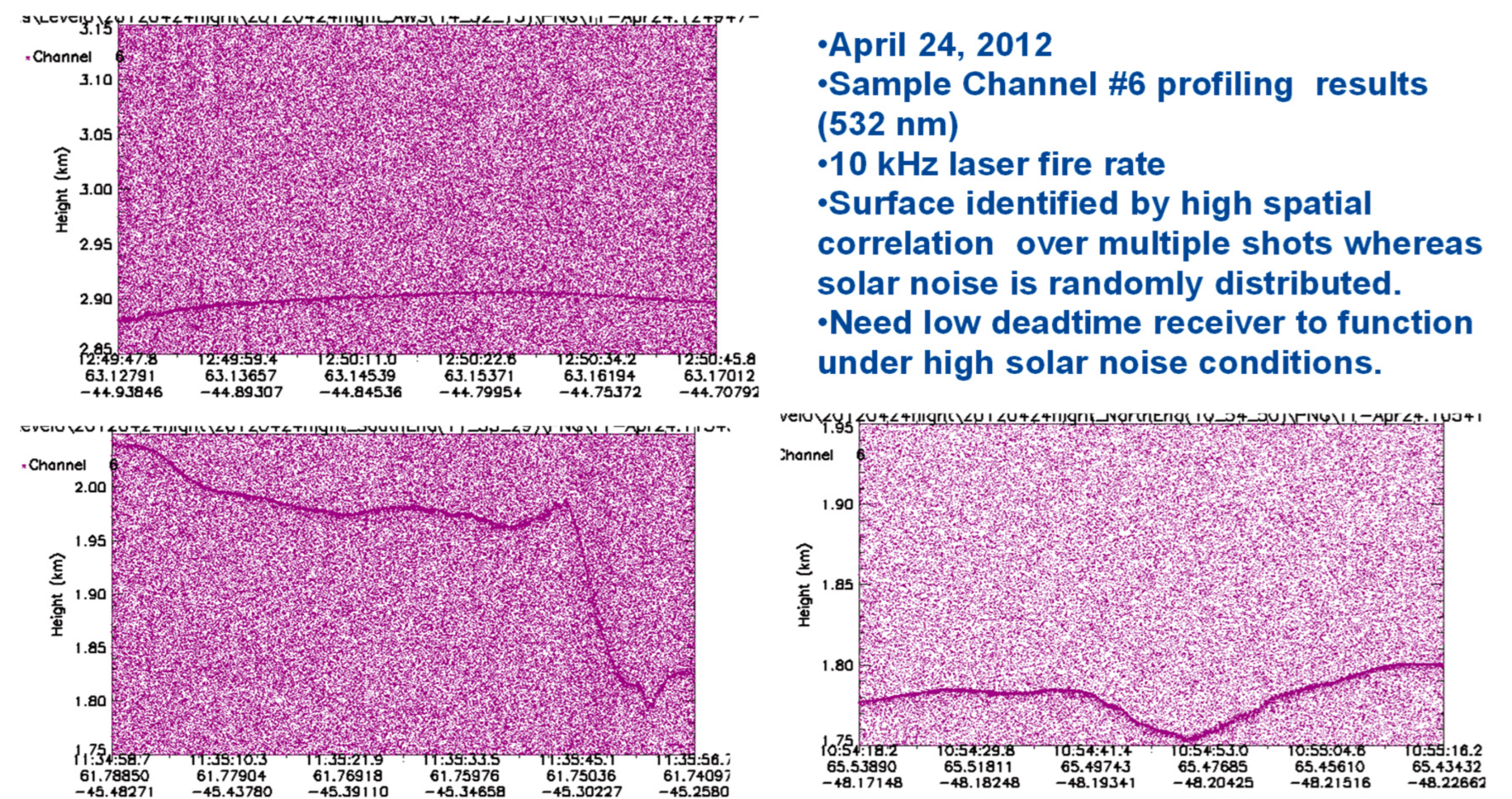
where Nλ0 = 0.2W/m2 Angstrom is the extraterrestrial solar irradiance impinging on the Earth’s atmosphere at the 532 nm laser wavelength, ηq is the detector efficiency, ηr is the receiver optical efficiency, hν is the laser photon energy, Ar is the area of the collecting telescope, T is the one way transmission of the atmosphere at zenith, ρ is the surface reflectance at the laser wavelength, θs is the solar zenith angle, ψ is the angle between the surface normal and the Sun, and Δλ and Ωr are the widths of the spectral and spatial filters. Thus, to obtain a clear 3D image of the surface, the receiver must have minimal deadtime between events and noise rejection software must be applied to the collected data. Typically, a two or three stage filter is used, i.e., one to reject the vast majority of noise relatively far from the surface followed by additional filtering to reject noise spatially intermingled with the surface returns. An example of this approach is shown in Figure 4 and final noise-edited images are provided in Figure 5, Figure 6 and Figure 7. Figure 8 provides sample data taken over Greenland in daylight from one beamlet (#6) of the 16 beamlet airborne pushbroom lidar MABEL The latter systemwas built to simulate the original 16 beamlet lidar proposed as a demonstration mission for ICESat-2. The figure clearly shows the ability of the lidar to distinguish the terrain from the background solar radiation over a wide range of slopes.
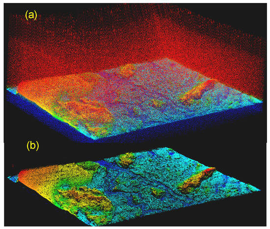
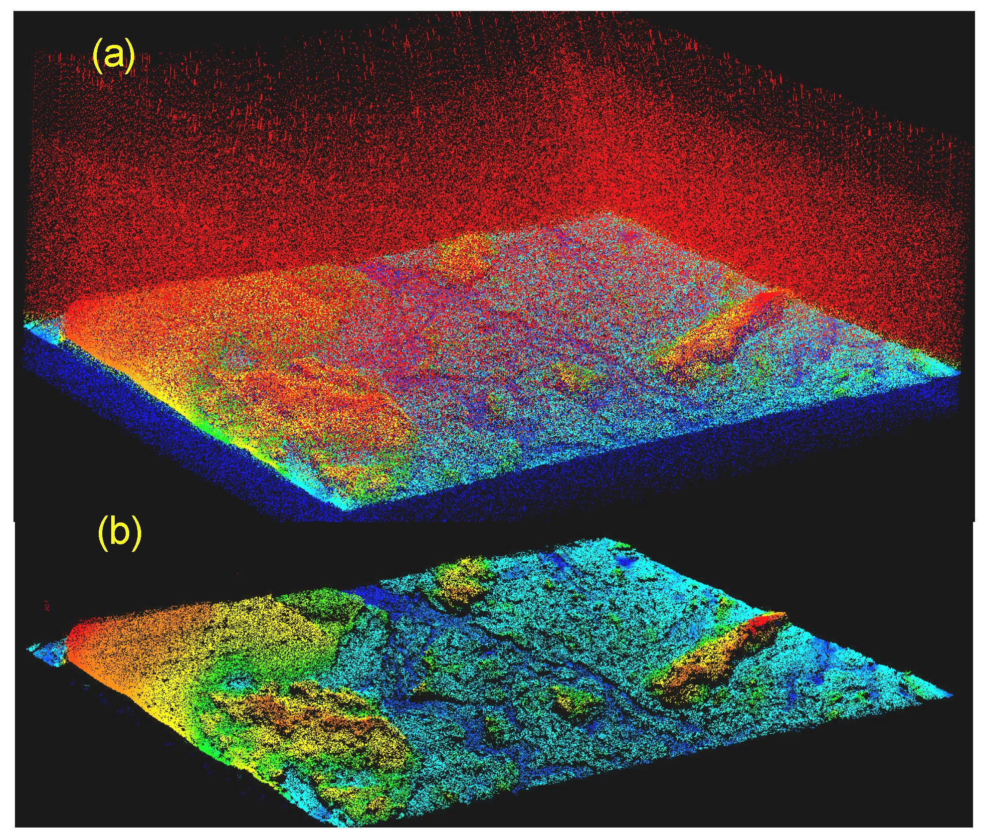
Figure 4.
Editing Noise (a) Unedited point cloud of Greenland terrain (surface reflectivity > 0.9) shows a fair amount of solar noise above (red haze) and below (blue haze) the surface. (b) same point cloud image after use of Sigma-developed noise-editing filters.
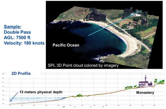
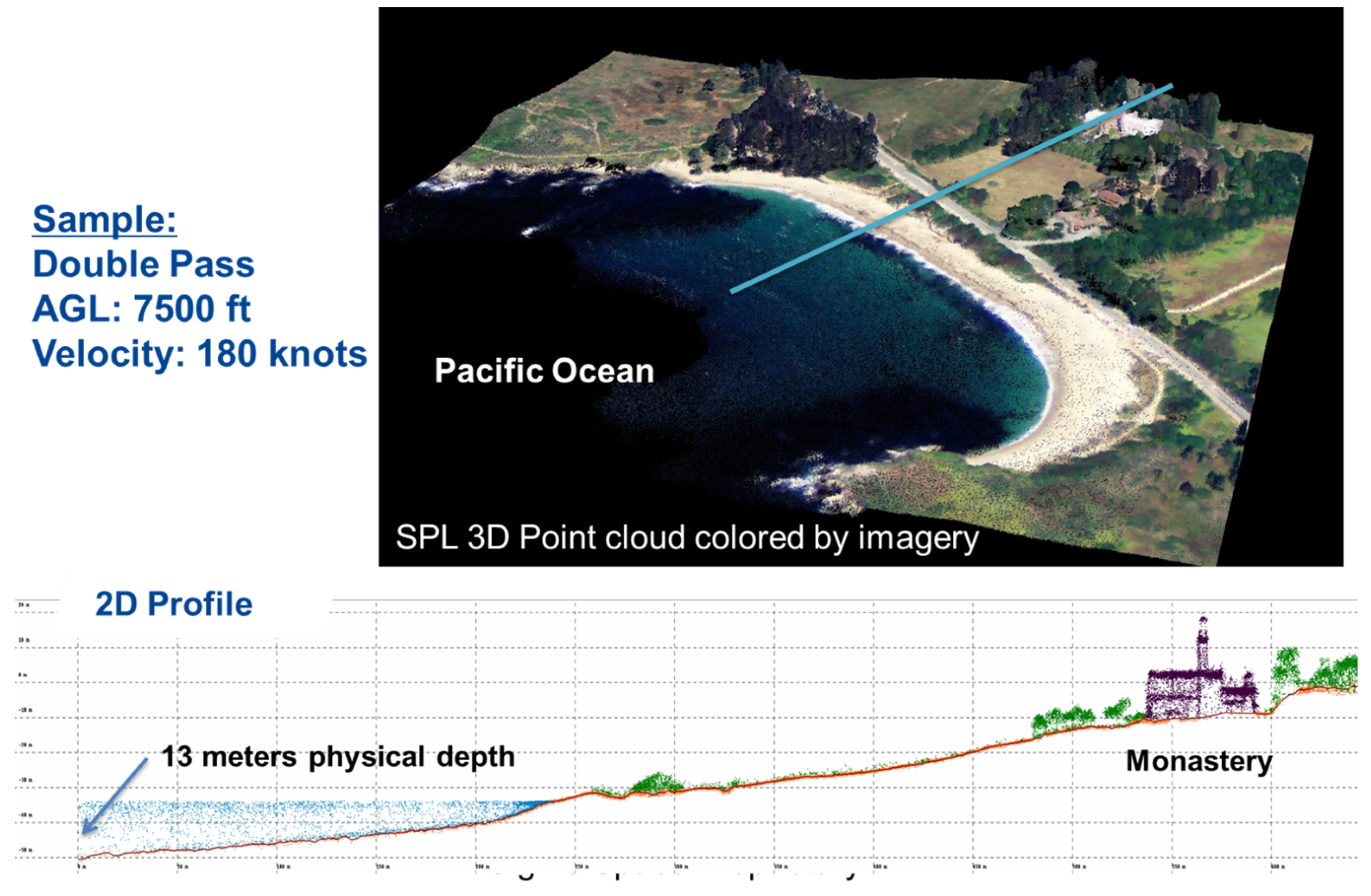
Figure 5.
(Top) Lidar image of the Pacific coastline in Port Lobos, California. (Bottom) Detailed look along the blue line in the top figure showing a hilltop monastery, the heights of various trees, the surface of the Pacific Ocean, and the ocean bottom to a depth of 13 m (42.7 ft).
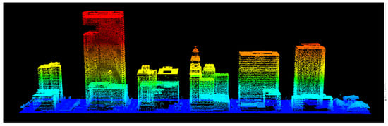
Figure 6.
Single photon lidar image of downtown Houston, Texas, taken by the Sigma HRQLS system (pronounced “Hercules”). Colors were arbitrarily assigned based on height above the ground.
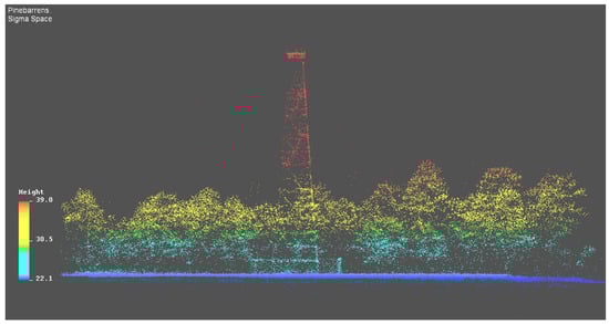
Figure 7.
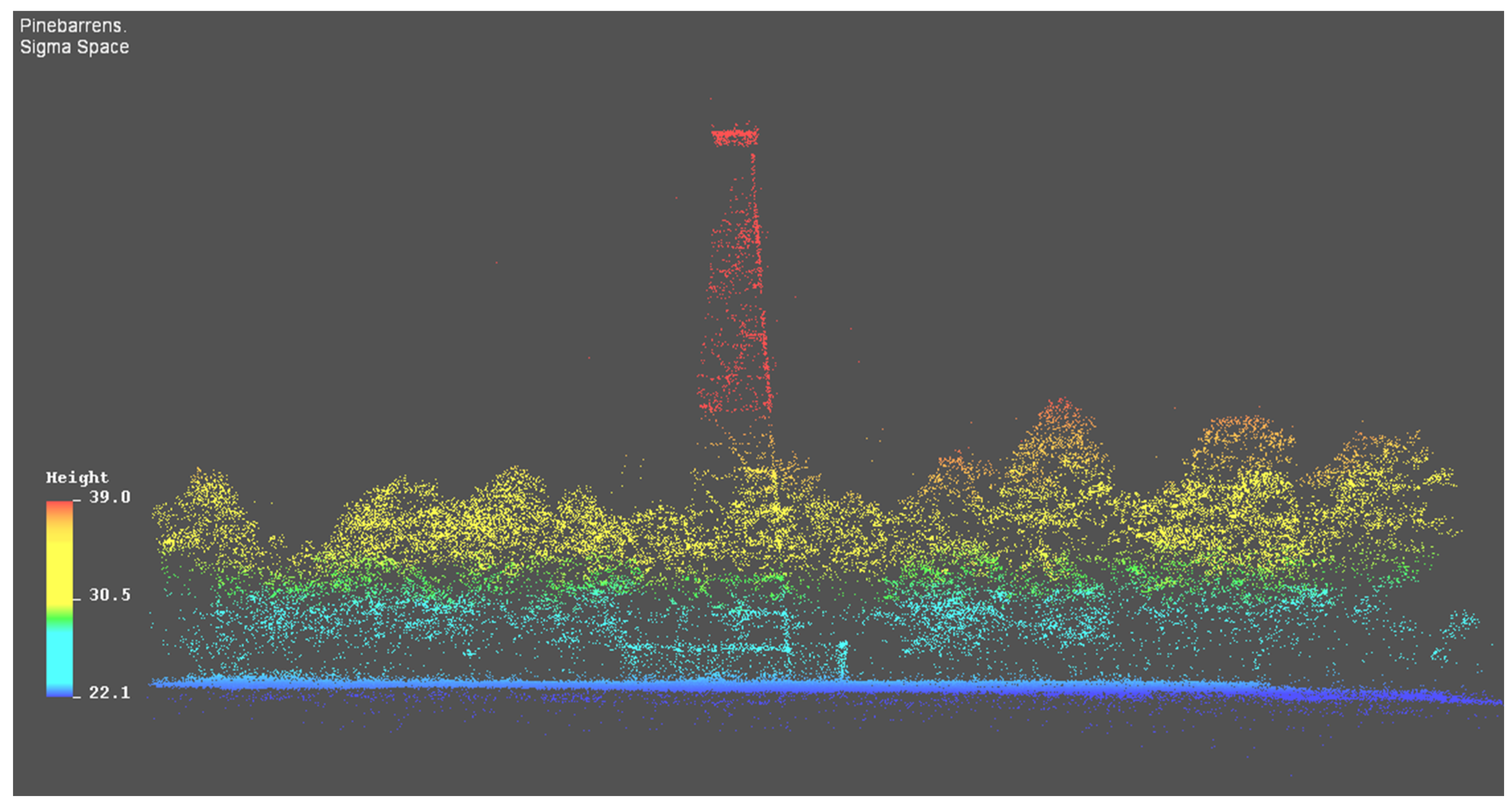
Side view of an airborne 3D image of a fire tower surrounded by a chain link fence and trees of varying height. Colors are arbitrarily assigned based on height above the surface.
The success of the high altitude airborne SPLs, designed and manufactured by Sigma Space Corporation, clearly demonstrated the amazing detail that could be obtained over a wide variety of landscapes. These included rural and forested areas [17], tall city buildings, homes, and other manmade structures, rugged and sloped terrain, ice floes, power lines, and the surface and bottoms of shallow water bodies with depths up to several tens of meters.
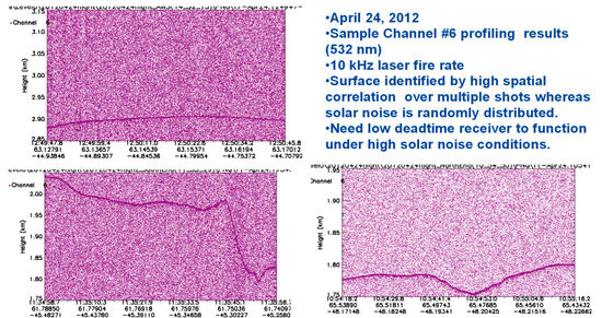
Figure 8.
Sample surface data from a single channel (#6) of the 16-channel airborne MABELpush-broom lidar taken over the Greenland ice sheet from an altitude of 20 km [18]. The data demonstrated the lidar’s ability to observe a wide range of surface slopes in the presence of high-intensity solar (or detector) noise due to high spatial correlation of the surface counts and a low deadtime receiver.
5. Configuring the ICESat-2 Single Photon Lidar
NASA had previously flown multiple spaceborne multiphoton lidars, including the following:
- the Mars Orbiter Laser Altimeter (MOLA) from 1997 to 2001;
- the GLAS (Geoscience Laser Altimeter System) on ICESat-1 about the Earth from 2003 to 2009;
- the MESSENGER mission to Mercury from 2011 to 2015;
- and the Lunar Observer Laser Altimeter (LOLA) about the Moon from 2009 to the present.
The aforementioned multiphoton spaceborne lidars operated at a few tens of pulses per second, and it rapidly became clear to the author that spaceborne SPL technology could be more lightweight, less complex, and provide orders of magnitude more surface data, especially in orbit about planets or moons with less atmosphere and surface diversity than Earth [16].Therefore, in 2006, I gave several presentations to the NASA ICESat-2 Project team at Goddard Space Flight Center. The presentations outlined the potential benefits of a multibeam, single photon lidar in Earth orbit. The original design presented a single 5 Watt, actively Q-switched, frequency doubled, subnanosecond pulse Nd:YAG microlaser operating at the 532 nm wavelength and generating a train of 500 microjoule pulses at a rate of 10 kHz. The beam would then be split into 16 equally spaced, 310 mW beamlets distributed along a line perpendicular to the satellite flight path. Thus, the proposed configuration was designed to generate 160,000 surface measurements per second compared to only 40 measurements per second for the predecessor GLAS single beam, multiphoton lidar flown on ICESat-1. In addition, the green wavelength would permit some degree of penetration in water bodies for bathymetric measurements.
Initially, the ICESat-2 project team saw potential merit in the SPL approach and proposed to fly a copy of the earlier GLAS system along with an experimental version of the proposed 16 beam SPL on the ICESat-2 mission. However, budget problems later forced the Project to abandon the dual lidar concept. Fortunately, results from the NASA-funded airborne version of Sigma’s 16 beam pushbroom SPL, MABEL, helped to bolster confidence in the technique as illustrated in Figure 8 [18]. Nevertheless, it was not yet entirely clear that the 16 beam lidar proposed by Sigma could meet all of the science requirements of the mission.
Ultimately, the Project chose a modified version of my proposed single photon lidar which consisted of 3 “strong” and 3 “weak” beams for reasons to be described shortly. The strong beams would each contain roughly four times the pulse energy (2 mJ) of one of the original 16 weak beams thereby reducing the surface sampling rate from 160,000 measurements per second to 60,000 per second but still representing a factor of 1500 increase in potential surface detection rate relative to the original GLAS system on ICESat-1.
In order to reach this final instrument configuration, I again collaborated with my longtime NASA colleague and subsequent ICESat-2 Algorithm Lead, Jan McGarry, to assess the performance of various beam strengths for each of the 13 measurement scenarios in Table 1. I devised a Differential Cell Count (DCC) approach while Jan suggested a Noise Only (NO) method for extracting the weak surface signal from solar background noise over the range of measurement scenarios which were considered critical by the ICESat-2 Project Science Team. As outlined in Table 1, these scenarios included cryosphere, biomass, and ocean measurements. Furthermore, successful measurements were desired for terrain slopes up to 45 degrees. In the process, we each used lidar link analyses and solar noise models appropriate for each of the 13 measurement scenarios provided by the science team and optimized the size of the range bin. The number of beamlets and their powers were also varied, keeping the overall laser power constant, in order to determine their compatibility with the measurement goals.

Table 1.
The ATLAS science team identified 13 measurement scenarios crucial to their overall mission, including six ice-related scenarios (1a through 6a), three tree penetration scenarios (8a, 9a, and 10a), and three wind measurements (10a, 10b, and 10c). The expected signal counts and noise rates for each scenario are listed in the final two columns of the table.
Table 2 is extracted from a PowerPoint presentation by the author to the ICESat-2 science team in December 2011. As can be seen from the far left column in Table 2, four different combinations of beam strengths were considered: (1) 16 equal weak beams (as originally proposed by the author for the test flight configuration); (2) 6 equal beams each containing 2.5 times the energy in the original weak beam; (3) 5 equal beams each containing 3 times the energy in the weak beam; and (4) strong beams each containing 4 times the energy in the weak beam. In turn, each of these categories were further divided into two elements depending on which detection algorithm was being used, i.e., the Differential Cell Count (DCC) or Noise Only (NO) method. Dark blue color indicates excellent performance, dark green signifies very good, with light green, yellow, orange, and red indicating increasingly degraded performance in each measurement category. To summarize, the three strong beams perform well in all of the measurement scenarios while the remaining 3 weak beams can double the measurement density in certain science categories such as 1a, 8a, and 10a. The above conclusions were considered conservative by the Science Team since the calculations assumed, for simplicity, a worst case where the surface photons are distributed uniformly in time by either a constant slope within the frame or the tree canopy which they are not.
Table 2.
Summary of beam strength performance for the 13 ICESat-2 science goals.
6. Summary
As described herein, the precision ranging capability of the current ATLAS lidar relied heavily on almost four decades of relevant experience in Satellite Laser Ranging (SLR) during which the ranging precision improved from 2 m to a few millimeters. Subsequently, the growing international science and engineering demands for precise satellite ranging at a lower manufacturing and operational cost resulted in NASA’s development of the single photon sensitive SLR2000 system. The latter design drew heavily from early NASA laser space communication studies of optical antenna gain conducted in the 1970s. These studies advocated for the use of a single telescope to (1) transmit the pulse in a significantly less divergent beam (thereby placing an orders of magnitude higher fraction of the transmitted laser pulse energy on the target), and (2) capturing some of the energy reflected by the satellite retroreflectors. This innovation not only significantly reduced the size and cost of the optical telescope, tracking mount, and shelter, but it also greatly reduced the required laser pulse energy. Thus, the large, complex, expensive, and low repetition rate modelocked lasers could be replaced by relatively inexpensive, compact, low energy, actively or passively Q-switched microchip lasers producing tens of thousands of subnanosecond pulses per second.
In this paper, the author has attempted to describe for the reader the highly complicated technical path which ultimately led NASA researchers and their contractors to the highly successful ATLAS Multibeam Single Photon Lidar (SPL). The latter instrument was launched, in September 2018, aboard the ICESat-2 spacecraft into a roughly 500 km high orbit about the Earth. At that altitude, the six beams and 10 kHz laser pulse rate permit a total of 60,000 surface measurements per second and surface measurements every 70 cm along the flight path for each of the 6 beamlets. The ICESat-2 science goals included few cm accuracy topographic measurements over land, ice, and sea surfaces as well as tree canopy and cloud heights.
The ATLAS lidar includes an 80 cm diameter telescope which can redirect the beams. An initial evaluation of ATLAS performance published in 2021, after more than one trillion surface measurements had been made, concluded with the following statement. “The ICESat-2 geolocated photons show a horizontal position accuracy of 3.6 m (1 σ) over both long length scales and through local validation, and a vertical accuracy of better than 10 cm” [19]. A wide range of publications reporting on the ICESat-2 instrument and data analyses can be found on a routinely updated NASA website at https://icesat-2.gsfc.nasa.gov (accessed on 1 September 2024).
Funding
This research received no external funding.
Data Availability Statement
The original contributions presented in the study are included in the article, further inquiries can be directed to the corresponding author.
Conflicts of Interest
The authors declare no conflict of interest.
References
- Maiman, T.H. Optical Radiation in Ruby. Nature 1960, 187, 493–494. [Google Scholar] [CrossRef]
- Plotkin, H.H.; Johnson, T.S.; Spadin, P.; Moye, J. Reflection of Ruby Laser Radiation from Explorer XXII. Proc. IEEE 1965, 53, 301–302. [Google Scholar] [CrossRef]
- Alley, C.O.; Chang, R.; Currie, D.; Mullendore, J.; Poltney, S.; Rayner, J.D.; Silverberg, E.; Steggerda, C.; Plotkin, H.; Williams, W.; et al. Apollo 11 Laser Ranging Retroreflector: Initial Measurements from the McDonald Observatory. Science 1970, 167, 368–370. [Google Scholar] [CrossRef]
- Degnan, J.J. Millimeter Accuracy Satellite Laser Ranging: A Review. Contrib. Space Geod.Geodyn. Technol. 1993, 25, 133–162. [Google Scholar]
- Degnan, J.J. A Tutorial on Retroreflectors and Arrays Used in Satellite and Lunar Laser Ranging. Photonics 2023, 10, 1215. [Google Scholar] [CrossRef]
- Nicolas, J.; Pierron, F.; Kasser, M.; Exertier, P.; Bonnefond, P.; Barlier, F.; Haase, J. French transportable laser ranging station: Scientific objectives, technical features, and performance. Appl. Opt. 2000, 39, 402–410. [Google Scholar] [CrossRef] [PubMed]
- Pearlman, M.R.; Noll, C.E.; Pavlis, E.C.; Lemoine, F.G.; Combrinck, L.; Degnan, J.J.; Kirschner, G.; Schreiber, K.U. The ILRS: Approaching 20 Years and Planning for the Future. J. Geod. 2019, 93, 2161–2180. [Google Scholar] [CrossRef]
- Wilkinson, M.; Schreiber, K.U.; Prochazka, I.; Moore, C.; Degnan, J.J.; Kirchner, G.; Zhonping, Z.; Dunn, P.; Shargorodsky, V.; Sadovnikov, M.; et al. The Next Generation of Satellite Laser Ranging Systems. J. Geod. 2019, 93, 2227–2247. [Google Scholar] [CrossRef]
- McGarry, J.F.; Degnan, J.J.; Cheek, J.W.; Clarke, C.B.; Diegel, F.; Donovan, H.L.; Horvath, J.E.; Marzouk, M.; Nelson, A.R.; Patterson, D.S.; et al. NASA’s Satellite Laser Ranging Systems for the 21st Century. J. Geod. 2019, 93, 2249–2262. [Google Scholar] [CrossRef]
- Klein, B.J.; Degnan, J.J. Optical Antenna Gain 1: Transmitting Antennas. Appl. Opt. 1974, 13, 2134–2141. [Google Scholar] [CrossRef] [PubMed]
- Degnan, J.J.; Klein, B.J. Optical Antenna Gain 2: Receiving Antennas. Appl. Opt. 1974, 13, 2397–2401, Erratum in Appl. Opt. 1974, 13, 2762. [Google Scholar] [CrossRef] [PubMed]
- Degnan, J.J. Optimal Design of Passively Q-switched Microlaser Transmitters for Satellite Laser Ranging. In Proceedings of the 10th International Workshop on Laser Ranging, Shanghai, China, 11–15 November 1996; pp. 334–343. [Google Scholar]
- Degnan, J.J.; Zayhowski, J.J. SLR2000 Microlaser Performance: Theory and Experiment. In Proceedings of the 11th International Workshop on Laser Ranging, Deggendorf, Germany, 21–25 September 1998; pp. 453–468. [Google Scholar]
- Degnan, J.J.; McGarry, J.F.; Dabney, P.; Zagwodzki, T.W. Design and Performance of an Airborne Multi-kilohertz Photon-Counting Microlaser Altimeter. Int. Arch. Photogramm. Remote Sens. Spat. Inf. Sci. 2001, 34, 9–16. [Google Scholar]
- Degnan, J.J. Scanning, multibeam, single photon lidars for rapid, large scale, high resolution topographic and bathymetric mapping. Remote Sens. 2016, 8, 958. [Google Scholar] [CrossRef]
- Swatantran, A.; Tang, H.; Barrett, T.; DeCola, P.; Dubayah, R. High-Resolution Forest Structure and Terrain Mapping over Large Areas using Single Photon Lidar. Sci. Rep. 2016, 6, 28277. [Google Scholar] [CrossRef] [PubMed]
- Degnan, J.J. Photon-counting multikilohertz microlaser altimeters for airborne and spaceborne topographic measurements. J. Geodyn. 2002, 34, 503–549. [Google Scholar] [CrossRef]
- McGill, M.; Markus, T.; Scott, V.S.; Neumann, T. The Multiple Altimeter Beam Experimental Lidar (MABEL): An Airborne Simulator for the ICESat-2 Mission. J. Atmos. Ocean. Technol. 2013, 30, 345–352. [Google Scholar] [CrossRef]
- MacGrudor, L.; Neumann, T.; Kurtz, N. ICESat-2 Early Mission Synopsis and Observatory Performance. Earth Space Sci. 2021, 8, 5. [Google Scholar] [CrossRef] [PubMed]


Disclaimer/Publisher’s Note: The statements, opinions and data contained in all publications are solely those of the individual author(s) and contributor(s) and not of MDPI and/or the editor(s). MDPI and/or the editor(s) disclaim responsibility for any injury to people or property resulting from any ideas, methods, instructions or products referred to in the content. |
© 2024 by the author. Licensee MDPI, Basel, Switzerland. This article is an open access article distributed under the terms and conditions of the Creative Commons Attribution (CC BY) license (https://creativecommons.org/licenses/by/4.0/).