A Numerical Assessment of the Effect of Concatenating Arbitrary Uncoupled Multicore Fiber Segments on Intercore Crosstalk in Long-Haul Communication Links

Abstract

Random core dependent loss (CDL) has been shown to increase the direct average intercore crosstalk (ICXT) power in long-haul uncoupled multicore fiber (MCF) links. Longer links are composed of multiple MCF segments, and random CDL may arise on these links from manufacturing imperfections. During link implementation, other random effects may arise and enhance the ICXT power. In this work, the effect of concatenating MCF segments with random characteristics on the direct average ICXT power in long-haul links is assessed numerically by studying the influence of the randomness of segment length, coupling coefficient, and random CDL on the mean, standard deviation, relative spread, and excess kurtosis of the ICXT power. The numerical results show that the segment length randomness marginally affects the ICXT power. For 2000 km long links and a 6 dB maximum random variation of the coupling coefficients, the mean almost doubles and the standard deviation almost triples, relative to considering only random CDL. However, the effect of the coupling coefficients randomness on the relative spread and excess kurtosis is reduced, not affecting significantly the nearly Gaussian distribution of the direct average ICXT power and the excess of direct average ICXT power (less than a 0.26 dB increase relative to considering only random CDL).

1. Introduction

Although coupled core fibers are currently receiving research attention [1], uncoupled multicore fibers (MCFs) are seen as a promising solution to support space-division multiplexing in long-haul MCF links where the available physical space is limited, such as submarine cables [2,3,4] or even in shorter optical datacenter network links [5,6]. Long-haul terrestrial transmission links are typically composed of multiple spliced fiber segments (typically ~2 km in length) [7], which are taken from different lots [8]. As such, core dependent loss (CDL) due to manufacturing imperfections [9,10,11] may vary from MCF segment to MCF segment [8]. Moreover, in uncoupled MCF links with unidirectional transmission, intercore crosstalk (ICXT) may significantly impair the transmission performance [12,13]. The impact of CDL on the direct average ICXT power in two-core unsegmented uncoupled MCFs was studied theoretically [8,14]. It was concluded that the variation of the direct average ICXT power with constant CDL can reach up to 2 dB (for CDL in the range of ±0.04 dB/km) in comparison with MCFs with equal core losses [14]. In two-core uncoupled segmented MCF links, the impact of random CDL from different concatenated MCF segments on the direct average ICXT power was studied numerically and analytically [15]. We have shown [15] that (i) random CDL leads to probability density functions (PDFs) of the direct average ICXT power that are nearly Gaussian, as long as the number of concatenated MCF segments is sufficiently high and (ii) the arbitrariness of the MCF segments concatenation may reduce the CDL impact on the direct average ICXT power relative to unsegmented MCF links with constant CDL. Using an analytical worst-case approximation, it has been shown that random CDL leads only to a 0.25 dB excess of direct average ICXT power relative to its mean for 2000 km long links [15]. Shorter links will experience a higher excess of direct average ICXT power due to random CDL since less Gaussian PDF behavior observed for a lower number of concatenated segments enhances the relative spread of the direct average ICXT power [15].

When deploying the transmission link, variable splice loss can also enhance the direct average ICXT power [16,17]. The combined effect of CDL and splice loss on the direct average ICXT power has been studied in [16] for fixed loss values, and it was shown that its impact on the direct average ICXT power only depends on the total loss difference. The impact of the combined effect of random CDL and random splice loss on the direct average ICXT power in long-haul MCF links has been assessed in [17]. For splice loss practical values, it was shown that the effect of random splice loss dominates the excess of ICXT power, leading to 2 dB and 0.6 dB of excess power, respectively, for 100 km and 2000 km long links [17].

Other random effects resulting from imperfect fiber manufacturing, such as coupling coefficient variation along the MCF link [18], or resulting from link implementation issues, such as segment length variation, may, after segment concatenation, intensify and enhance the direct average ICXT power. The impact of such effects remains to be assessed and quantified. Hence, this work numerically assesses the combined effect of the randomness of the segment length, power coupling coefficient, and CDL on the statistical behavior of the direct average ICXT power, namely, on its PDF, mean, standard deviation, relative spread, and excess kurtosis and on the induced excess of direct average ICXT power.

The remainder of this paper is organized as follows. Section 2 describes the numerical model of the MCF link, the theory, and the corresponding equations used to calculate the direct average ICXT power at the link output. In Section 3, the numerical results regarding the direct average ICXT power are obtained, statistically studied, and discussed. The main conclusions are presented in Section 4.

2. Numerical Model

This section describes the numerical model used to study the effect of concatenating arbitrary MCF segments with different characteristics on the statistical behavior of the direct average ICXT power in long-haul communication links. The equivalent model of the k-th span is depicted in Figure 1 and closely follows the model proposed in [15]. Each uncoupled MCF link comprises N_s spans, with the span length denoted as L_s,k (with k = 1, …, N_s). At the end of each MCF span, a multicore-optical amplifier (MC-OA) compensates for the span loss. Each span is composed of N_k concatenated MCF segments interconnected by splice points (totaling N_k − 1 in the k-th span), with the segment length denoted as L_i,k (with i = 1, …, N_k). The total length of the k-th span is $L_{s,k}={\displaystyle {\sum }_{i=1}^{N_k}{L}_{i,k}}$.

The power at the output of the k-th span, P_out,c,k (with c = 1 for core 1 and c = 2 for core 2), is obtained using [15] the following:

$$\left[\begin{array}{c}{P}_{out,1,k}\\ P_{out,2,k}\end{array}\right]=T_{OA,k}{T}_{N_k,k}{C}_{N_k-1,k}{T}_{N_k-1,k}\cdots C_{2,k}{T}_{2,k}{C}_{1,k}{T}_{1,k}\left[\begin{array}{c}{P}_{in,1,k}\\ P_{in,2,k}\end{array}\right]$$

(1)

where P_in,c,k (with c = 1 or 2) denotes the power at the input of the k-th span. Each matrix T_i,k (with i = 1, …, N_k and k = 1, …, N_s), as given by (2), represents the coupled power equations with CDL between cores 1 and 2 in the i-th MCF segment of the k-th span [8].

$$\begin{array}{l}{T}_{i,k}=\exp \left[-\left({\overline{\alpha }}_{i,k}+h_{i,k}\right)L_{i,k}\right]\cdot \\ \cdot \left[\begin{array}{cc}\cosh \left({\eta }_{i,k}{L}_{i,k}\right)-{\delta }_{\alpha ,i,k}{L}_{i,k}\cdot {\displaystyle \frac{\sinh \left({\eta }_{i,k}{L}_{i,k}\right)}{{\eta }_{i,k}{L}_{i,k}}}& h_{i,k}{L}_{i,k}{\displaystyle \frac{\sinh \left({\eta }_{i,k}{L}_{i,k}\right)}{{\eta }_{i,k}{L}_{i,k}}}\\ h_{i,k}{L}_{i,k}{\displaystyle \frac{\sinh \left({\eta }_{i,k}{L}_{i,k}\right)}{{\eta }_{i,k}{L}_{i,k}}}& \cosh \left({\eta }_{i,k}{L}_{i,k}\right)+{\delta }_{\alpha ,i,k}{L}_{i,k}\cdot {\displaystyle \frac{\sinh \left({\eta }_{i,k}{L}_{i,k}\right)}{{\eta }_{i,k}{L}_{i,k}}}\end{array}\right]\end{array}$$

(2)

$${\eta }_{i,k}={\left(h_{i,k}^2+{\delta }_{\alpha ,i,k}^2\right)}^{1/2}$$

(3)

where h_i,k is the power coupling coefficient between the two cores in the i-th segment of the k-th span (we assume that h_12,i,k ≈ h_21,i,k = h_i,k, which is valid in the practical range of CDL [8,14]); ${\overline{\alpha }}_{i,k}$ is the average of the loss coefficients of the two cores in the i-th segment of the k-th span and is given by ${\overline{\alpha }}_{i,k}$ = (α_1,i,k + α_2,i,k)/2, where α_c,i,k (with c = 1 or 2) corresponds to the loss coefficient of core c in the i-th segment of the k-th span; and ${\delta }_{\alpha ,i,k}$ = (α_1,i,k − α_2,i,k)/2, with the loss coefficient imbalance defined by 2${\delta }_{\alpha ,i,k}$ and corresponding to CDL [8].

As MCF segments can come from different lots, due to manufacturing imperfections, the MCF segments may exhibit different characteristics, such as different lengths, coupling coefficients, and CDL. CDL ranges of [−0.04, 0.04] dB/km have been reported [11]. It is also very unlikely that CDL will be more than 0.1 dB [8]. As CDL between segments can be (arbitrarily) different, the CDL in the i-th each segment may be characterized as a random variable (RV) by assuming that the loss coefficients in the i-th MCF segment are also RVs. A statistical distribution is assumed to characterize random CDL, where the loss coefficients α_c,i,k can only assume two values with a probability of ½. The PDF of this distribution is given by [15] the following equation:

$$p\left(x\right)={\displaystyle \frac{1}{2}}\delta \left(x-{\alpha }_{c,min}\right)+{\displaystyle \frac{1}{2}}\delta \left(x-{\alpha }_{c,max}\right)$$

(4)

where δ(x) stands for the Dirac delta function. It should not be confused with the variable δ_α,i,k that characterizes the loss coefficient imbalance. The two values α_c,min and α_c,max correspond to, respectively, the minimum and maximum loss coefficients that can be set in each MCF segment. It has been shown that the distribution given by (4) is a worst-case distribution that enhances the impact of random CDL on the direct average ICXT power at the output of the MCF link relative to other statistical distributions [15]. The work reported in [15] assumed that the power coupling coefficient is equal for all segments and that all segments have the same length.

The coupling coefficients between cores in each MCF segment and the segment lengths are also modeled as RVs. The power coupling coefficient in the i-th segment of the k-th span is generated uniformly in the interval $h_{i,k}=\left[{10}^{-V_h[\mathrm{dB}]/10}\cdot h_{ref},{10}^{V_h[\mathrm{dB}]/10}\cdot h_{ref}\right]$, where V_h sets the maximum variation, in dB, of the power coupling coefficient relative to the reference case h_ref. The length of the i-th segment of the k-th span is generated uniformly in the interval $L_{i,k}=\left[\left(1-{\Delta }_L\right)\cdot L_{ref},\left(1+{\Delta }_L\right)\cdot L_{ref}\right]$, where ${\Delta }_L$ sets the maximum fractional variation of the segment length relative to the reference case L_ref. This approach to study the effect of the segment length randomness on the direct average ICXT power follows the idea presented in [19] for studying randomly variable map lengths in dispersion-managed links. We also assume that the random effects in each segment are considered independent of the random effects of other segments.

The MCF segments are interconnected by splices created during the construction of the MCF link. At each splice point, the matrices C_i,k (with i = 1, …, N_k − 1 and k = 1, …, N_s) in Equation (1) are given by [16] the following equation:

$$C_{i,k}=\left[\begin{array}{cc}{\eta }_{11,i,k}& {\eta }_{12,i,k}\\ {\eta }_{21,i,k}& {\eta }_{22,i,k}\end{array}\right]$$

(5)

where η_cc,i,k (with c = 1 or 2) defines the loss of the splice point for core c in the i-th segment of the k-th span and η_cc’,i,k (with c’ ≠ c) defines the mode coupling between the two cores at the i-th splice point of the k-th span. The splice loss difference definition considered in [16] can be used to set the loss of each splice point. Additionally, the matrices C_i,k in Equation (5) are typically diagonal matrices, since the ICXT caused by mode coupling at the splice point is usually low when compared to the MCF-induced ICXT [16].

An investigation regarding how random splice loss affects the direct average ICXT power in long-distance transmission was performed in [16,17]. Due to its high magnitude, splice losses may dominate the ICXT power enhancement and may conceal the impact of the coupling coefficient randomness and segment length randomness on such enhancement. To avoid this situation, in the remainder of this work, we consider that the splices have equal losses in the two cores and along the long-haul MCF link.

After N_k MCF segments, an ideal MC-OA perfectly compensates the optical loss in each core. As the main goal of this work is to study the effect of concatenating arbitrary MCF segments on the direct average ICXT power, the noise of the amplifiers is neglected. The gain of each core is equal to the overall loss of the k-th span, with the diagonal matrix T_OA,k in Equation (1) defined by

$$T_{OA,k}=\left[\begin{array}{cc}\exp \left({\displaystyle {\sum }_{i=1}^{N_k}{\alpha }_{1,i,k}{L}_{i,k}}\right)& 0\\ 0& \exp \left({\displaystyle {\sum }_{i=1}^{N_k}{\alpha }_{2,i,k}{L}_{i,k}}\right)\end{array}\right], \mathrm{with} k=1, \dots , N_s$$

(6)

where the mode coupling in the MC-OAs is assumed to be negligible in comparison with the ICXT induced by the MCF.

At the output of the long-haul MCF link with total length L_tot, the optical power in each core is calculated using

$$\left[\begin{array}{c}{P}_{out,1,N_s}\\ P_{out,2,N_s}\end{array}\right]=T_{OA,N_s}{T}_{N_{N_s},N_s}{C}_{N_{N_s}-1,N_s}\cdots C_{1,N_s}{T}_{1,N_s}\cdots T_{OA,1}{T}_{N_1,1}{C}_{N_1-1,1}\cdots C_{1,1}{T}_{1,1}\left[\begin{array}{c}{P}_{in,1,1}\\ P_{in,2,1}\end{array}\right]$$

(7)

The direct average ICXT power, XT_dir, in core c (with c = 1 or 2), after N_s spans, at the output of the long-haul MCF link is obtained by [14] the following equation:

$$X{T}_{dir,c}=P_{cou,c}\left(L_{tot}\right)/P_{sig,c}\left(L_{tot}\right)$$

(8)

where the coupled power P_cou,c(L_tot) at the long-haul link output for core c is obtained from P_out,c,Ns, as given by (7), by injecting power P_in,c’,1 at the link input in the other core (with c’ ≠ c), and the signal power P_sig,c(L_tot) is obtained from P_out,c,Ns, by setting the power coupling coefficients in each segment to zero [14].

3. Numerical Results and Discussion

In this section, the statistical dependence of the direct average ICXT power at the output of the long-haul uncoupled MCF link on concatenating arbitrary MCF segments with random CDL, segment length, and power coupling coefficient is assessed. Monte Carlo (MC) simulation is used to characterize these statistical dependences. In each iteration of the MC simulation, one realization of the long-haul MCF link is composed of MCF segments with different characteristics that depend on the statistical distributions considered for the RVs, α_c,i,k, h_i,k, and L_i,k.

All results presented in this work are obtained for the simulation parameters shown in

Table 1. Simulation parameters considered to obtain the numerical results.

Simulation Parameter	Variable	Value
Power at the link input for core 1	Pin,1,1	1 mW
Power at the link input for core 2	Pin,2,1	1 mW
Total link length	Ltot	2000 km
Number of spans	Ns	20
Span length	Ls,k	100 km
Reference number of segments in each span	Nk	50
Reference segment length	Lref	2 km
Maximum fractional variation of the segment length	ΔL	0.25
Minimum loss coefficient for core c	αc,min	0.15 dB/km
Maximum loss coefficient for core c	αc,max	0.23 dB/km
Reference coupling coefficient	href	5 × 10−10 m−1

. The same power is considered at the input of the two cores. The total link length is 2000 km. The link has 20 MCF spans, each 100 km long. An equal number of segments in each span is considered. The reference segment length is 2 km. The attenuation coefficients α_c,i,k are generated in the interval [α_c,min, α_c,max] dB/km to obtain a maximum loss core imbalance of 0.08 dB/km. The reference coupling coefficient is set to reach the average ICXT level of h_ref·L_tot = −30 dB at the output of the 2000 km long link. This average ICXT level maximizes the spectral efficiency in uncoupled MCF repeated coherent systems with span lengths of around 100 km [3].

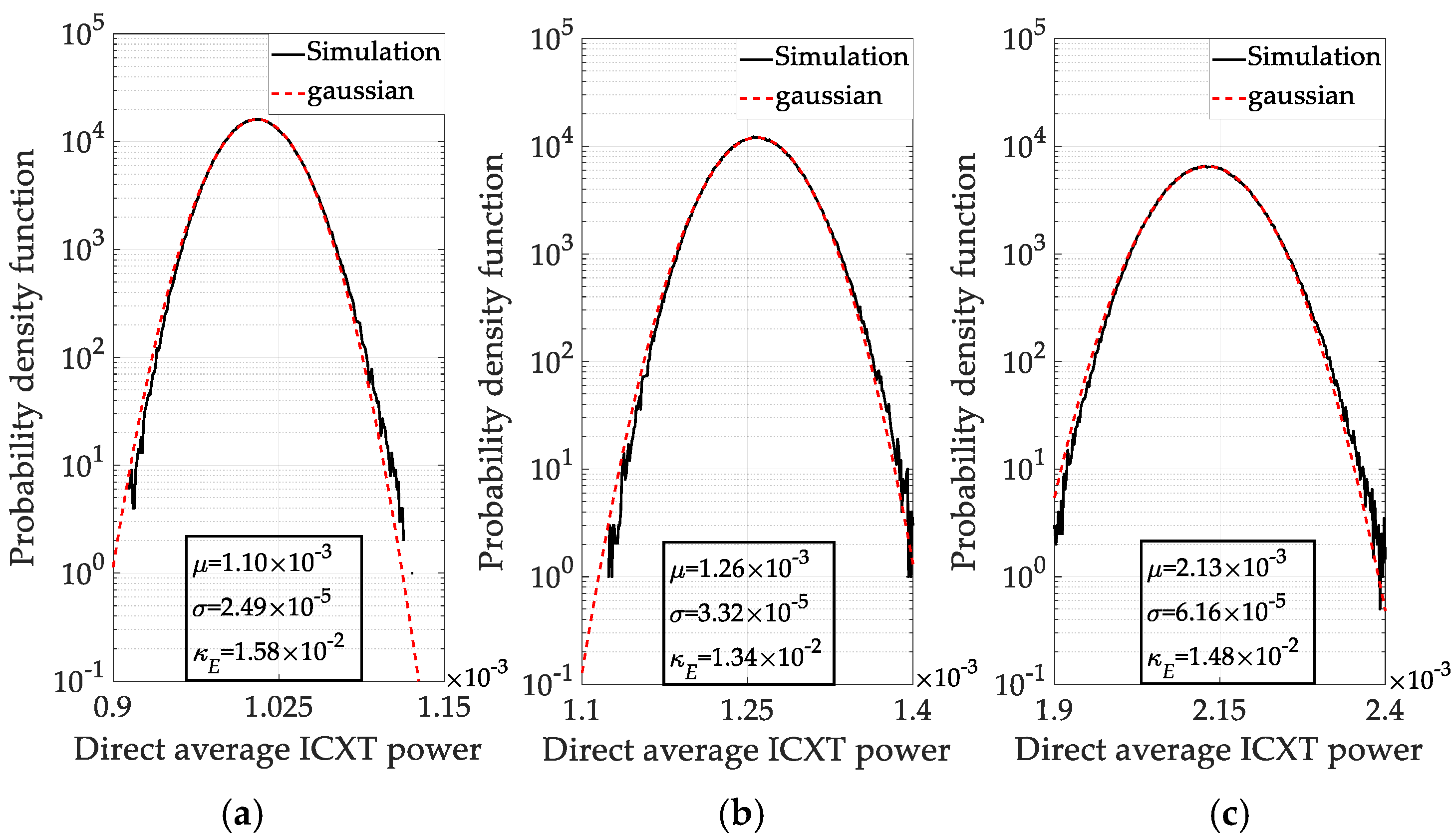
Figure 2 shows the PDFs of the direct average ICXT power obtained with random CDL, considering (a) random segment lengths L_i,k (and constant power coupling coefficient, h_ref, along the MCF link); (b) random power coupling coefficients, h_i,k, with V_h = 3 dB (and constant segment length, L_ref = 2 km); and (c) random power coupling coefficients, h_i,k, with V_h = 6 dB (and constant segment length, L_ref = 2 km). Gaussian PDFs with the same mean and standard deviation as the ones obtained by simulation are also shown in Figure 2. As a Gaussian PDF has null excess kurtosis, the excess kurtosis κ_E is also shown in Figure 2 to quantify how much an estimated PDF is close to the Gaussian shape [20]. As a reference, with random CDL only, i.e., with V_h = 0 and Δ_L= 0, the PDF mean, standard deviation, and excess kurtosis are, respectively, μ = 1.01 × 10⁻³, σ = 2.41 × 10⁻⁵, and κ_E = 1.27 × 10⁻² [15]. Each PDF shown in Figure 2 is obtained with 10⁶ iterations of MC simulation of the long-haul MCF link. In each iteration, one MCF link realization is created with segments that have random characteristics. For that link realization, the direct average ICXT power is obtained at the MCF link output from Equation (8). Considering all MC realizations, a histogram of the direct average ICXT power is built, from which the PDF is calculated, and the corresponding mean, standard deviation, and excess kurtosis are obtained.

Figure 2a shows that the randomness of the segment length does not significantly affect the direct average ICXT power, leading to a similar PDF (mean, standard deviation, and excess kurtosis) as the PDF obtained considering only the CDL randomness. Figure 2b,c show that the power coupling coefficients randomness increases the mean and standard deviation of the direct average ICXT power in comparison with the PDF shown in Figure 2a obtained for a constant coupling coefficient. For V_h = 6 dB, the mean increases by 2.9 dB, and the standard deviation increases by 3.9 dB relative to the mean and standard deviation obtained with constant h_ref = 5 × 10⁻¹⁰ m⁻¹ (V_h = 0 dB) in Figure 2a. The Gaussianity of the PDFs is not particularly affected by the randomness of the power coupling coefficients, as the excess kurtoses shown in Figure 2 are very similar.

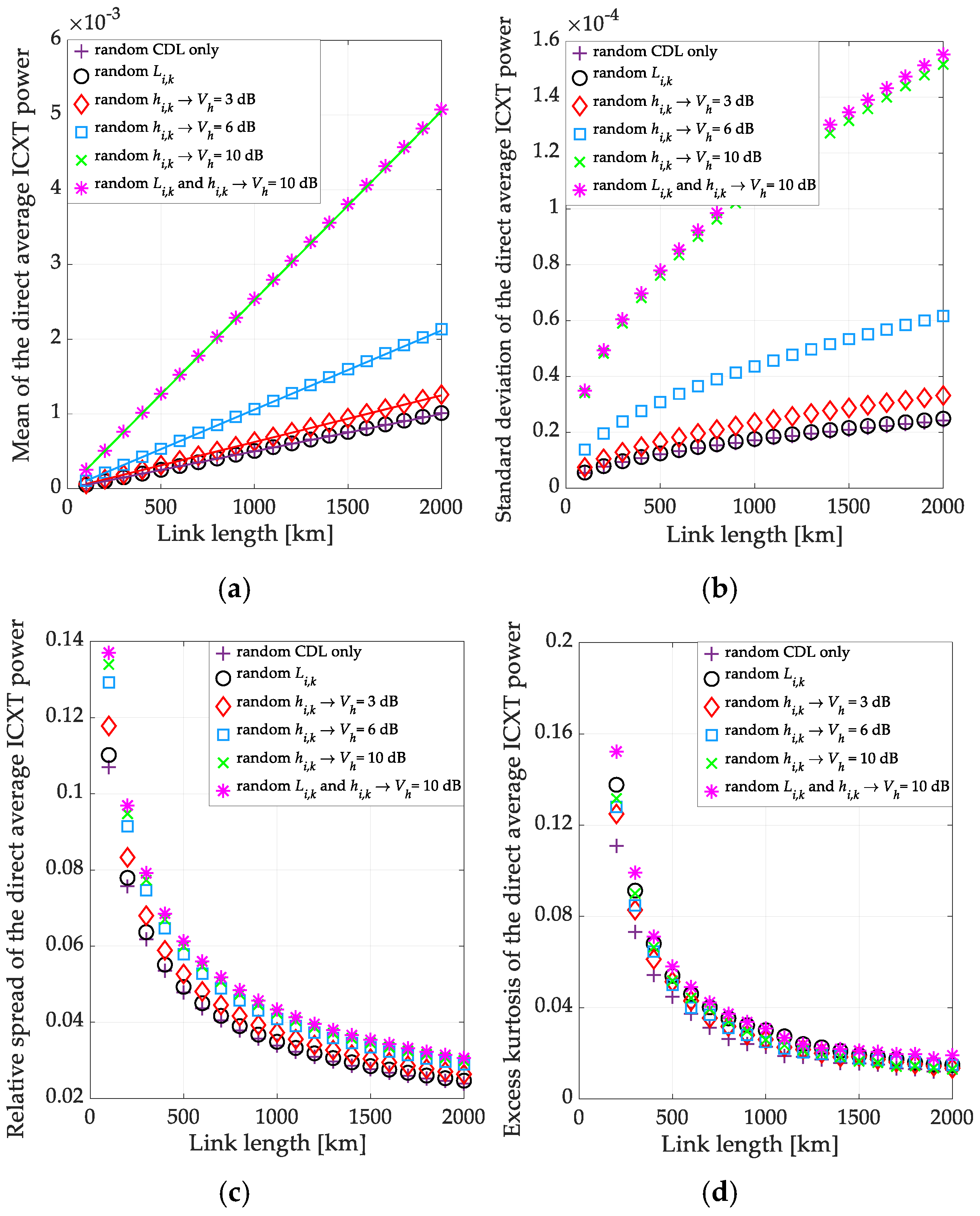
Figure 3a–d show, respectively, the mean μ, standard deviation σ, relative spread σ/μ, and excess kurtosis κ_E of the direct average ICXT power as a function of the link length for different scenarios concerning the randomness of the segment length and the power coupling coefficient. Three scenarios are considered: (i) random L_i,k (with constant h_i,k equal to h_ref); (ii) random h_i,k (with constant L_i,k equal to L_ref) with V_h = 3 dB, 6 dB, and 10 dB; and (iii) random L_i,k and h_i,k with V_h = 10 dB. Random CDL is considered in all scenarios. For each scenario, 10⁷ iterations of MC simulation of the long-haul MCF link are required to obtain stabilized values of the excess kurtosis.

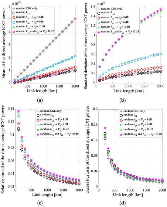
Figure 3a shows that the mean of the direct average ICXT power is practically independent of the randomness of the segment length for the variation between [1.5, 2.5] km considered for L_i,k. This is concluded from the overlapping of the curves corresponding to the mean obtained with random L_i,k (‘ο’symbols) and the mean obtained with random CDL only ( ‘+’ symbols). Hence, it can be concluded from Figure 3a that the mean practically depends only on the power coupling coefficient randomness, growing for higher V_h, since the power coupling between the two cores is enhanced for higher h_i,k. For V_h = 6 dB (‘☐’ symbols), the mean of the direct average ICXT power practically doubles after 2000 km, relative to the case of random CDL only. For V_h = 10 dB, the mean reaches 5 × 10⁻³ (−23 dB) after 2000 km. In Figure 3a, considering the coupling coefficient randomness, and since N_s spans of equal length have been assumed, we have concluded that the mean is approximated well by $\mu =N_s{\mu }_1$, where ${\mu }_1$ stands for the mean of the direct average ICXT power at the output of the first span [15]. At the output of the first span, the mean can be estimated well by ${\mu }_1=[{10}^{V_h[\mathrm{dB}]/10}+{10}^{-V_h[\mathrm{dB}]/10}]\cdot h_{ref}{L}_{s,1}/2$. The solid lines shown in Figure 3a show the results obtained with this analytical approximation for V_h = 0, 3, 6, and 10 dB (violet, red, blue, and green lines, respectively) and are very close to the corresponding numerical results (represented by the symbols with the same corresponding colors). It is important to also notice that in Figure 3a, for V_h = 10 dB, the curves obtained with random L_i,k and h_i,k (symbols ‘∗’) and obtained with random h_i,k (symbols ‘×’) are superimposed.

Figure 3b shows that the standard deviation of the direct average ICXT power grows with the power coupling coefficient randomness since the coupled power increases for higher h_i,k. For V_h = 6 dB, the standard deviation of the direct average ICXT power almost triples after 2000 km, relative to the case of random CDL only. Further inspection of the results revealed that the standard deviation varies with the number of spans $\sigma =N_s^{1/2}{\sigma }_1$, where ${\sigma }_1$ stands for the standard deviation of the direct average ICXT power at the output of the first span. This behavior has also been observed in [15], with only random CDL generation. As for the mean, the impact of the randomness of the segment length is practically negligible on the standard deviation in comparison with the scenario of random CDL only.

Although the power coupling coefficient randomness increases the mean and standard deviation of the direct average ICXT level, Figure 3c,d show that the relative spread and the excess kurtosis are marginally affected by the randomness of h_i,k (and also L_i,k), particularly for long link lengths. The relative spread determines the excess of direct average ICXT power induced by the random effects between segments relative to the case without randomness. The definition of the excess of direct average ICXT power is given by [15] the following equation:

$$\Delta X{T}_{dir}\left[dB\right]=10{\log }_{10}\left(1+k\sigma /\mu \right)$$

(9)

where k sets the range of variation of ΔXT_dir. Considering k = 3 in Equation (9) (corresponding to the 3σ rule of thumb), 99.7% realizations of the long-haul MCF link have direct average ICXT power in the range [μ − 3σ, μ + 3σ], and half of them lead to ΔXT_dir ≥ 0 dB. In Figure 3c, as for shorter link lengths the relative spread is higher, the excess of direct average ICXT power is also higher. For a 100 km link length, ΔXT_dir = 1.496 dB (σ₁/μ₁ = 0.1371), for random h_i,k and V_h = 10 dB, and ΔXT_dir = 1.21 dB (σ₁/μ₁ = 0.1070), for random CDL only. Considering only random h_i,k, for a 100 km link length, there is an increase of only 0.26 dB of excess ICXT power, relative to the case of random CDL only. As the relative spread approaches zero for longer link lengths, the excess of the direct average ICXT power is also reduced with the increase in the link length. For a 2000 km long link, ΔXT_dir = 0.38 dB (σ/μ = 0.0306), for random h_i,k and V_h = 10 dB, and ΔXT_dir = 0.33 dB (σ/μ = 0.0263) for random CDL only. In the results shown in Figure 3c, it can be concluded that the excess of direct average ICXT power, for links with N_s equal length spans, can be estimated well by knowing the relative spread at end of the first span, ${\sigma }_1/{\mu }_1$, even in the presence of coupling coefficient randomness and segment length randomness.

In Figure 3d, with the increase in the link length (a higher number of concatenated segments), the excess kurtosis decreases and approaches zero, meaning that, for longer link lengths, the PDFs of the direct average ICXT power become more Gaussian-distributed [15]. In these cases, the number of MCF segments is sufficiently high to meet the central limit theorem. For shorter link lengths (a lower number of concatenated MCF segments), as the excess kurtosis is farther away from zero, the PDFs are less Gaussian [15]. The Gaussian behavior variation with the link length seems to be tied to the behavior of the relative spread of the direct average ICXT power with the link length. For longer link lengths, lower relative spreads are observed for more Gaussian PDFs. For shorter link lengths, the lower Gaussianity of the PDFs leads to higher relative spread.

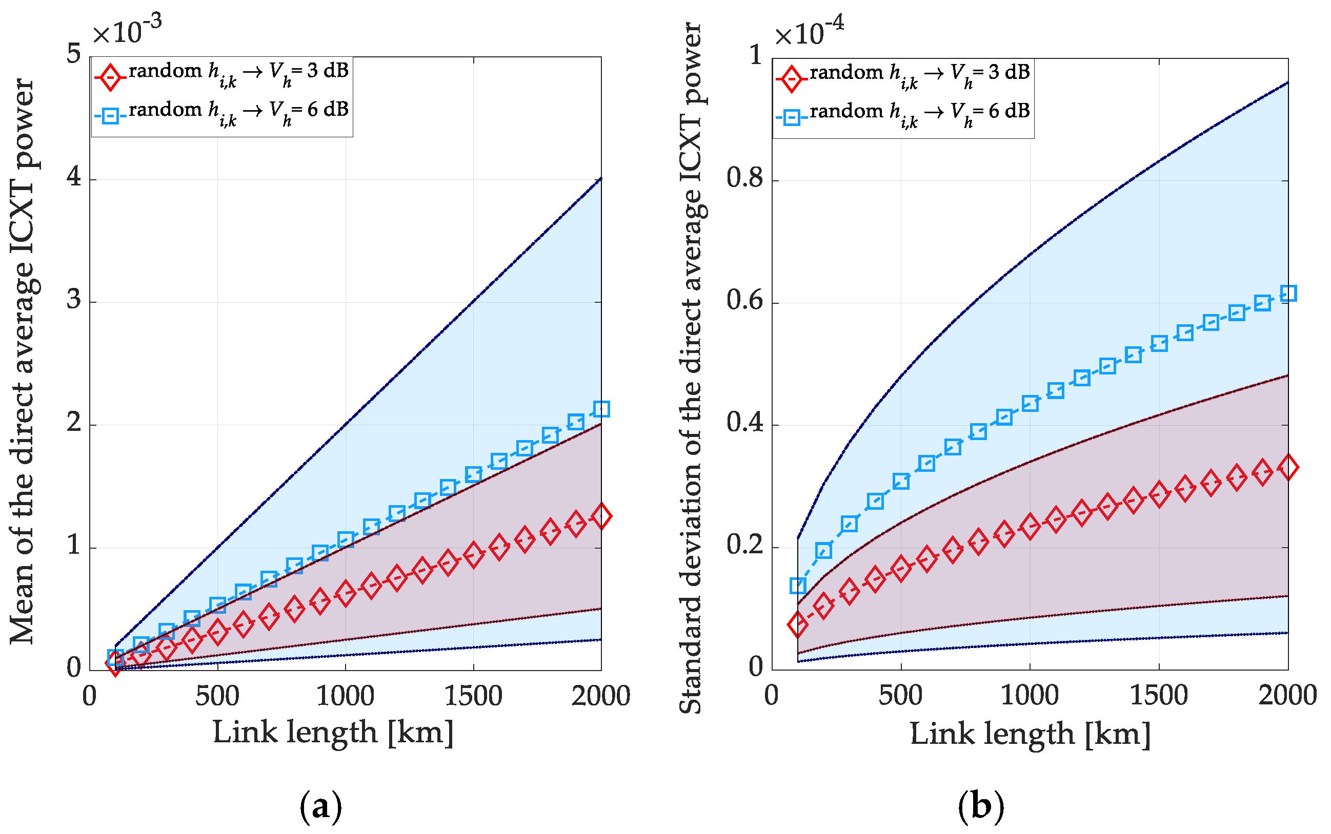
Figure 4a,b show, respectively, the mean and standard deviation of the direct average ICXT power as a function of the link length, considering the randomness of CDL and of the power coupling coefficient with V_h = 3 dB and 6 dB. The shaded areas represent the variation of the mean and standard deviation, considering random CDL, but with constant (deterministic) h_i,k along all MCF segments. The boundaries of the shaded area correspond to the minimum and maximum coupling coefficients of, respectively, h_i,k = 2.5 × 10⁻¹⁰ m⁻¹ and h_i,k = 1 × 10⁻⁹ m⁻¹, for V_h = 3 dB (red area), and to the minimum and maximum coupling coefficients of, respectively, h_i,k = 1.25 × 10⁻¹⁰ m⁻¹ and h_i,k = 2 × 10⁻⁹ m⁻¹ for V_h = 6 dB (blue area).

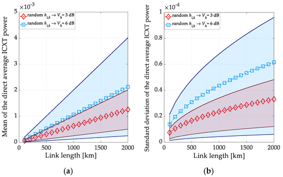
Figure 4 shows that the randomness of the coupling coefficient along the MCF segments leads to a reduction in the mean and standard deviation of the direct average ICXT power (lines with symbols) relative to considering a constant h_i,k with the maximum value (upper bound of the shaded areas). Hence, in Figure 4, it can be concluded that the arbitrariness of the MCF segments concatenation may reduce the power coupling coefficient impact on the direct average ICXT power relative to MCF links with a constant coupling coefficient. This advantage provided by the random concatenation of MCF segments with different characteristics has been also observed in numerical studies when only considering the impact of random CDL on the direct average ICXT power in MCF links [15] and in field experiments with concatenated MCF segments with common characteristics but fabricated by different manufacturers [18].

4. Conclusions

This work assessed the effect of concatenating arbitrary MCF segments with different characteristics on the statistical behavior of the direct average ICXT power in long-haul uncoupled MCF links. The impact of the randomness of segment length, coupling coefficient, and CDL on the PDF, mean, standard deviation, relative spread, and excess kurtosis of the direct average ICXT power was studied.

We concluded that the randomness of the segment length does not significantly affect the direct average ICXT power, leading to a similar PDF (mean, standard deviation, relative spread, and excess kurtosis) as the one obtained while considering only the CDL randomness. The randomness of the power coupling coefficient of the MCF segments can lead to a significant increase in the mean and standard deviation of the direct average ICXT power since more optical power is coupled between cores. For V_h = 6 dB, the mean almost doubles, and the standard deviation almost triples, relative to the case of random CDL only, for 2000 km long links. However, the effect of the coupling coefficient randomness on the relative spread is reduced relative to the case of the constant coupling coefficient (and random CDL). For 100 km long links, it leads to an excess of direct average ICXT power increase of only 0.26 dB. For longer links, this increase is even less significant. The coupling coefficient randomness does not significantly affect the nearly Gaussian distribution PDF observed for a sufficiently high number of concatenated MCF segments.

References

- Beppu, S.; Soma, D. Progress and challenges of coupled core MCF transmission. In Proceedings of the 49th European Conference on Optical Communications (ECOC 2023), Glasgow, UK, 1–5 October 2023. paper Tu.B.2.1. [Google Scholar]
- Downie, J.; Jung, Y.; Makovejs, S.; Edwards, M.; Richardson, D. Cable capacity and cost/bit modeling of submarine MCF systems with MC-EDFA alternatives. J. Lightw. Technol. 2023, 41, 3559–3566. [Google Scholar] [CrossRef]
- Hayashi, T.; Nagashima, T.; Inoue, A.; Sakuma, H.; Suganuma, T.; Hasegawa, T. Uncoupled multi-core fiber design for practical bidirectional optical communications. In Proceedings of the 2022 Optical Fiber Communications Conference and Exhibition (OFC), San Diego, CA, USA, 6–10 March 2022. paper M1E.1. [Google Scholar]
- Matsui, T.; Sagae, Y.; Yamada, Y.; Nakajima, K.; Matsuo Inoue, T.; Katayama, K.; Inada, Y. High figure-of-merit multi-core fiber with standard cladding diameter for long-haul and wide-band transmission. J. Lightw. Technol. 2024, 42, 4124–4131. [Google Scholar] [CrossRef]
- Zhang, L.; Chen, J.; Agrell, E.; Lin, R.; Wosinska, L. Enabling technologies for optical data center networks: Spatial division multiplexing. J. Lightw. Technol. 2020, 38, 18–30. [Google Scholar] [CrossRef]
- Luís, R.; Puttnam, B.; Rademacher, G.; Shinada, S.; Hayashi, T.; Nakanishi, T.; Saito, Y.; Morishima, T.; Furukawa, H. Multicore fiber interconnects for multi-terabit spine-leaf datacenter network topologies. J. Opt. Commun. Netw. 2023, 15, C41–C47. [Google Scholar] [CrossRef]
- Gené, J.; Winzer, P.; Chen, H.; Ryf, R.; Hayashi, T.; Sasaki, T. Towards broadly optimum multi-core fiber designs. In Proceedings of the 45th European Conference on Optical Communication (ECOC 2019), Dublin, Ireland, 22–26 September 2019. [Google Scholar] [CrossRef]
- Kobayashi, Y.; Hayashi, T. Behavior and measurement method of inter-core crosstalk in multicore fibers with core-dependent loss. Opt. Exp. 2023, 31, 502–508. [Google Scholar] [CrossRef] [PubMed]
- Tamura, Y.; Hayashi, T.; Nakanishi, T.; Hasegawa, T. Low-loss uncoupled two-core fiber for power efficient practical submarine transmission. In Proceedings of the Optical Fiber Communication Conference 2019, San Diego, CA, USA, 3–7 March 2019. paper M1E.5. [Google Scholar]
- Soma, D.; Beppu, S.; Wakayama, Y.; Sumita, S.; Takahashi, H.; Yoshikane, N.; Morita, I.; Tsuritani, T.; Suzuki, M. Trans-pacific class transmission over a standard cladding ultralow-loss 4-core fiber. Opt. Exp. 2022, 30, 9482–9493. [Google Scholar] [CrossRef] [PubMed]
- Matsui, T.; Kobayashi, T.; Kawakara, H.; Gabory, E.; Nagashima, T.; Nakanishi, T.; Saitoh, S.; Amma, Y.; Maeda, K.; Arai, S.; et al. 118.5 Tbit/s transmission over 316 km-long multi-core fiber with standard cladding diameter. In Proceedings of the 2017 Opto-Electronics and Communications Conference (OECC) and Photonics Global Conference (PGC), Singapore, 31 July–4 August 2017. [Google Scholar]
- Hayashi, T. Accuracy of analytical expressions for Rayleigh backscattered crosstalk in bidirectional multi-core fiber transmissions. Opt. Exp. 2022, 30, 23943–23952. [Google Scholar] [CrossRef] [PubMed]
- Koshiba, M.; Kokubun, Y.; Nakagawa, M.; Ohzeki, M.; Takenaga, K. Behavior of intercore crosstalk in square-layout uncoupled four-core fibers. IEICE Electron. Exp. 2022, 19, 1–5. [Google Scholar] [CrossRef]
- Cartaxo, A. Loss imbalance effect on inter-core crosstalk in bidirectional uncoupled multi-core fiber transmission. J. Lightw. Technol. 2023, 41, 5911–5921. [Google Scholar] [CrossRef]
- Rebola, J.; Cartaxo, A. Statistical characterization of the effect of random core loss on the intercore crosstalk in long-haul uncoupled multicore fiber links. Opt. Exp. 2024, 32, 26069–26081. [Google Scholar] [CrossRef]
- Oda, T.; Nakamura, A.; Koshikiya, Y. Test method of splice points for constructing uncoupled multi-core fiber transmission line. J. Lightwave Technol. 2024, 42, 1616–1625. [Google Scholar]
- Rebola, J.; Cartaxo, A.; Alves, T. Impact of the combined effect of random core-dependent and splice losses on intercore crosstalk performance in weakly-coupled multicore fibers. In Proceedings of the 2024 24th International Conference on Transparent Optical Networks (ICTON), Bari, Italy, 14–18 July 2024. paper We.B3.3. [Google Scholar]
- Mori, T.; Yamada, Y.; Shibahara, K.; Matsui, T.; Kikuchi, M.; Sagae, Y.; Soma, D.; Beppu, S.; Nagashima, T.; Morishima, T.; et al. Applicability of Standard Cladding Diameter Multi-Core Fiber Cables for Terrestrial Field. J. Lightw. Technol. 2024, 42, 1044–1055. [Google Scholar] [CrossRef]
- Zitelli, M.; Matera, F.; Settembre, M.; Tamburrini, M. Dispersion-managed link with randomly variable map length. In Proceedings of the Conference on Lasers and Electro-Optics (CLEO 2000), San Francisco, CA, USA, 7–12 May 2000. paper CMF4. [Google Scholar]
- Mood, A.; Graybill, F.; Boes, D. Introduction to the Theory of Statistics; McGraw-Hill: New York, NY, USA, 1974; Chapter 2. [Google Scholar]
Disclaimer/Publisher’s Note: The statements, opinions and data contained in all publications are solely those of the individual author(s) and contributor(s) and not of MDPI and/or the editor(s). MDPI and/or the editor(s) disclaim responsibility for any injury to people or property resulting from any ideas, methods, instructions or products referred to in the content. |
© 2024 by the authors. Licensee MDPI, Basel, Switzerland. This article is an open access article distributed under the terms and conditions of the Creative Commons Attribution (CC BY) license (https://creativecommons.org/licenses/by/4.0/).