Study of Optical Rogue Waves in Two-Dimensional Disordered Lattices

Abstract

We probed the impact of both the degree of disorder and nonlinearity on rogue waves (RWs) in two-dimensional disordered lattices. Our results unveiled that an increase in the disorder level under linear conditions heightened the probability of RW occurrence and simultaneously contracted the “long tail”. Interestingly, with the introduction of nonlinearity, this “long tail” became shorter compared with linear conditions. Nevertheless, in the context of disordered media, RW occurrence probability demonstrated relative stability—a distinct deviation from its conduct within homogeneous media.

1. Introduction

Initially introduced by Draper in 1965 [1], rogue waves (RWs) have since garnered ongoing research interest. RWs are generated through several mechanisms. Current linear theoretical studies suggest that RWs primarily result from either spatial or spatio-temporal self-focusing, which is caused by the varying group speeds of different wave components. These phenomena often occur in dispersive or diffractive media [2,3]. Researchers in the field of nonlinearity suggest that RWs are significantly affected by nonlinearity, which is primarily due to the nonlinear overlay of waves. This process is facilitated by modulation instability (MI) [4,5], i.e., a plane wave with a small perturbation can evolve into RWs. They can also result from the collision of high-amplitude and breathing solitons [6]. In addition, granularity and inhomogeneity are also factors affecting the generation of rogue waves in nonlinear systems [7]. RWs have been observed in diverse fields, from oceanography [8] to Bose–Einstein condensation [9,10], atmospheric sciences [11], plasma physics [12], nonlinear optics [13,14], and even finance [15]. The study of RWs in optical systems began with the 2007 discovery of high-amplitude pulses in fiber-optic supercontinuum spectra by Solli [16], akin to oceanic RWs. Subsequent research quickly explored the nonlinear characteristics of RWs in optics, including their production in fiber-optic supercontinuum spectra [17,18,19] and generation through soliton collisions [20,21,22]. The majority of prior studies have primarily concentrated on temporal RWs, paying significantly less attention to spatial RWs. Recently, research on spatial RWs has been increasing. Chen et al. [23] found that under appropriate nonlinear conditions, the nonlinear evolution of wide Gaussian light conforms to the RWs’ probability distribution in saturated nonlinear media. RWs have also been observed in disordered one-dimensional (1D) photonic lattices [24]. This reveals the interesting occurrence of Anderson localization, which is a phenomenon resulting from interference caused by repeated electron scattering in a randomly defective potential [25]. This leads to a transformation of the eigenmodes from extended (Bloch waves) to localized [26]. Similarly, Schwartz et al. [27] inspected the nonlinear impact on Anderson localization experimentally. In reference [28], it was found that localization in disordered systems limits the discrete diffraction of light, constraining light waves transversely. Rivas et al. [24] explored how the disorder level could affect RW generation probability under linear conditions with a narrow beam. It was observed that RWs vanished when the disorder level was extremely high due to the strong local effect. Lee et al. [29] suggested that broad beams in a disordered system might undergo a filamentation phenomenon triggered by the localization effect. This may be akin to the MI effect in a homogeneous medium. However, under nonlinear conditions, the experiments and statistical results of intensity events in a two-dimensional disordered lattice with a wide beam are still unclear. Comparing these results with those in homogeneous media could be intriguing.

In this paper, we analyze the behavior of RWs in two-dimensional disordered lattices numerically and experimentally. A disordered environment was established in a saturated nonlinear medium. A wide Gaussian beam (GB) was used to excite RWs, and the statistical patterns of RWs were investigated and compared with the statistics of RWs in a homogeneous medium. For numerical simulations, we utilized the nonlinear Schrödinger equation [30] to describe the evolution and propagation of light in the nonlinear medium.

2. Experiment

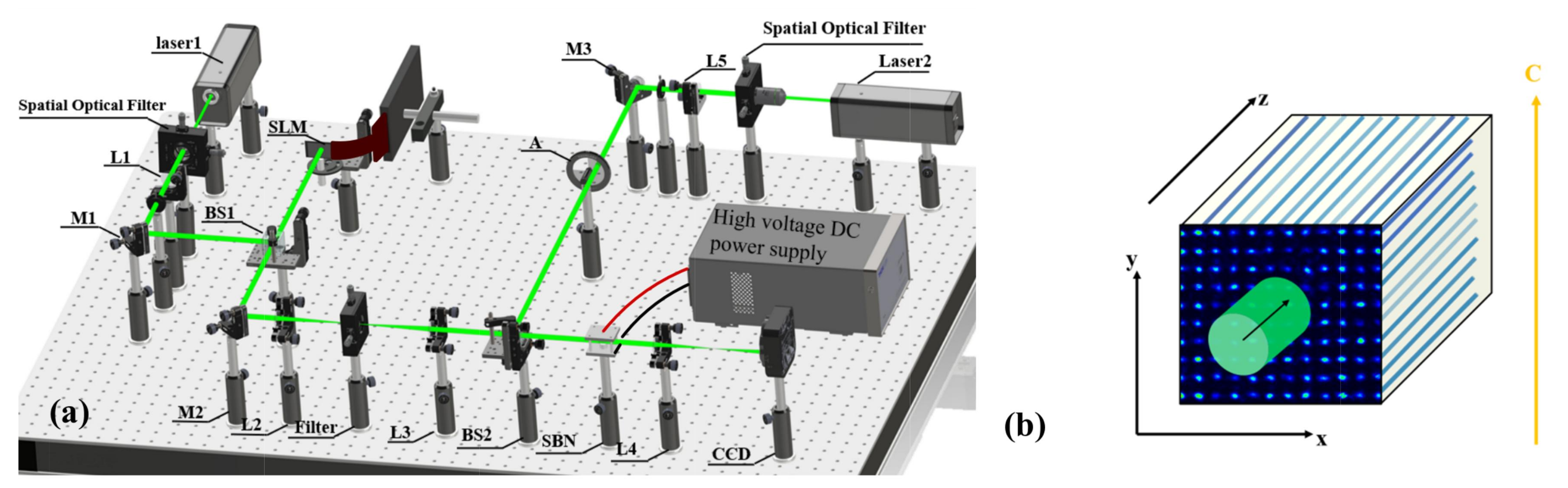
Our experimental setup, depicted in Figure 1, employed two 532 nm wavelength CW lasers. An ordinary polarized writing beam from Laser 1 was expanded into an approximately planar wave by a “Spatial Optical Filter” and L1. Then, the writing beam modulated by a spatial light modulator (SLM) [HOLOEYE PLUTO-2] carried the desired disordered pattern information and incidence into a 0.002% ${\mathrm{CeO}}_2$-doped SBN:61 photorefractive crystal with an applied bias voltage. Due to the saturated nonlinear effect, the writing beam generated two-dimensional disordered lattices in the crystal, which corresponded to the optical field distribution. 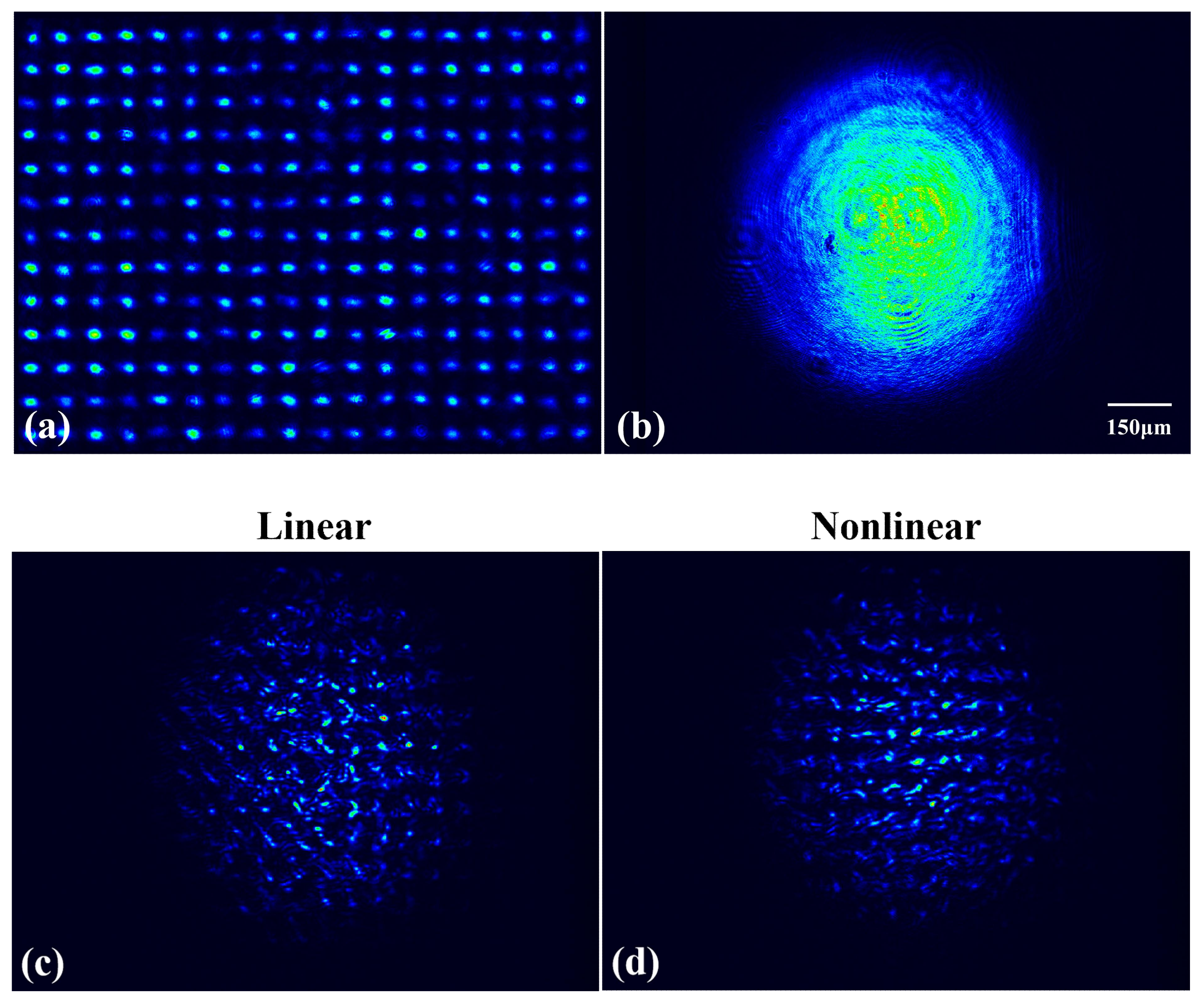Figure 2a shows typical two-dimensional disordered lattices. The lattices were periodic lattices relative to distance but with an inhomogeneous intensity distribution. The input power of the writing beam was 120 $\mathsf{\mu }$W. The SBN crystal had a 5 × 5 ${\mathrm{mm}}^2$ cross-sectional area and was 10 mm in length along the propagation coordinate z. Another extraordinary polarized light beam as the probe beam was also launched into the crystal. The probe beam from Laser 2 was expanded to a wide Gaussian beam (GB) by the “Spatial Optical Filter” and L5, and a pinhole was used to filter out the harmonic components of the Gaussian light, retaining only the 0th-order light. Figure 2b shows the probe beam, approximately 450 $\mathsf{\mu }$m in width at half maximum and around 0.5 $\mathsf{\mu }$W in input power. The saturation nonlinearity was controlled through the applied bias voltage along the optical axis of the crystal. The distribution of the output light was recorded by a CCD camera.

In the experiment, the level of disorder was proportional to light-induced refractive index modulation. In the photorefractive SBN crystal, the refractive index modulation ($\Delta n$) is described by the equation below:

$$\Delta n=\frac{1}{2}{n}_o^3{\gamma }_{13}\frac{U}{d}\frac{{\psi }_w\left(x,y,z\right)}{1+{\left|{\psi }_w\left(x,y,z\right)\right|}^2}$$

(1)

where the refractive index for ordinary polarized light ($n_o$) is 2.31, the electro-optical coefficient (${\gamma }_{13}$) is 45 pm/V, U is the applied bias voltage, d is the height of crystal, and ${\psi }_w\left(x,y,z\right)$ corresponds to the slowly varying light wave envelope of the writing beam. So, $\Delta n$ can be controlled by U when we maintain constant input power for the writing beam and vary its disorder level by the applied voltage.

In a photorefractive SBN crystal, the interaction between light and matter requires time to respond. During the experiment, the probe beam was initially blocked, and the writing beam needed about ten seconds to establish disordered lattices and reach a stable state. Then, the probe beam was turned on to propagate along the z-axis in disordered lattices. Linear output patterns were recorded at the instant of probe beam incidence due to the slow nonlinear response. We recorded nonlinear output patterns when the probe beam reached nonlinear propagation, five seconds later. Linear and nonlinear output patterns were recorded at different disorder levels. Figure 2c,d provide illustrations of the light field distribution under linear and nonlinear states at U = 800 V, respectively. For each set voltage level (600 V, 800 V, and 1000 V), we conducted 30 repeat experiments in different modulation distributions of the same disorder level, each yielding an analysis based on approximately 4000 waves.

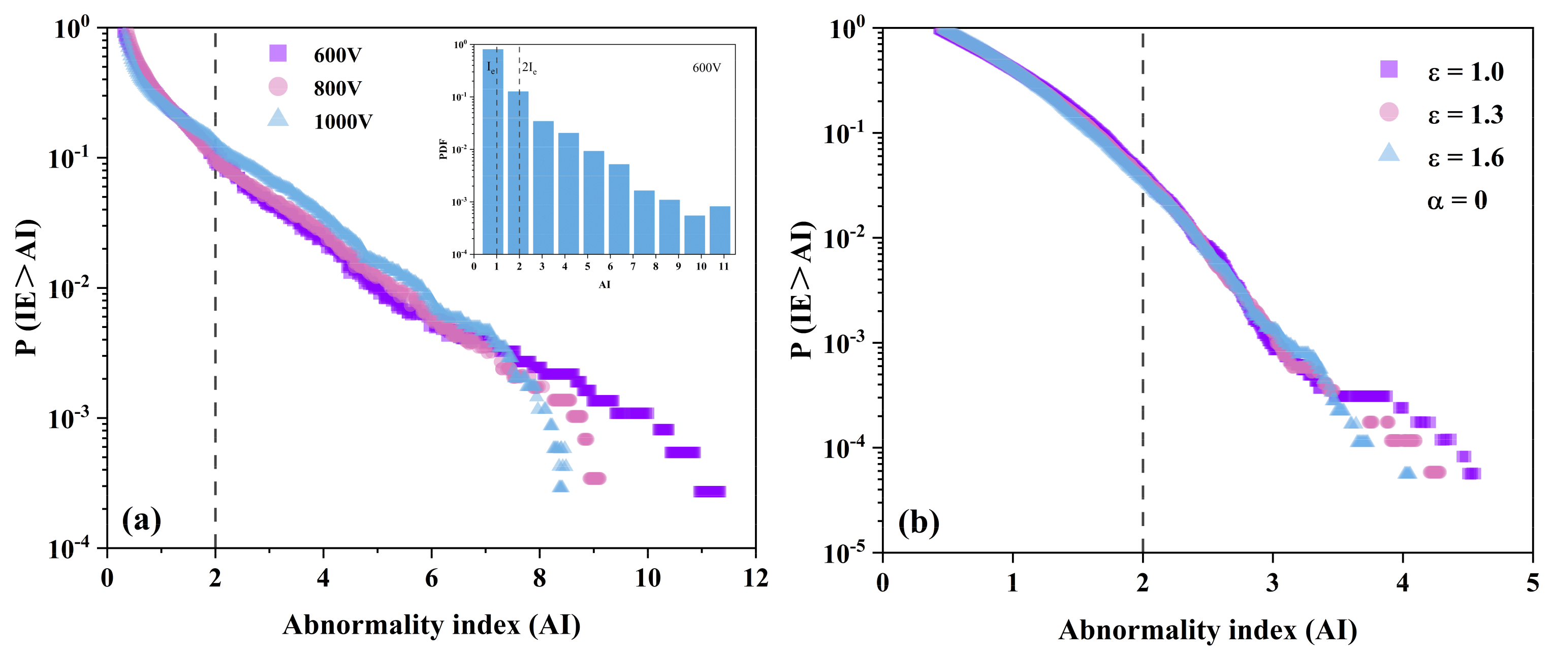
By following a standard criterion on RWs [31], we consider RWs those with intensities larger than twice a significant $I_{\mathrm{e}}$, which is defined as the average value of the highest-intensity tertile of the corresponding probability density function (PDF) distribution. PDF is a function used to describe the probability of a continuous random variable’s output being near a certain value. I is denoted as the intensity of every wave packet. Waves with an abnormality index $AI\equiv I/I_{\mathrm{e}}>2$ (marked with a gray dashed line) were considered RWs. For example, the PDF corresponding to $AI$ = 3 represents the probability of the wave’s intensity being around three times $I_e$ [inset in Figure 3a]. To determine the probability of RW occurrence, we computed P(IE > AI) = 1 − cumulative PDF. This represents the probability of having an intensity event (IE) with an AI larger than a certain value, P(IE > AI) [Figure 3a,b]. Hence, the probability of having RWs corresponds to the value at which the data cross AI = 2.

Following this, we conducted a probability analysis of all waves for output contours at different disorder levels. These levels corresponded to voltage settings of 600 V, 800 V, and 1000 V, all of which were tested under linear conditions, as depicted in Figure 3a. To our surprise, we found evidence of RWs even under linear states. Interestingly, as the disorder level increased, the statistical distribution of P(IE > AI) displayed a shorter “long tail”. We suggest that as the disorder level increases, discrepancies in the mode between distinct refractive index channels become more substantial, and the mutual coupling starts to deteriorate. This, in turn, attenuates the interaction between the propagating probe beams within the channels, consequently making the generation of high-energy RWs more challenging. By using various voltage levels to represent different disorder levels, we calculated RW occurrence probability under linear conditions, with $P_{\mathrm{L}}$ (600 V) = 9.7%, $P_{\mathrm{L}}$ (800 V) = 10.2%, and $P_{\mathrm{L}}$ (1000 V) = 13.1% [Figure 3]. As the disorder level increased, the probability of RW occurrence also increased.

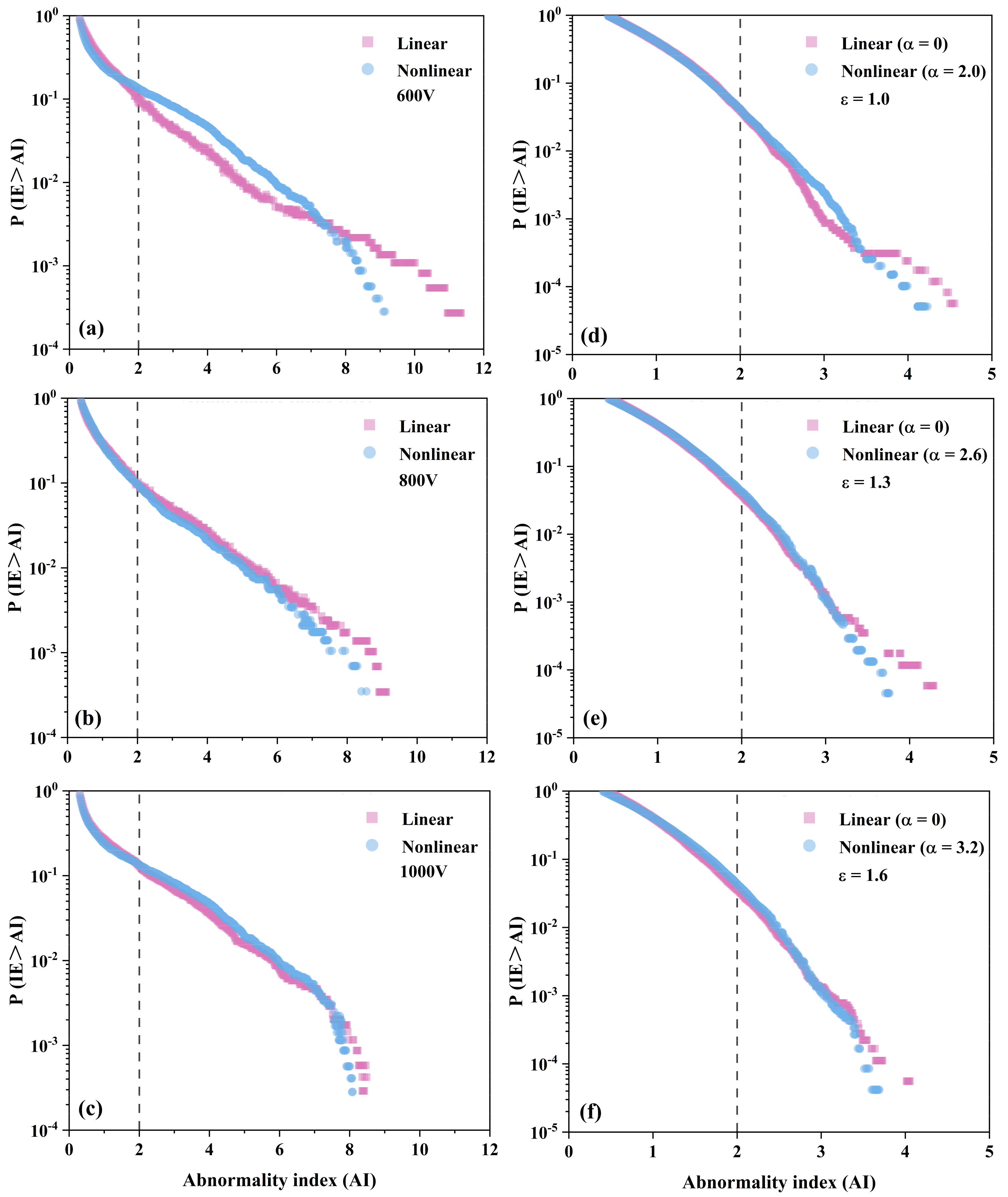
Figure 4a–c illustrate a comparative P(IE > AI) at the same disorder level, for both linear and nonlinear conditions. Interestingly, when nonlinearity is introduced under the same disordered conditions that are applied to the linear conditions, the “long tail” becomes noticeably shorter. Then, the RW occurrence probability under nonlinear conditions was calculated, with $P_{\mathrm{NL}}$ (600 V) = 10.6% [Figure 4a], $P_{\mathrm{NL}}$ (800 V) = 10.9% [Figure 4b], and $P_{\mathrm{NL}}$ (1000 V) = 13.4% [Figure 4c]. The introduction of nonlinearity accentuated the wave differences, increasing the probability of RW occurrence and noticeably shortening the “long tail”.

Further, we found that the red line (linear) in Figure 4 sometimes appeared above and sometimes below the blue line (nonlinear). We suggest that the inclusion of nonlinearity indeed leads to the further focusing of the probe light wave guided by the disordered lattices, particularly for waves with lower energy. This focusing effect results in a decrease in the probability of wave generation with a lower abnormality index (AI), an increase in the probability of rogue wave occurrence (AI > 2), and a concurrent decrease in the probability of extremely high-energy wave occurrence. Consequently, the blue line (nonlinear) exhibits an overall side “S”-shaped trend, with a low-to-high-to-low pattern, explaining the instances where the red line (linear) crosses above or below the blue line (nonlinear) in Figure 4. Furthermore, as the level of disorder increases, the dominant role of nonlinearity diminishes, and the disorder gradually takes over as the primary determinant. This transition is reflected in the increasingly similar trends between the red line (linear) and the blue line (nonlinear), as is evident in Figure 4a–c.

3. Numerical Simulation

To verify the experimental results, we numerically simulated the phenomena. The propagation of a probe beam in the SBN crystal was approximated by a nonlinear Schrödinger equation (NLSE) with saturable nonlinearity in the form [30]

$$i\frac{\partial \psi (x,y,z)}{\partial z}+\beta {\nabla }_{\perp }^2\psi (x,y,z)+\left(\frac{\alpha }{1+{\left|\psi (x,y,z)\right|}^2}+\Delta \xi \right)\psi (x,y,z)=0$$

(2)

where $\psi \left(x,y,z\right)$ corresponds to the slowly varying light wave envelope, z to the propagation coordinate, $\beta$ to the diffraction coefficient, and ${\nabla }_{\perp }^2$ to the transverse Laplace operator. The nonlinear coefficient is denoted by $\alpha$, and it is proportional to the external applied voltage in the experiment. $\Delta \xi$ correlates with disordered refractive index modulation, corresponding to $\Delta n$ in the experiment. By utilizing a random number generator, we configured disordered refractive index modulation with the depth of $\Delta \xi$ set as $\epsilon$, and the range of $\Delta \xi$ was [0, $\epsilon$]. In the experiment, the level of disorder and the intensity of nonlinearity were simultaneously controlled by an applied voltage, with linear and nonlinear conditions being distinguished merely by the evolution time of the probe beam. To make the simulation as close as possible to the experiment, we used parameter $\alpha$ to control the intensity of nonlinearity, while the depth ($\epsilon$) reflected the level of disorder. $\epsilon$ = 1.0, $\epsilon$ = 1.3, and $\epsilon$ = 1.6 corresponded to the disorder levels in the experiment at the voltage of 600 V, 800 V, and 1000 V, respectively. When $\alpha$ = 0, it corresponded to the linear conditions in the experiment. $\alpha$ = 2, $\alpha$ = 2.6, and $\alpha$ = 3.2 corresponded to the nonlinear conditions under 600 V, 800 V, and 1000 V in the experiment, respectively. Furthermore, we conducted simulations 1000 times for different random distributions of $\Delta \xi$ with equal $\epsilon$, resulting in an analysis of approximately 32,000 waves per $\Delta \xi$. P(IE > AI) was performed at varying modulation depths when $\alpha$ = 0, as shown in Figure 3b.

The RW occurrence probability was then calculated, with $P_{\alpha = 0}$ ($\epsilon$ = 1.0) = 3.64%, $P_{\alpha = 0}$ ($\epsilon$ = 1.3) = 3.86%, and $P_{\alpha = 0}$ ($\epsilon$ = 1.6) = 4.05% [Figure 3b]. For $\alpha$ = 0, there is a slight increase in the probability of RW occurrence in correlation with an increased level of disorder. Figure 4d–f illustrate P(IE > AI) at the same disorder depth values ($\epsilon$) but for varying nonlinear intensities ($\alpha$). It is worth noting that as the nonlinearity increases, the generation of high-energy RWs becomes less likely, an observation that aligns with the experimental outcomes. We calculated the RW occurrence probability at different disorder levels and nonlinear intensities, with $P_{\alpha = 2}$ ($\epsilon$ = 1.0) = 4.17% [Figure 4d], $P_{\alpha = 2.6}$ ($\epsilon$ = 1.3) = 4.30% [Figure 4e], and $P_{\alpha = 3.2}$ ($\epsilon$ = 1.6) = 4.41% [Figure 4f]. When $\alpha \ne 0$, the probability of RW generation increases slightly at the same value of $\epsilon$ compared with $\alpha$ = 0. The general trend of these numerical results is consistent with the experiments. The discrepancy between the experimental and simulation values may be due to the approximations made in the simulation.

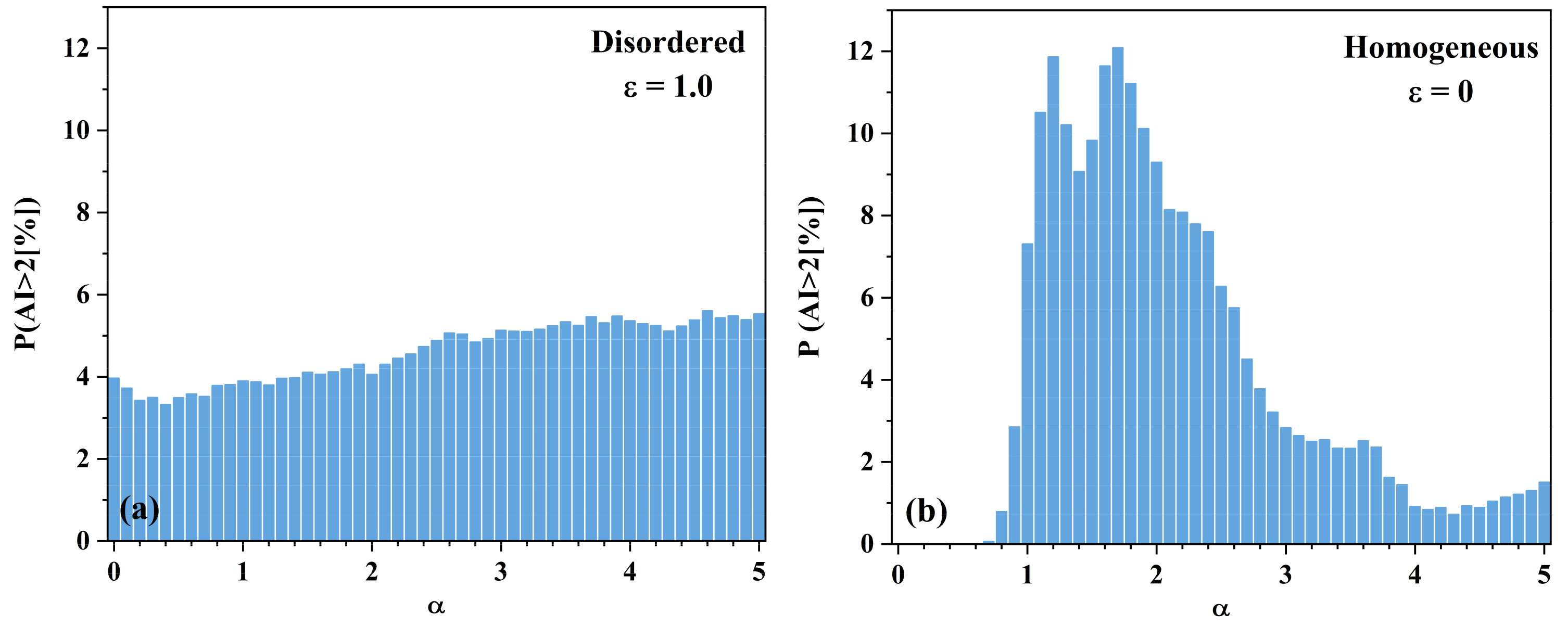
To analyze the transformation of RWs in a homogeneous medium ($\Delta \xi$ = 0), we kept the same parameters of the probe beam used in the disorderly medium. A noise seed, averaging zero and peaking at 20% of the GB amplitude at a specific position, was included. The nonlinear intensity was gradually increased from 0 to 5 at increments of 0.01. For the disordered medium, we set $\epsilon$ = 1.0. Subsequently, we determined the statistics of RW occurrence probability for the outgoing surface under varying nonlinear intensities. For enhanced visibility, we broke down the nonlinear intensity interval for these statistics into 0.1 per segment. We then contrasted the probability trend of RW occurrence with the nonlinear intensity ($\alpha$) in both disordered and homogeneous media. The resultant probability distribution of the RWs is visualized in Figure 5.

Our results reveal a markedly higher RW occurrence probability in the homogeneous medium, 12.1%, compared with a considerably lower value, 5.61%, for the disordered medium. It is worth pointing out that the presence of RWs in a disordered medium is independent of nonlinearity. Rather, the disorder level in the system is the primary determinant of RW occurrence probability, whereas nonlinearity plays a substantially marginal role. On the other hand, in a homogeneous medium, RW formation incorporates a discernible influence of a nonlinear strength threshold of 0.7. Interestingly, a moderate increase in nonlinear intensity initially prompts an increase in the probability of RW occurrence, attributable to MI. As nonlinearity becomes more potent, the role of MI grows increasingly dominant, triggering a significant surge in RWs. However, when nonlinearity achieves an excessively high level, an equilibrium between the effects of MI and diffraction is established. Consequently, RW occurrence probability experiences a dip, subsequently stabilizing in a range between 1% and 3%. Therefore, our study underscores a distinct difference in RW generation probability between disordered and homogeneous media.

4. Conclusions

This study delves into the intricate statistical law of RWs in two-dimensional disordered lattices. The intriguing findings reveal a corresponding increase in the probability of RW occurrence as disorder levels increase under linear conditions, consequently tightening the statistical tail of RWs. However, with the introduction of nonlinearity, the statistical tail undergoes further contraction, but the probability of RW occurrence retains relative stability. Anderson localization significantly reduces the interactions among filaments. Unlike in a homogeneous medium, where the probability of RW occurrence varies significantly with nonlinear changes, this phenomenon is suppressed here. Instead, it maintains a relatively stable trend with a slightly upward tendency. This compelling observation starkly contrasts with the dynamics in homogeneous media. It indirectly reflects that the interaction between adjacent waves in the disordered system is weak, which provides a train of thought for future study on the nonlinear interaction between adjacent Anderson local waves.