Article

The Impact of Pulse Shaping on Coherent Dynamics near a Conical Intersection

Department of Physics, School of Physical Science and Technology, Ningbo University, Ningbo 315211, China
*
Authors to whom correspondence should be addressed.
Photonics 2024, 11(6), 511; https://doi.org/10.3390/photonics11060511
Submission received: 6 April 2024 / Revised: 20 May 2024 / Accepted: 20 May 2024 / Published: 27 May 2024
(This article belongs to the Special Issue Ultrafast Optics and Applications)

Abstract

:
Utilizing lasers to probe microscopic physical processes is a crucial tool in contemporary physics research, where the influence of laser properties on excitation processes is a focal point for scientists. In this study, we investigated the impact of laser pulses on the quantum yield of electronic wave packets near conical intersections (CIs). To do so, we employed the time non-local quantum master equation to calculate the time-evolution dynamics of wave packets on excited-state potential energy surfaces (PESs) and projected them onto effective reaction coordinates. The waveform of laser pulses was manipulated by varying the relative amplitude, pulse duration, and center wavelengths of Gaussian profiles. Our calculations revealed that the shape of laser pulses has a discernible impact on the dynamic evolution of electrons in excited states. Furthermore, our research indicated that different pulse profiles exhibit a maximum variation of 6.88% in the quantum yields of electronic wave packets near CIs. Our calculations demonstrate the influence of laser pulse waveform on excitation processes, providing a feasible method for exploring the coherent control of wave packets at conical intersections characterized by strong nonadiabatic coupling.

1. Introduction

Laser pulses serve as crucial tools to investigate microscopic physical processes. The laser excitation can induce a transition of the electronic wave packet from the molecular ground to one or multiple excited states. The degeneracy of potential energy surfaces (PESs) in the configuration space of polyatomic molecules induces strong nonadiabatic coupling between two PESs. The resulted CI mixes the quantum dynamics of the electrons and the nuclei, implying that the Born–Oppenheimer approximation breaks down [1,2,3,4]. The degeneracy of the molecular PESs permits an ultrafast radiationless transition of the wave packet from upper electronic excited states to the lower ones, whereby the conical intersection structure opens a nonadiabatic energy channel, significantly accelerating the efficiency of energy transfer [5]. Due to the strong vibronic coupling, the wave packet dynamics in the vicinity of a CI can be monitored by its associated vibrational coherence of the reaction coordinates by using the coherent spectroscopic techniques [6,7]. Pump–probe spectroscopy, with configurations, is a powerful tool to monitor the dynamics of a wave packet passing through the CI. For instance, to study the ultrafast photoisomerization of rhodopsin, Polli et al. employed transient absorption spectroscopy to unravel the timescales of ultrafast isomerization [8]. They revealed the detailed timescale of photoisomerization by monitoring the frequency shift of the stimulated emission from excited state to ground state. Moreover, in the transient absorption spectrum, the vibrational coherence has been examined both in the reactant and product states to investigate the wave packet dynamics in the vicinity of the CI [9,10]. An evidence of the CI in the isomerization [11,12] and singlet fission [13,14] was also provided by tracking the coherent transfer of a wave packet along the intra- and intermolecular vibrational coordinates. More recently, Miller et al. and coworkers employed two-dimensional electronic spectroscopy to reveal the nonadiabatic dynamics in rhodopsin [11]. With this, they were able to detect the enhancement of electronic transitions from ground to the excited state between two PESs when the wave packet approached the degenerate point. Femtosecond-stimulated Raman spectroscopy (FSRS) is another valuable tool to detect the time evolution of the vibrational coherence. The FSRS has been used to study the isomerization process in rhodopsin [15] and it was estimated to occur within 200 fs or less. The recently developed FSRS re-examined the isomerization process, and its timescale has been measured to be shorter than 50 fs [16]. In Mukamel’s work, PE-stimulated Raman gain/loss (PE-SRG/L) and coherent anti-Stokes Raman scattering (PE-CARS) due to monochromatic excitation and PE femtosecond-stimulated Raman spectroscopy (PE-FSRS) are considered. It was discovered that the dependence on the plasmon resonance, picosecond and femtosecond pulse characteristics, and molecular vibrational properties are evident in the density matrix-derived PE-FSRS intensity expression [17]. The photoisomerization of stilbene has also been investigated and the structural changes have been revealed by the gradual shift of the torsional mode [18]. Moreover, the two-dimensional FSRS has been recently constructed and applied to study the anharmonicity of the vibrational coherence of charge-transfer modes of an artificial dimer system [19,20,21]. In addition, the ultrafast electron pulses have been employed to study the isomerization process, and the gradual changes in structures has been shown when a wave packet passes through the CI [22].
The essential physical process of radiationless transitions in the CI can be well captured by a two-state two-mode model [23,24,25]. It has been proposed to study the photoisomerization dynamics in rhodopsin [24]. To monitor the nonadiabatic dynamics, the motion of the wave packet on the PESs has been projected onto the effective reaction coordinates, and the dissipation of the electronic wave packet has been treated by quantum master equations [26,27,28]. The two-state two-mode model has been further simplified by Duan et al. by applying a unitary transformation of the effective reaction coordinates into the harmonic bath and by solving the resulting non-Markovian dynamics using the hierarchy equation of motion to achieve numerically exact results [29]. Moreover, the lifetime of tuning and coupling modes has been modulated to investigate their impact on quantum efficiency in a CI system with strong nonadiabatic coupling [30]. Through this, we observed that the quantum yield of the motion of wave packet can be modulated up to 20%. To capture the signature of the CI, attosecond Raman spectroscopy has been theoretically proposed to detect the transient electronic coherence of wave packets in the vicinity of the CI [31,32]. Furthermore, time-resolved electron or X-ray diffraction has also been proposed to catch the signature of the CI by directly monitoring the motion of the molecular structure [33,34,35,36]. Although the nonadabatic dynamics in the CI has been extensively studied by experimental and theoretical calculations, the detailed dynamics and the key factors impacting the quantum efficiency of the system are still elusive.
The feasibility of pulse modulation has also achieved rapid development in recent years. Valentyn I. Prokhorenko and Andrea M. Nagy modulated the phases and amplitudes of the spectral components in the photoexcitation pulse, showing that the absolute quantity of 13-cis retinal formed upon excitation can be enhanced or suppressed by ±20% of the yield observed using a short transform-limited pulse with the same actinic energy [37]. Xinhua Xie and Katharina Doblhoff-Dier, in their work, control various fragmentation reactions of a series of polyatomic molecules (e.g., acetylene, ethylene, 1,3-butadiene) via the optical waveform of intense few-cycle laser pulses. Their study both experimentally and theoretically shows that the mechanism responsible for this control is the inelastic ionization from inner-valence molecular orbitals by repeatedly colliding electron wave packets, whose recollision energy in few-cycle ionizing laser pulses strongly depends on the optical waveform [38]. Liat Levin and Wojciech Skomorowski used an ab initio model to show that control is achieved by purification combined with chirp-dependent Raman transitions. An experimental closed-loop-phase optimization using a learning algorithm yielded an improved pulse that utilizes vibrational coherent dynamics in addition to chirp-dependent Raman transitions. The results show that the coherent control of binary photoreactions is feasible even under thermal conditions [39]. Furthermore, the pulse chirp can represent a convenient parameter to tune the beam temporal profile from an experimental point-of-view. By applying ultrashort chirped pulses, it can be found that the timescale of excitation is comparable to that of the electronic dephasing while the following adiabatic process relies on the chirp of the pulse inverting the population on a timescale much shorter than the dephasing time [40,41,42].
In this paper, we study the impact of different laser pulses on the quantum efficiency of electronic wave packets near the CI. For this, we monitor the quantum dissipative dynamics and project it on the effective reaction coordinates. We first numerically select the laser pulses and employ them to prepare the electronically excited state after photoexcitation. We track the motion of wave packets on the PESs in the vicinity of the CI. This allows us to unravel the detailed mechanism and discover the key factors, thereby determining the quantum efficiency. Based on our calculations, we observed an obvious impact of the laser profile on quantum efficiency. The maximum optimization can be reached to 6.9% of enhancement with the optimal pulse profile. Our work demonstrates the laser profile do provide an effective tool to enhance the efficiency of quantum yield in a CI system with strong nonadiabatic coupling.

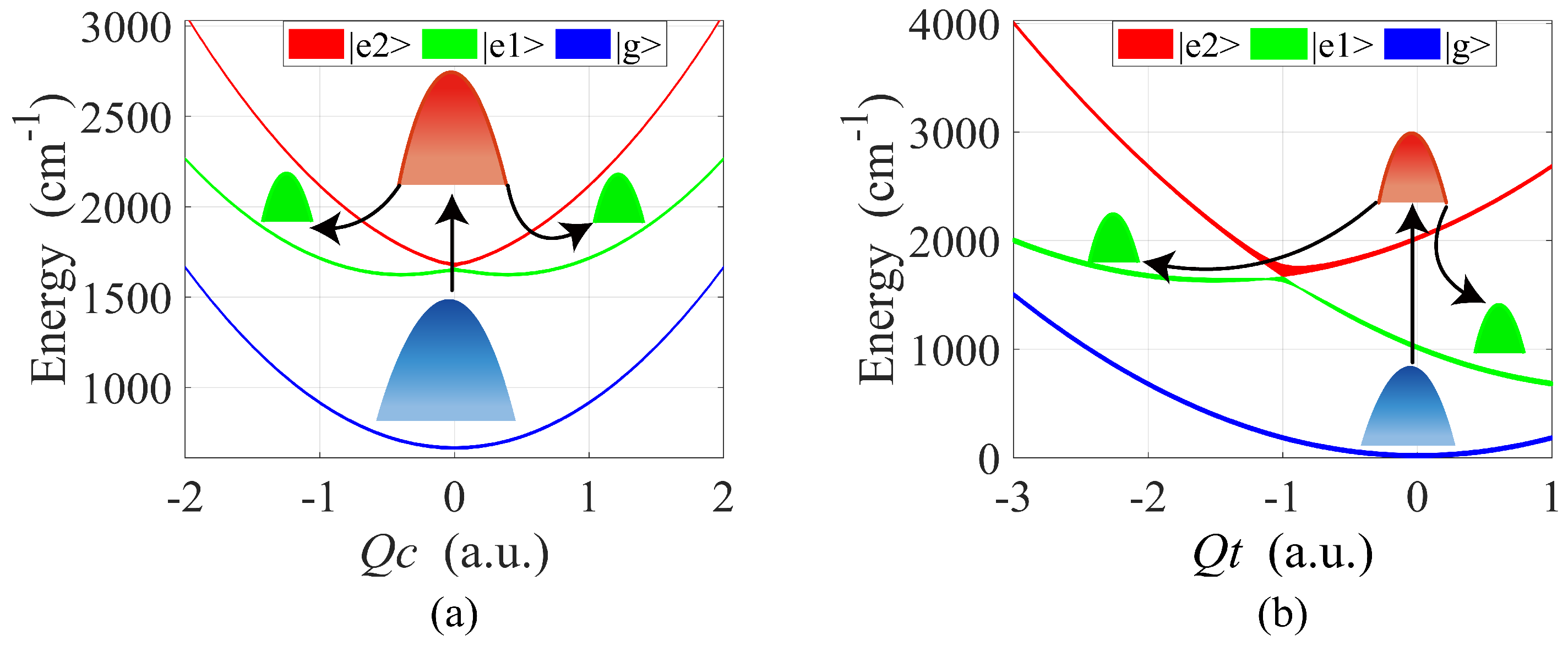
2. Theoretical Model

We start from the three electronic states, | g , | e 1 and | e 2 . We assume two electronic excited states, | e 1 and | e 2 , linearly coupled to two vibrational modes, tuning and coupling modes, respectively. The vibronic coupling is determined by parameter κ . We also assume that the molecular system is coupled to two dissipative baths consisting of an infinite number of harmonic oscillators. Thus, the total Hamiltonian can be written as H = H m o l + H e n v . The system Hamiltonian H m o l = H g + H e 1 + H e 2 , which has the following form:
H g = | g h g g | , H e 1 = | e 1 ( h 1 + ϵ 1 ) e 1 | , H e 2 = | e 2 ( h 2 + ϵ 2 ) e 2 | + ( | e 1 V e 2 | + h . c . ) ,
where h 1 and h 2 are the vibrational Hamiltonian associated with the electronic states | e 1 and | e 2 . h g is the vibrational Hamiltonian of electronic ground state. ϵ 1 , ϵ 2 and V are the energy of electronically excited states and the couplings between the two electronic states, respectively. The two vibrational modes can be written as
h g = 1 2 j = t , c Ω j ( P j 2 + Q j 2 ) , h 1 = 1 2 j = t , c Ω j ( P j 2 + Q j 2 ) κ Q t , h 2 = 1 2 j = t , c Ω j ( P j 2 + Q j 2 ) + κ Q t ;
here, Ω j and P j are the frequency and momentum of the respective vibrational modes; Q j = t , c denotes the coordinate of the mode with frequency Ω j = t , c . For simplicity, we assume that the electronic coupling between the two electronic states is linearly related to Q c , i.e., V = Λ Q c , where Λ is the electronic coupling strength. The bath has been assumed to consist of an infinite number of harmonic oscillators, each linearly coupled to the coupling and tuning modes, respectively. The environmental Hamiltonian is given as
H e n v = i 1 2 p i 2 m i + m i ω i 2 x i + c i Q c m i ω i 2 2 + q i 2 M i + M i ν i 2 y i + t i Q t M i ν i 2 2 .
Here, p i and q i represent the dimensionless momentum and coordinate operators for P i and Q i , respectively. c i and t i , x i and y i , m i and M i , as well as ω i and ν i denote the coupling constants, coordinates, masses, and frequencies for the two modes, respectively. The thermal bath can be described by the spectral density [43], i.e.,
J ( ω ) = 1 2 i c i 2 m i ω i δ ( ω ω i ) , J ( ω ) = 1 2 i t i 2 M i ν i δ ( ω ν i ) .
For the coupling mode and tuning mode, the vibrational modes of the thermal bath follow an Ohmic spectral distribution given by J ( ω ) = η j ω exp ( ω / ω c ) , where η j (j = c, t) represents the vibrational damping strength for each mode and ω c is the cutoff frequency. In addition, we assume that the model is initially located at ground state | g with the lowest vibrational energy level. Thus, the initial density matrix is given by ρ ( 0 ) = | g , 0 t , 0 c .
The light–matter interaction is expressed as μ · E ( t ) , where μ = m = 1 N μ m ( a m + a m ) is the transition dipole moment operator. a m and a m are the creation and annihilation operators, respectively, for the m-th electronic state. The effective electric field of the laser pulse can be represented as E ( t ) = m = 1 N A n E n ( t τ n ) cos ( ω n t k n · r ) , where E n ( t τ n ) represents the waveform of the laser pulse and k n is the wave vector of the pulse. We set the waveform as a Gaussian pulse defined by its full width at half maximum (FWHM), and its form is
E n ( t τ n ) = exp ( 4 · ln 2 · ( t τ n ) 2 / τ p 2 ) ,
where, τ n , τ p and ω n are the central time, pulse duration and the frequency of the laser pulse, respectively.
The laser pulse act on the model at time t = τ n fs and the wave packet can be projected onto the relevant vibrational coordinates in adiabatic representation, which allows us to track the detailed motion of wave packet in the vicinity of the CI with a strong nonadiabatic interaction. The projection process can be written as
P k a d ( Q c , t ) = d Q t Q c | Q t | e k | ρ ( t ) | e k | Q t | Q c , P k a d ( Q t , t ) = d Q c Q c | Q t | e k | ρ ( t ) | e k | Q t | Q c ,
where P k a d represents the probability density for each vibrational mode and e k represents the electronic wave function in the adiabatic representation. The representation from adiabatic to diabatic form can be expressed as | e k = k = e 1 , e 2 S ( Q c , Q t ) k k | e k . Here, S ( Q c , Q t ) k k represents the transformation matrix and | e k is the electronic wave function in the adiabatic representation. In this study, we simulated the process of laser interaction with the model using a phase-matching approach [44,45] and modeled the dynamics of the electronic wave packet near the conical intersection using the time non-local quantum master equation (TNL) method [46,47].
Through derivation and arrangement, the specific form of the main equation used in this article can be written as follows (See Appendix A.1 for detailed deduction):
ρ ( t ) ˙ = L S e f f ρ ( t ) + 0 t d t K ( t , t ) ρ ( t ) + Γ ( t ) , L S e f f = L S + t r B L I ρ B e q + L r e n , K ( t , t ) = t r B L I ( T e t t d t ( 1 P ) L ) ( 1 P ) ( L B + L I ) ρ B e q , Γ ( t ) = t r B L I ( T e t t d t ( 1 P ) L ) ( 1 P ) W ( 0 ) .
In the formula, L S e f f ρ ( t ) , K ( t , t ) and Γ ( t ) represent reversible terms, memory terms and non-homogeneous terms, respectively. The total Hamiltonian of the system H = H S + H B + H I + H r e n , where H r e n is the renormalization term. Correspondingly, the Liouville super operators L S , L I and L r e n , respectively, correspond to the corresponding Hamiltonian operator. In addition, Γ represents a temporal operator, and L S e f f · = i [ H S + H r e n , · ] . ρ e q represents the thermal equilibrium state.
We then set the energy gap between ground and first excited states as ϵ 1 = 1000 cm−1 and the gap between first and second excited states as ϵ 2 = 1000 cm−1. Moreover, the vibrational frequencies of tuning and coupling modes are Ω t = 330 and Ω c = 500 cm−1, respectively. The strength of vibronic coupling κ = 500 cm−1 and electronic coupling strength Λ = 200 cm−1. In order to obtain a converged result, we select the vibrational levels of tuning and coupling modes as 10 and 7, respectively. The temperature is 300 K. Based on these parameters, we plot the PESs along tuning and coupling modes and show them in Figure 1. The quantum yield can be measured by the ratio of the wave packet on the reactant and product states after it reaches the equilibrium. The quantum yield is defined as Y = A A + B , which quantifies the efficiency of photo-induced isomerization from the initial state to the final state.

3. Results

Based on the modeling and parameters, we calculate the population dynamics of the wave packet on the excited electronic states. We firstly prepare the initial wave packet with a Gaussian pulse. The Gaussian line shape of the laser pulse is represented by Equation (8).
In this study, the amplitude of the laser pulse is set to 1000 cm−1 (For detailed description, see Appendix A.2). The model converges within a time of 500 fs. The central time τ n and pulse duration τ p are set to 15 fs and 10 fs, respectively, while the frequency of the pulse is set to 2000 cm−1. We then calculate the population dynamics by time non-local quantum master equation and project the time-resolved wave packet on the reaction coordinates. We show the calculated results in Figure 2a–d.
In Figure 2a and Figure 2b, we show the wave packet dynamics of upper electronic excited states | e 2 along reaction coordinates Q c and Q t , respectively. Moreover, we plot the population dynamics of the wave packet of electronic state | e 1 along Q c and Q t in Figure 2c and Figure 2d, respectively. In this way, we observe that, at initial time, the wave packet is mainly located at the upper electronic excited state. With time propagation, we observe the wave packet moving along the PES and approach the degenerate point, which is shown at −1 along the tuning mode Q t . It is marked as a light blue line in (b) and (d). Moreover, it shows the wave packet passing through the CI and reach the lower excited state at T = 30 fs. More interestingly, it also shows a clear evidence of motion of the wave packet along the reaction coordinate, which reveals the vibrational coherence of the tuning mode. The population dynamics reach the equilibrium after T > 500 fs. With this, we demonstrate that the projection process allows us to clarify the detailed mechanism of wave packet motion. Moreover, the quantum efficiency of the system can be directly monitored by the ratio of wave packet in reactant and product states at equilibrium after a long propagation time.

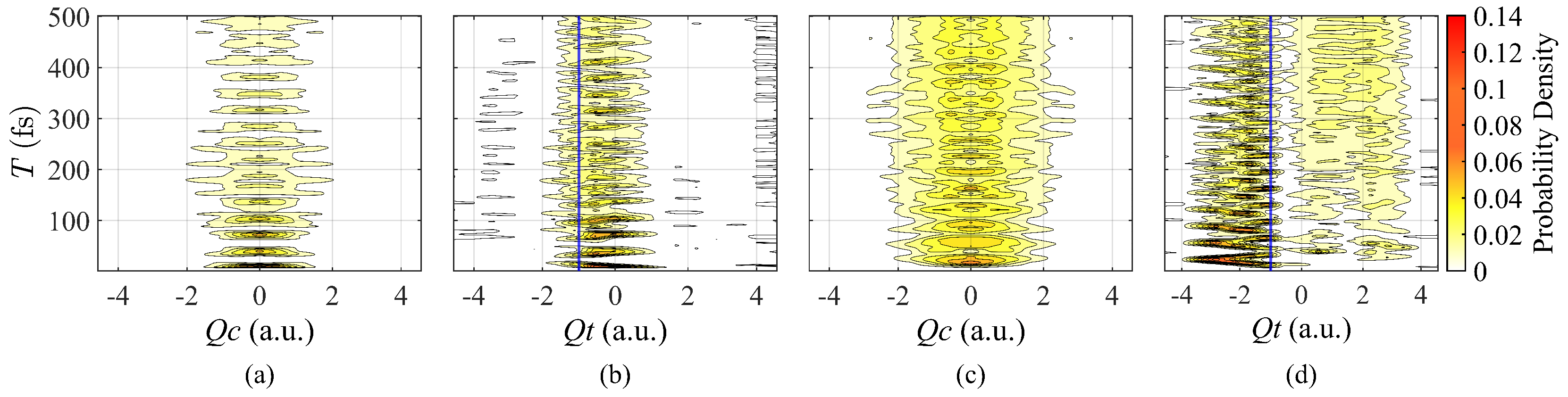
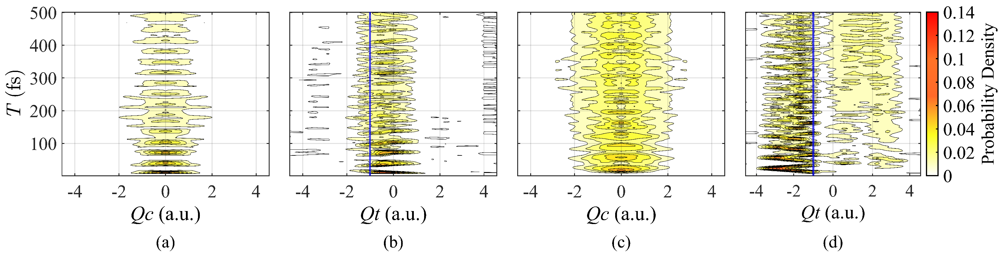
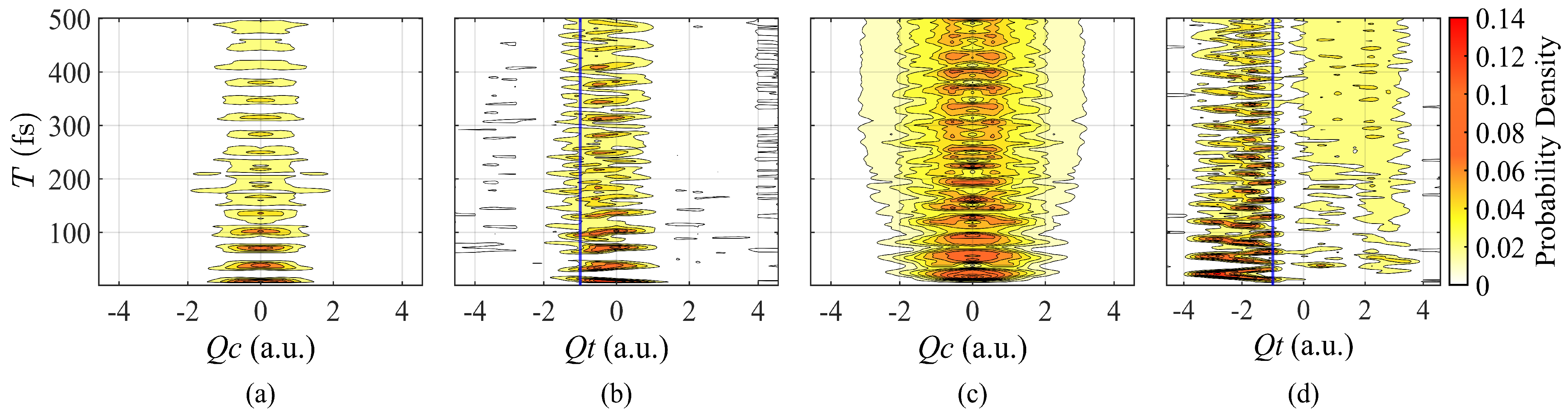
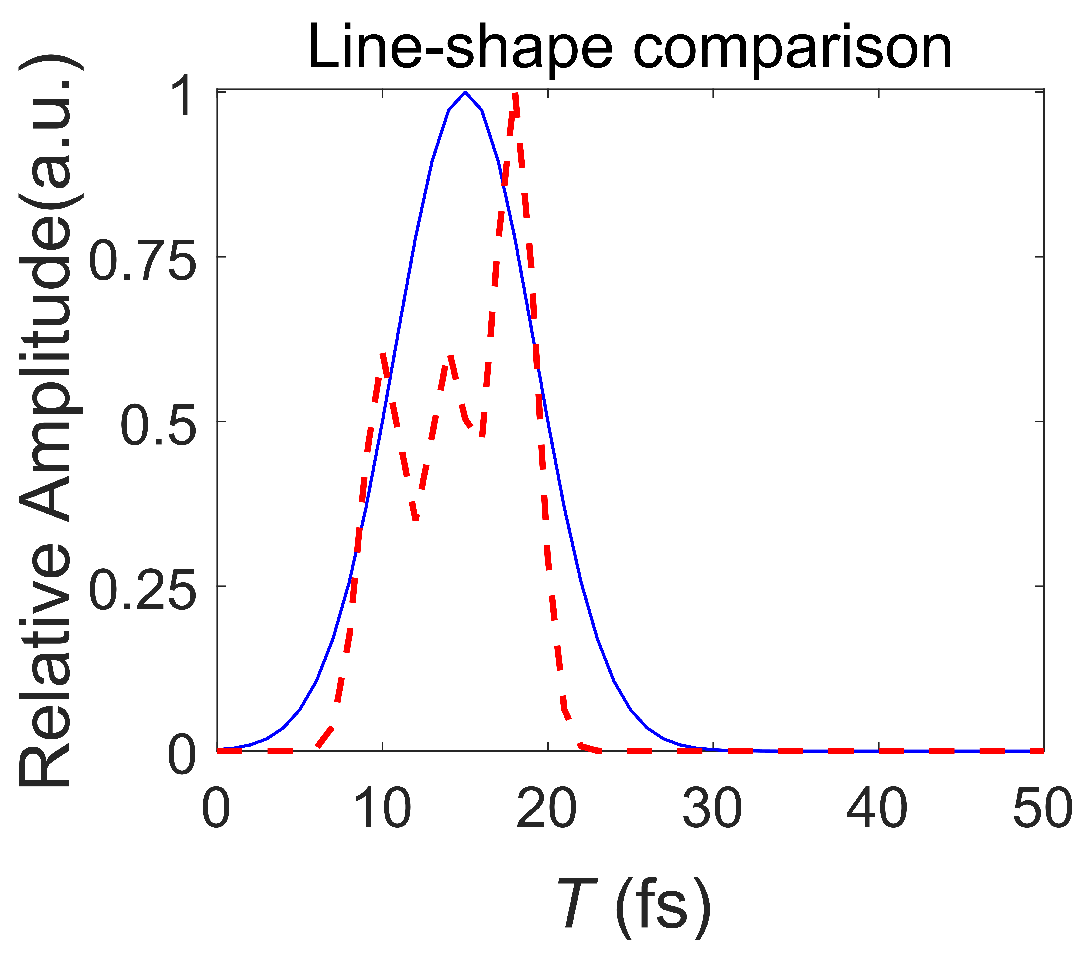
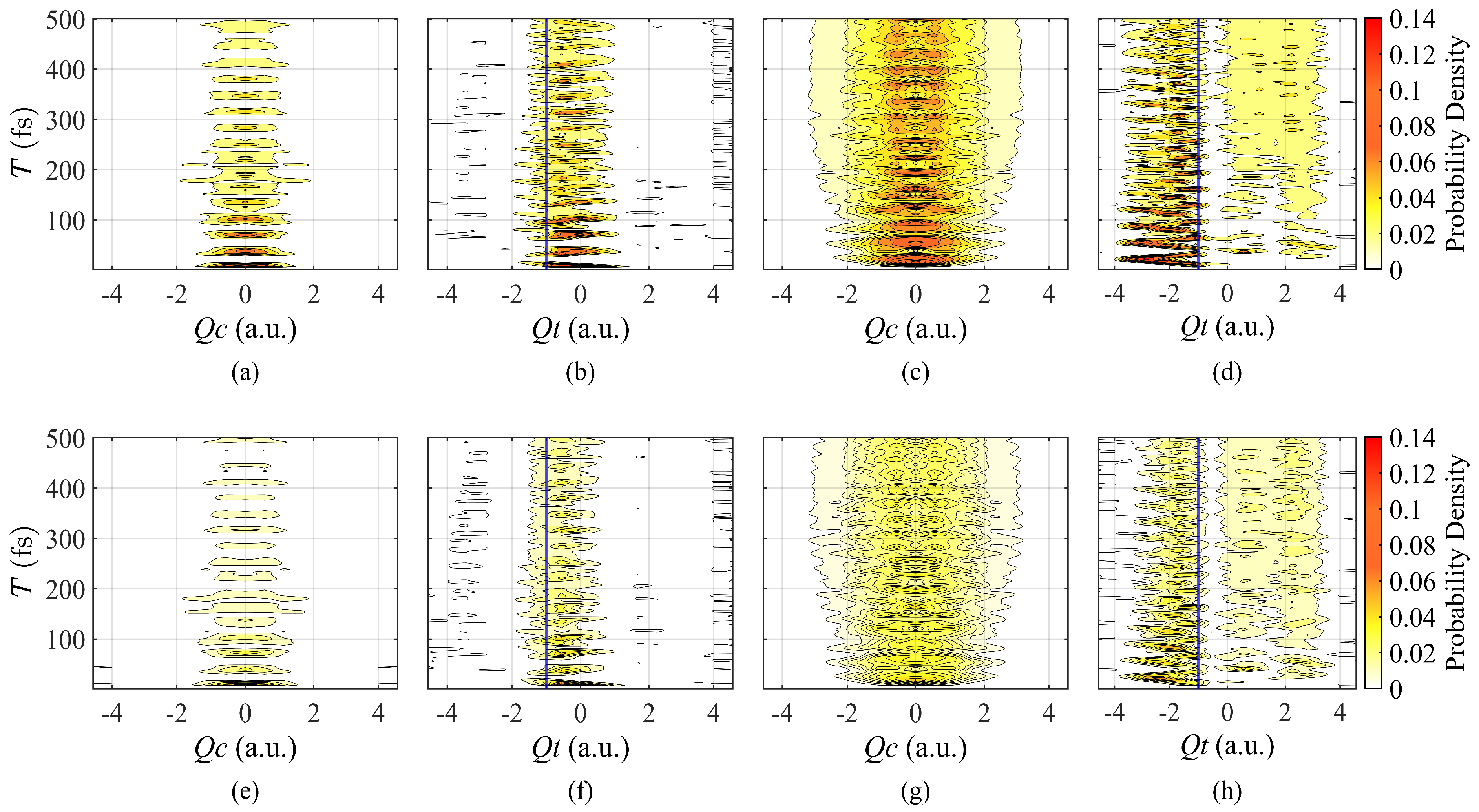
3.1. Synthesis of Artificial Pulse with Modulation of Amplitudes

Next, we study the impact of pulse profile on the quantum efficiency of the CI system. For this, we firstly synthesize the pulse profile by a combination of three pulses. By varying the relative amplitudes and relative positions of three Gaussian pulses, we formed different shapes of ultrashort laser pulses. We modulate the waveform according to the order in which the relative amplitudes appear over time, with the specific form as follows:
E n ( t τ n ) = A i = 1 3 R i exp ( 4 · ln 2 · ( t τ n ) 2 / τ p 2 ) .
Here, the amplitude of the laser pulse is set to 1000 cm−1, identical to the amplitude (A) of each individual Gaussian pulse. The relative amplitudes of the three individual Gaussian pulses are set to 1, 0.6 and 0.2, arranged according to pulse duration. Considering that the difference in average power of laser pulses cannot be too large (as this would lead to kinetic differences caused by pulse energy), combinations of pulse sequences were chosen where the sum of the squares of relative amplitudes exceeds 1. Furthermore, to ensure that the duration of the composite laser pulse matches that of the individual Gaussian pulses, the pulse duration of each sub-line shape is set to 3 fs. Taking 1−0.6−1 as an example, the waveform of the pulse is shown in Figure 3.
We observed that the excitation of the system by laser pulses of different waveforms has a certain impact on the system’s quantum yield. The results indicate that under our settings, there is a difference in quantum yield ranging from 1% to 7%. We selected the waveform setting (0.6−0.6−1) with a more significant difference in quantum yield for further investigation. The corresponding wave packet dynamics for this waveform are plotted in Figure 4. Comparing it with the single Gaussian pulse (Figure 4), we found that the excitation efficiency of the system after laser action is much higher with the single Gaussian waveform laser pulse compared to the composite Gaussian waveform laser pulse, with significant differences in the population intensity on the excited state of the wave packet.
Through the Q c pathway (Figure 4a,c,e,g), in our investigation, we observed a significant attenuation in the stimulated effects of the system upon altering the pulse waveform, attributed to the overall reduced energy of the pulses obtained from the composite Gaussian waveform. Analyzing the coupling mode, we found no significant variation in the period or trend of the wave packet motion on the second excited state before convergence, albeit with a weaker distribution intensity. Similar observations were made on the first excited state, indicating that the amplitude modulation corresponding to this pulse waveform had no significant impact on the system’s dynamical evolution under the coupling mode. However, examining the tuning mode revealed that the scenario with composite Gaussian pulse waveform was stably distributed on both sides of the conical crossing structure in less than 100 fs, and after convergence, the wave packet exhibited a more uniform distribution on the first excited state in the electronic energy levels. This enhancement in quantum yield was quantified, showing an increase of 5.63% in the quantum yield ( Q Y ), reaching 85.2%, compared to the scenario with a single Gaussian pulse waveform. This highlights the impact of the amplitude modulation corresponding to this pulse waveform on the system’s dynamical evolution, particularly in the distribution pattern at lower energy levels under the tuning mode. We computed a series of laser pulses with amplitude modulation and their corresponding differences in quantum yield compared to the single Gaussian waveform pulse, as shown in Figure 5 and Table 1. Another dimension in the table illustrates the issue of "pulse with different durations".

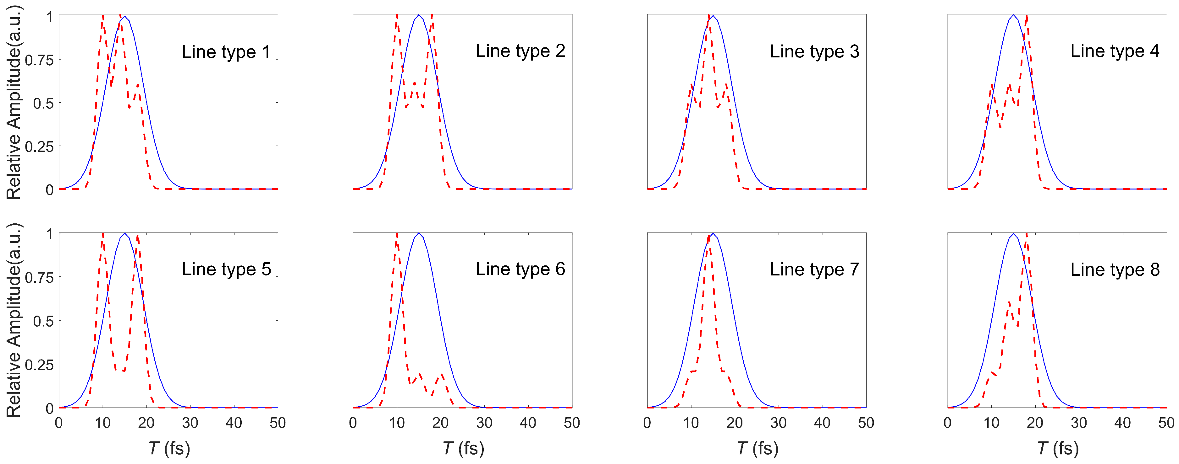
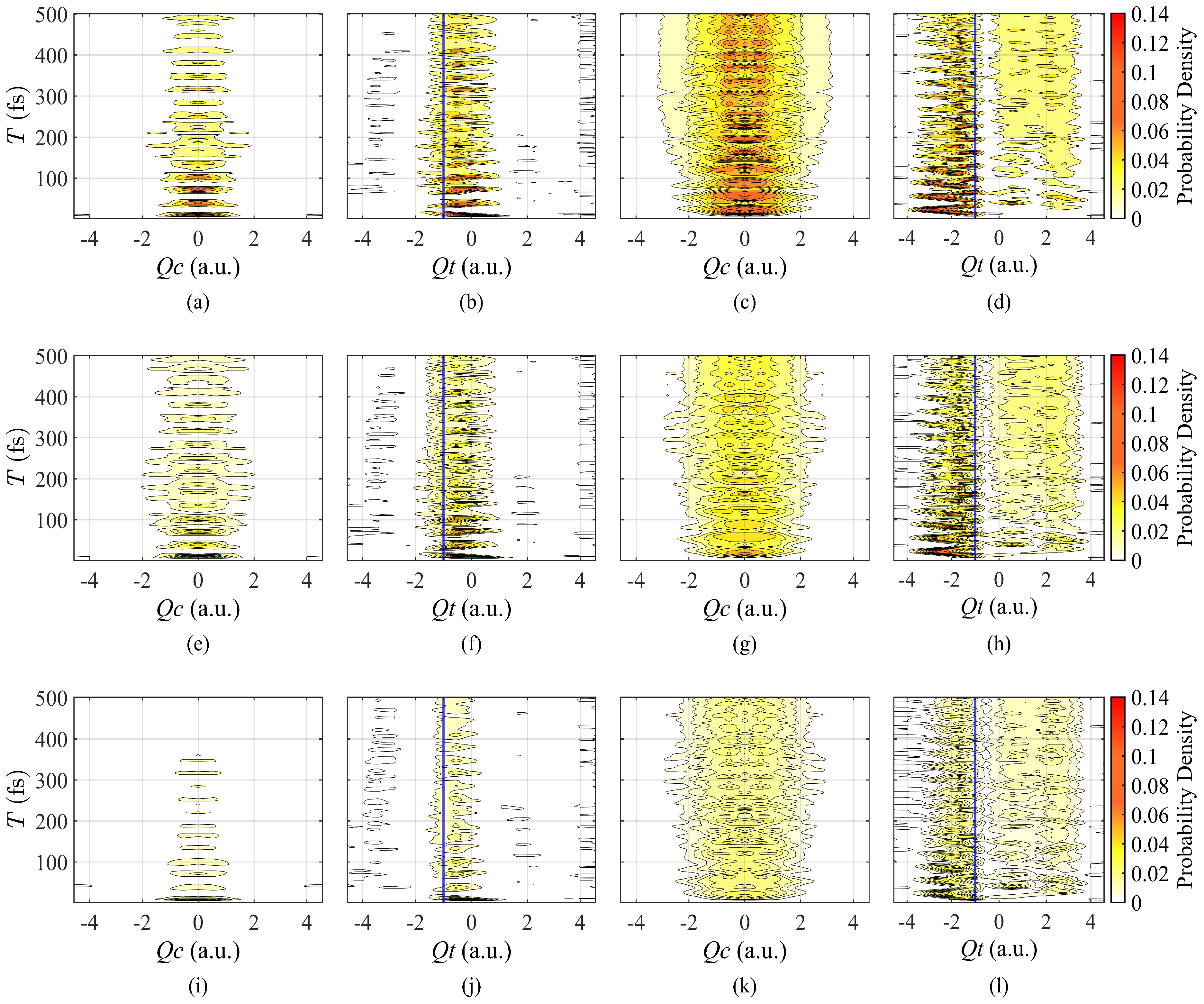
3.2. Pulse with Different Durations

We also study the impact of pulse duration on the quantum efficiency of the CI system. A comparison of wave packet dynamics for different durations is shown in Figure 6. Here, the 0.6−1−0.6 linear scenario is taken as an example.
Compared to amplitude modulation, the temporal offset modulation of the line shape sub-pulses provides more varied information. With increasing temporal offset, the differences in wave packet motion become increasingly pronounced. Observing the Q c pathway, besides a significant reduction in stimulated effects of the system, there is a gradual decrease in the distribution range of the wave packet on the two excited states, moving closer to the conical intersection point. In Figure 6a,e,i, a continuous decrease in the oscillation period on the second excited state with increasing temporal offset is observed, accompanied by accelerated decay. In Figure 6c,g,k, a notable concentration of the wave packet distribution on the first excited state along the coupling mode near the conical intersection point is observed. This indicates that the temporal offset modulation corresponding to this pulse waveform has a certain impact on the system’s dynamic evolution under the coupling mode. The same phenomenon is observable in the Q t pathway, where with increasing temporal offset, the rate of disappearance of system coherence increases. In Figure 6d, system coherence gradually disappears after 200 fs, whereas in Figure 6h,l, coherence is absent at 100 fs and 40 fs, respectively, indicating system stabilization in a very short time frame with a more uniform distribution on the first excited state. This suggests that under this waveform setting, temporal offset modulation has a certain degree of influence on the stimulated system’s quantum yield. According to our calculations, under the relative amplitude setting of 0.6−1−0.6, a temporal offset scenario of 2 fs corresponds to a quantum yield increase of 2.15%, while scenarios of 3 fs and 4 fs lead to increases of 5.63% and 5.96%, respectively. The variations in quantum yield differences with time offsets are supplemented in the various amplitude modulation scenarios in Figure 5 and Table 1. Our study demonstrates that the time offset modulation of waveform has a certain influence on the quantum effects of the system’s photoexcitation process.
As shown in Figure 6, significant differences in wave packet dynamics emerge as the time offsets of the sub-pulses’ central times increase. Observing the Q c pathway, it is evident that as the time offset increases, the excitation efficiency of the system significantly decreases, leading to a shortened convergence time. Meanwhile, under the Q t pathway, the distribution of the wave packet along the vibrational coordinates near the conical intersection point on the second excited state becomes closer, and the quantum yield on the first excited state increases.In Figure 5 and Table 1, we compared the differences in the quantum yield of the system after using composite Gaussian pulse excitation models with the standard model using a single Gaussian pulse. The variations in quantum yield differences with time offsets are supplemented in the various amplitude modulation scenarios in Figure 5 and Table 1. Our study demonstrates that the time offset modulation of the waveform has a certain influence on the quantum effects of the system’s photoexcitation process.

4. Discussion

In this paper, our research demonstrates the significant impact of laser pulse waveform on the excitation process. Previous experimental studies have employed various methods of composite sub-pulses to alter the pulse waveform, contrasting the photoexcitation effects of different waveforms. It has been observed in experiments that such manipulations exert a crucial influence on the quantum effects induced in the system, surpassing experimental error limits by a significant margin. Historically, the process of laser excitation of materials with different waveforms has been analyzed from a physical perspective, focusing on the effect of the laser’s instantaneous intensity variation over time on the process of electronic energy absorption. However, as of now, humanity lacks the capability to directly observe the ultrashort time physical process of electron energy absorption. Our study successfully simulated this process theoretically, observing coherent dynamical processes of excited states within ultrashort time frames and physical phenomena at points of PES degeneracy. According to our calculations, the waveform of laser pulses exhibits effects on the material excitation process that surpass experimental error margins, reflecting the need for further investigation into the ultrafast radiation and absorption mechanisms in the microscopic domain. Our work provides a factor influencing quantum effects for data analysis in future coherent optical experiments and offers a key perspective for understanding the process of electronic energy variation in future research endeavors. Moreover, the phase of pulse is also the other key factor to determine the efficiency in the vicinity of the CI. The impact of pulse phase and its interaction to the molecular electronic transitions can be further investigated.

5. Conclusions

We utilized a conical intersection (CI) structure model as our research subject and employed a composite of multiple Gaussian profiles to modify the waveform of laser pulses, determining the parameters involved in our calculations. By combining the perturbed matrix approach (PMA) and time non-local (TNL) theories, we simulated the laser excitation process and energy transfer within the system. The probability densities obtained from the calculations were projected onto two vibrational modes to visualize dynamic distribution information. Under both modulation methods, we observed the influence of laser pulses on the photoexcitation process and the system’s evolution. Furthermore, we quantified the specific impact level through calculating quantum yield.

Author Contributions

H.H. and H.D. conceived the research project and held discussions with Q.D.; Q.D. calculated the results; Q.D. and J.Y. wrote the first draft and all authors refined the manuscript. All authors have read and agreed to the published version of the manuscript.

Funding

We thank the Ningbo International Science and Technology Cooperation with No. 2023H009, Graduate Student Scientific Research and Innovation Project of Ningbo University and NSFC grant with No. 12274247 for financial support.

Institutional Review Board Statement

Not applicable.

Informed Consent Statement

Not applicable.

Data Availability Statement

Data are contained within the article.

Conflicts of Interest

The authors declare no conflicts of interest.

Appendix A

Appendix A.1. The Description of TNL

The Liouville–von Neumann equation:
W ( t ) ˙ = i [ H t o t , W ( t ) ] = L W ( t )
W ( t ) in the formula represents the overall density operator, and L represents the Liouville super operator of the entire system. According to the composition of the quantum system, H t o t = H S + H B + H S B can decompose L into
L = L S + L B + L SB
Among them, L S , L B and L SB , respectively, represent the Liouville super operator of the studied system, environmental thermal reservoir and system–environment interaction. The projection operator P is introduced to act on the overall density operator, that is, ρ ( t ) = P W ( t ) , where ρ ( t ) is the reduced density operator symbol. For the system expressed by Equation (A2), the projection operator in the thermal library degree of freedom includes a trace operator. By introducing the projection operator, the overall density operator can be decomposed into related terms ρ ( t ) and irrelevant items ( 1 P ) W ( t ) , that is
W ( t ) = ρ ( t ) + ( 1 P ) W ( t ) , P 2 = P
Through derivation and arrangement, the specific form of the main equation used in this article can be written as
ρ ( t ) ˙ = L S e f f ρ ( t ) + 0 t d t K ( t , t ) ρ ( t ) + Γ ( t )
L S e f f = L S + t r B L I ρ B e q + L r e n
K ( t , t ) = t r B L I ( T e t t d t ( 1 P ) L ) ( 1 P ) ( L B + L I ) ρ B e q
Γ ( t ) = t r B L I ( T e t t d t ( 1 P ) L ) ( 1 P ) W ( 0 )
In the formula, L S e f f ρ ( t ) , K ( t , t ) and Γ ( t ) represent reversible terms, memory terms and non-homogeneous terms, respectively. The total Hamiltonian of the system H = H S + H B + H I + H r e n , where H r e n is the renormalization term. Correspondingly, the Liouville super operators L S , L I and L r e n , respectively, correspond to the corresponding Hamiltonian operator. In addition, Γ represents a temporal operator, and L S e f f · = i [ H S + H r e n , · ] . Expanding the associated thermal equilibrium state ρ e q according to the first order under all coupling strength conditions, we obtain the following:
ρ e q 1 Z S 1 Z B e β ( H S + H B ) 1 Z S 1 Z B 0 β d β e ( β β ) ( H S + H B ) H 1 e β ( H S + H B )
The corresponding allocation function is Z i = t r i e x p ( β H i ) , i = B , S . The thermal equilibrium state of the environment can be written according to Formula (A8):
ρ B e q = 1 Z B e β H B + χ Z B 0 β d β e ( β β ) H B i = 1 N c i x i e β H B
χ = ( 1 / Z S ) t r S [ f ( x ) e β H S ] in the formula, f ( x ) represents the system–environment interaction form. The system–environment correlation function is
c ( t ) = d ω 2 π J ( ω ) cos ( ω t ) coth β ω 2 i d ω 2 π J ( ω ) sin ( ω t ) a ( t ) i b ( t )
Using a ( t ) and b ( t ) , we now rewrite Formulas (A5)–(A7):
L s e f f = L s + μ L r e n , s + χ μ L
K ( t , t ) = L a ( t t ) T e t t L s L + b ( t t ) T e t t L s L +
Γ ( t ) = L 0 d t a ( t t ) T e t t L s L ρ s e q + b ( t t ) T e t t L s L + ρ s e q
where L = i [ H s b , · ] and L + = [ H s b , · ] + 2 χ . Additionally, μ = d ω 2 π J ( ω ) / ω is given by the spectral density function.
We introduce the spectral density function of the parametric Ohmic spectrum as follows:
J ( ω ) = π 2 k = 1 n P k ω [ ( ω + Ω k ) 2 + Γ k 2 ] [ ( ω Ω k ) 2 + Γ k 2 ]
where P k , Ω k and Γ k are arbitrary real numbers, representing spectral amplitude, frequency and width, respectively. Any spectral density can be fitted using the above formula. And by bringing the spectral density function into the environmental correlation function, we obtain
a ( t ) = k = 1 n P k 8 Ω k Γ k coth β 2 ( Ω k + i Γ k ) e i Ω k t Γ k t + k = 1 n P k 8 Ω k Γ k coth β 2 ( Ω k i Γ k ) e i Ω k t Γ k t + 2 i β k = 1 n J ( i ν k ) e ν k t
b ( t ) = k = 1 n i P k 8 Ω k Γ k e i Ω k t Γ k t e i Ω k t Γ k t
Now, we define two auxiliary density matrices:
ρ k r ( t ) = λ T e 0 t d t L s e γ k r t 0 d t e L s t e γ k r t L ρ s e q + 0 t d t e γ k r ( t t ) T e t t L s L ρ s ( t )
ρ k i ( t ) = λ T e 0 t d t L s e γ k i t 0 d t e L s t e γ k i t L + ρ s e q + 0 t d t e γ k i ( t t ) T e t t L s L + ρ s ( t )
Using a ( t ) = k = 1 n r α k r e γ k r t and b ( t ) = k = 1 n i α k i e γ k i t to represent the correlation function, where n i = 2 n , n r = 2 n + n , and n is the number of Matsubara frequencies used, we obtain the final form of the time non-local quantum master equation:
ρ ˙ s ( t ) = L s e f f ( t ) ρ s ( t ) + λ k = 1 n r α k r L ρ k r ( t ) + k = 1 n i α k i L ρ k i ( t )
ρ ˙ k r ( t ) = L s ( t ) + γ k r ρ k r + λ L ρ s ( t ) , k = 1 , , n r
ρ ˙ k i ( t ) = L s ( t ) + γ k i ρ k r + λ L + ρ s ( t ) , k = 1 , , n i

Appendix A.2. Supplementary Information on Model Parameter Settings

In fact, in wave number units (cm−1), the gap between the electronic ground-state energy level and the second excited state is between 10,000 and 25,000 units. To improve calculation efficiency, we set Δ E to 2000 cm−1, but this does not affect the correctness of our calculation results. We calculated the wave packet dynamics images with Δ E of 2000 cm−1 (Figure A1) and 12,500 cm−1 (Figure A2), while other parameters remained constant. The two images show that the energy level difference between the electronic ground state and the second excited state has minimal effect on the excitation process.
Figure A1. Calculation results of wave packet dynamics under the Δ E = 2000 cm−1 scenario.
Photonics 11 00511 g0a1
Figure A2. Calculation results of wave packet dynamics under the Δ E = 12,500 cm−1 scenario.
Photonics 11 00511 g0a2

References

  1. Domcke, W.; Yarkony, D.R.; Koppel, H. Conical Intersection: Electronic Structure, Dynamics and Spectroscopy. In World Scientific; Domcke, W., Yarkony, D.R., Koppel, H., Eds.; World Scientific: Singapore, 2004. [Google Scholar]
  2. Domcke, W.; Yarkony, D.R.; Koppthe, H. Conical intersections: Theory, computation and experiment In World Scientific; Domcke, W., Yarkony, D.R., Koppel, H., Eds.; World Scientific: Singapore, 2011. [Google Scholar]
  3. Kowalewski, M.; Fingerhut, B.P.; Dorfman, K.E.; Bennett, K.; Mukamel, S. Simulating Coherent Multidimensional Spectroscopy of Nonadiabatic Molecular Processes. Infrared X-ray Regime Chem. Rev. 2017, 117, 12165–12226. [Google Scholar] [PubMed]
  4. Hoffman, D.P.; Mathies, R.A. Femtosecond Stimulated Raman Exposes the Role of Vibrational Coherence in Condensed-Phase Photoreactivity. Acc. Chem. Res. 2016, 49, 616–625. [Google Scholar] [CrossRef] [PubMed]
  5. Arimondo, E.; Orriols, G. Nonabsorbing atomic coherences by coherent two-photon transitions in a three-level optical pumping. Nuovo Cimento Lett. 1976, 17, 333–338. [Google Scholar] [CrossRef]
  6. Kowalewski, M.; Bennett, K.; Dorfman, K.E.; Mukamel, S. Catching conical intersections in the act: Monitoring transient electronic coherences by attosecond stimulated X-ray Raman signals. Phys. Rev. Lett. 2015, 115, 193003. [Google Scholar] [CrossRef] [PubMed]
  7. Jadoun, D.; Zhang, Z.; Kowalewski, M. Raman Spectroscopy of Conical Intersections Using Entangled Photons. J. Phys. Chem. Lett. 2024, 15, 2023–2030. [Google Scholar] [CrossRef] [PubMed]
  8. Polli, D.; Altoè, P.; Weingart, O.; Spillane, K.M.; Manzoni, C.; Brida, D.; Tomasello, G.; Orlandi, G.; Kukura, P.; Mathies, R.A.; et al. Conical intersection dynamics of the primary photoisomerization event in vision. Nature 2010, 467, 440–443. [Google Scholar] [CrossRef]
  9. Schnedermann, C.; Liebel, M.; Kukura, P. Mode-Specificity of Vibrationally Coherent Internal Conversion in Rhodopsin during the Primary Visual Event. Am. Chem. Soc. 2015, 137, 2886–2891. [Google Scholar] [CrossRef] [PubMed]
  10. Zinchenko, K.S.; Ardana-Lamas, F.; Seidu, I.; Neville, S.P.; van der Veen, J.; Lanfaloni, V.U.; Schuurman, M.S.; Wörner, H.J. Sub-7-femtosecond conical-intersection dynamics probed at the carbon K-edge. Science 2021, 371, 489–494. [Google Scholar] [CrossRef]
  11. Johnson, P.J.M.; Farag, M.H.; Halpin, A.; Morizumi, T.; Prokhorenko, V.I.; Knoester, J.; Jansen, T.L.; Ernst, O.P.; Miller, R.D. The Primary Photochemistry of Vision Occurs at the Molecular Speed Limit. J. Phys. Chem. B 2017, 121, 4040–4047. [Google Scholar] [CrossRef]
  12. Johnson, P.J.M.; Halpin, A.; Morizumi, T.; Prokhorenko, V.I.; Ernst, O.P.; Miller, R.D. Local vibrational coherences drive the primary photochemistry of vision. Nat. Chem. 2015, 7, 980–986. [Google Scholar] [CrossRef]
  13. Musser, A.J.; Liebel, M.; Schnedermann, C.; Wende, T.; Kehoe, T.B.; Rao, A.; Kukura, P. Evidence for conical intersection dynamics mediating ultrafast singlet exciton fission. Nat. Phys. 2015, 11, 352–357. [Google Scholar] [CrossRef]
  14. Duan, H.-G.; Jha, A.; Li, X.; Tiwari, V.; Ye, H.; Nayak, P.K.; Zhu, X.L.; Li, Z.; Martinez, T.J.; Thorwart, M.; et al. Intermolecular vibrations mediate ultrafast singlet fission. Sci. Adv. 2008, 6, abb0052. [Google Scholar] [CrossRef]
  15. Kukura, P.; McCamant, D.W.; Yoon, S.; Wandschneider, D.B.; Mathies, R.A. Structural Observation of the Primary Isomerization in Vision with Femtosecond-Stimulated Raman. Science 2005, 310, 1006–1009. [Google Scholar] [CrossRef] [PubMed]
  16. Kuramochi, H.; Tsutsumi, T.; Saita, K.; Wei, Z.; Osawa, M.; Kumar, P.; Liu, L.; Takeuchi, S.; Taketsugu, T.; Tahara, T. Ultrafast Raman observation of the perpendicular intermediate phantom state of stilbene photoisomerization. Nat. Chem. 2024, 16, 22–27. [Google Scholar] [CrossRef] [PubMed]
  17. Mandal, A.; Ziegler, L.D. Vibrational line shape effects in plasmon-enhanced stimulated Raman spectroscopies. J. Chem. Phys. 2021, 155, 194701. [Google Scholar] [CrossRef] [PubMed]
  18. Takeuchi, S.; Ruhman, S.; Tsuneda, T.; Chiba, M.; Taketsugu, T.; Tahara, T. Spectroscopic Tracking of Structural Evolution in Ultrafast Stilbene Photoisomerization. Science 2008, 322, 1073–1077. [Google Scholar] [CrossRef]
  19. Frontiera, R.R.; Mathies, R.A. Femtosecond stimulated Raman spectroscopy. Laser Photonics Rev. 2011, 5, 102–113. [Google Scholar] [CrossRef]
  20. Batignani, G.; Ferrante, C.; Scopigno, T. Accessing excited state molecular vibrations by femtosecond stimulated Raman spectroscopy. J. Phys. Chem. Lett. 2020, 11, 7805–7813. [Google Scholar] [CrossRef]
  21. Lynch, P.G.; Das, A.; Alam, S.; Rich, C.C.; Frontiera, R.R. Mastering Femtosecond Stimulated Raman Spectroscopy: A Practical Guide. ACS Phys. Chem. Au 2023, 4, 1–18. [Google Scholar] [CrossRef]
  22. Yang, J.; Zhu, X.; Wolf, T.J.; Li, Z.; Nunes, J.P.F.; Coffee, R.; Cryan, J.P.; Gühr, M.; Hegazy, K.; Heinz, T.F.; et al. Imaging CF3I conical intersection and photodissociation dynamics with ultrafast electron diffraction. Science 2018, 361, 64–67. [Google Scholar] [CrossRef]
  23. Chen, L.; Gelin, M.F.; Chernyak, V.Y.; Domcke, W.; Zhao, Y. Dissipative dynamics at conical intersections: Simulations with the hierarchy equations of motion method. Faraday Discuss. 2016, 194, 61–80. [Google Scholar] [CrossRef] [PubMed]
  24. González-Luque, R.; Garavelli, M.; Bernardi, F.; Merchán, M.; Robb, M.A.; Olivucci, M. Computational evidence in favor of a two-state, two-mode model of the retinal chromophore photoisomerization. Proc. Natl. Acad. Sci. USA 2000, 97, 9379–9384. [Google Scholar] [CrossRef]
  25. Krčmȧř, J.; Gelin, M.F.; Egorova, D.; Domcke, W. Signatures of conical intersections in two-dimensional electronic spectra. J. Phys. B 2014, 47, 124019. [Google Scholar] [CrossRef]
  26. Chen, L.; Gelin, M.F.; Zhao, Y.; Domcke, W. Mapping of Wave Packet Dynamics at Conical Intersections by Time- and Frequency-Resolved Fluorescence Spectroscopy: A Computational Study. J. Phys. Chem. Lett. 2019, 10, 5873–5880. [Google Scholar] [CrossRef] [PubMed]
  27. Qi, D.L.; Duan, H.G.; Sun, Z.R.; Miller, R.J.; Thorwart, M. Tracking an electronic wave packet in the vicinity of a conical intersection. J. Chem. Phys. 2017, 147, 074101. [Google Scholar] [CrossRef]
  28. Duan, H.G.; Qi, D.L.; Sun, Z.R.; Miller, R.D.; Thorwart, M. Signature of the geometric phase in the wave packet dynamics on hypersurfaces. Chem. Phys. 2018, 515, 21–27. [Google Scholar] [CrossRef]
  29. Duan, H.-G.; Thorwart, M. Quantum Mechanical Wave Packet Dynamics at a Conical Intersection with Strong Vibrational Dissipation. J. Phys. Chem. Lett. 2016, 7, 382–386. [Google Scholar] [CrossRef] [PubMed]
  30. Duan, H.-G.; Miller, R.J.D.; Thorwart, M. Impact of Vibrational Coherence on the Quantum Yield at a Conical Intersection. J. Phys. Chem. Lett. 2016, 7, 3491–3496. [Google Scholar] [CrossRef]
  31. Timmers, H.; Zhu, X.; Li, Z.; Kobayashi, Y.; Sabbar, M.; Hollstein, M.; Reduzzi, M.; Martínez, T.J.; Neumark, D.M.; Leone, S.R. Disentangling conical intersection and coherent molecular dynamics in methyl bromide with attosecond transient absorption spectroscopy. Nat. Commun. 2019, 10, 3133. [Google Scholar] [CrossRef]
  32. Keefer, D.; Freixas, V.M.; Song, H.; Tretiak, S.; Fernandez-Alberti, S.; Mukamel, S. Monitoring molecular vibronic coherences in a bichromophoric molecule by ultrafast X-ray spectroscopy. Chem. Sci. 2021, 12, 5286–5294. [Google Scholar] [CrossRef]
  33. Hosseinizadeh, A.; Breckwoldt, N.; Fung, R.; Sepehr, R.; Schmidt, M.; Schwander, P.; Santra, R.; Ourmazd, A. Few-fs resolution of a photoactive protein traversing a conical intersection. Nature 2021, 599, 697–701. [Google Scholar] [CrossRef]
  34. Yang, J.; Zhu, X.F.; Nunes, J.P.; Yu, J.K.; Parrish, R.M.; Wolf, T.J.; Centurion, M.; Gühr, M.; Li, R.; Liu, Y.; et al. Simultaneous observation of nuclear and electronic dynamics by ultrafast electron diffraction. Science 2020, 368, 885–889. [Google Scholar] [CrossRef]
  35. Nam, Y.; Keefer, D.; Nenov, A.; Conti, I.; Aleotti, F.; Segatta, F.; Lee, J.Y.; Garavelli, M.; Mukamel, S. Conical Intersection Passages of Molecules Probed by X-ray Diffraction and Stimulated Raman Spectroscopy. J. Phys. Chem. Lett. 2021, 12, 12300–12309. [Google Scholar] [CrossRef] [PubMed]
  36. von Conta, A.; Tehlar, A.; Schletter, A.; Arasaki, Y.; Takatsuka, K.; Wörner, H.J. Conical-intersection dynamics and ground-state chemistry probed by extreme-ultraviolet time-resolved photoelectron spectroscopy. Nat. Commun. 2018, 9, 3162. [Google Scholar] [CrossRef] [PubMed]
  37. Prokhorenko, V.I.; Nagy, A.M.; Waschuk, S.A.; Brown, L.S.; Birge, R.R.; Miller, R.D. Coherent control of retinal isomerization in bacteriorhodopsin. Science 2006, 313, 1257–1261. [Google Scholar] [CrossRef] [PubMed]
  38. Xie, X.; Doblhoff-Dier, K.; Roither, S.; Schöffler, M.S.; Kartashov, D.; Xu, H.; Rathje, T.; Paulus, G.G.; Baltuška, A.; Gräfe, S.; et al. Attosecond-recollision-controlled selective fragmentation of polyatomic molecules. Phys. Rev. Lett. 2012, 109, 243001. [Google Scholar] [CrossRef] [PubMed]
  39. Levin, L.; Skomorowski, W.; Rybak, L.; Kosloff, R.; Koch, C.P.; Amitay, Z. Coherent control of bond making. Phys. Rev. Lett. 2015, 114, 233003. [Google Scholar] [CrossRef]
  40. Cerullo, G.; Bardeen, C.J.; Wang, Q.; Shank, C.V. High-power femtosecond chirped pulse excitation of molecules in solution. Chem. Phys. Lett. 1996, 262, 362–368. [Google Scholar] [CrossRef]
  41. Batignani, G.; Sansone, C.; Ferrante, C.; Fumero, G.; Mukamel, S.; Scopigno, T. Excited-state energy surfaces in molecules revealed by impulsive stimulated Raman excitation profiles. J. Phys. Chem. Lett. 2021, 12, 9239–9247. [Google Scholar] [CrossRef]
  42. Batignani, G.; Mai, E.; Fumero, G.; Mukamel, S.; Scopigno, T. Absolute excited state molecular geometries revealed by resonance Raman signals. Nat. Commun. 2022, 13, 7770. [Google Scholar] [CrossRef]
  43. May, V.; Kühn, O. Charge and Energy Transfer Dynamics in Molecular Systems; John Wiley and Sons: Hoboken, NJ, USA, 2023. [Google Scholar]
  44. Gelin, M.F.; Egorova, D.; Domcke, W. Efficient method for the calculation of time- and frequency-resolved four-wave mixing signals and its application to photon-echo spectroscopy. J. Chem. Phys. 2005, 123, 164112. [Google Scholar] [CrossRef] [PubMed]
  45. Gelin, M.F.; Egorova, D.; Domcke, W. Optical N-Wave-Mixing Spectroscopy with Strong and Temporally Well-Separated Pulses: The Doorway-Window Representation. J. Phys. Chem. B 2011, 115, 5648–5658. [Google Scholar] [CrossRef] [PubMed]
  46. Kleinekathöfer, U. Non-Markovian theories based on a decomposition of the spectral density. J. Chem. Phys. 2004, 121, 2505–2514. [Google Scholar] [CrossRef] [PubMed]
  47. Meier, C.; Tannor, D.J. Non-Markovian evolution of the density operator in the presence of strong laser fields. J. Chem. Phys. 1999, 111, 3365–3376. [Google Scholar] [CrossRef]
Figure 1. A schematic of potential energetic surfaces of coupling (a) and tuning modes (b). The electronic states are coupled to the two modes, Q c and Q t .
Photonics 11 00511 g001
Figure 2. The wave packet dynamics of excited state e 2 and e 1 along Q c and Q t : (a) P 2 a d ( Q c , t ) , (b) P 2 a d ( Q t , t ) , (c) P 1 a d ( Q c , t ) and (d) P 1 a d ( Q t , t ) .
Photonics 11 00511 g002
Figure 3. Comparison between single Gaussian (blue solid line) and composite Gaussian line shapes (red dashed line).
Photonics 11 00511 g003
Figure 4. Comparison of wave packet dynamics between single Gaussian line shape (ad) and 0.6−0.6−1 waveform (eh) configuration.The images in each row are consistent with Figure 2.
Photonics 11 00511 g004
Figure 5. Comparison of composite Gaussian line shape (red dashed line) and single Gaussian line shape (blue solid line) under various amplitude modulations.
Photonics 11 00511 g005
Figure 6. Comparison of wave packet dynamics for sub-pulses with different durations—2 fs (ad), 3 fs (eh), 4 fs (il). The images in each row are consistent with Figure 2.
Photonics 11 00511 g006
Table 1. The difference in quantum yield (DQY) of the same single Gaussian line type (Figure 5 blue solid line) under different durations for various line types (Figure 5 red dashed line).
DQY Duration2 fs3 fs4 fs
Pulse Shape
Line type 12.43%5.03%6.83%
Line type 23.38%6.88%3.92%
Line type 32.15%4.46%6.77%
Line type 42.80%5.63%5.96%
Line type 53.80%6.98%2.41%
Line type 61.55%2.30%1.26%
Line type 71.09%2.06%3.00%
Line type 81.82%3.44%4.68%
Disclaimer/Publisher’s Note: The statements, opinions and data contained in all publications are solely those of the individual author(s) and contributor(s) and not of MDPI and/or the editor(s). MDPI and/or the editor(s) disclaim responsibility for any injury to people or property resulting from any ideas, methods, instructions or products referred to in the content.

