Abstract
A vehicle-mounted solar occultation flux–Fourier transform infrared spectrometer uses the sun as an infrared light source to quantify molecular absorption in the atmosphere. It can be used for the rapid three-dimensional monitoring of pollutant emissions and the column concentration monitoring of greenhouse gases. The system has the advantages of high mobility and a capacity for noncontact measurement and measurement over long distances. However, in vehicle-mounted applications, vehicle bumps and obstacles introduce aberrations in the measured spectra, affecting the accuracy of gas concentration inversion results and flux calculations. In this paper, we propose a spectral data preprocessing method that combines a self-organizing mapping neural network and correlation analysis to reject anomalous spectral data measured by the solar occultation flux–Fourier transform infrared spectrometer during mobile observations. Compared to the traditional method, this method does not need to adjust the comparison threshold and obtain the training spectra in advance and has the advantage of automatically updating the weights without the need to set fixed correlation comparison coefficients. The accurate identification of all anomalous simulated spectra in the simulation experiments proved the effectiveness of the method. In the vehicle-mounted application experiment, 342 anomalous spectra were successfully screened from 1739 spectral data points. The experimental results show that the method can improve the accuracy of gas concentration measurement results and can be applied to a vehicle-mounted solar occultation flux–Fourier transform infrared spectrometer system to meet the preprocessing needs of a high number of spectral data in mobile monitoring.
1. Introduction
Solar spectrum analysis is a commonly used method in atmospheric research; the sun is used as a light source to quantify molecular absorption in the atmosphere and subsequently determine the concentration of trace gases [1]. The SOF–FTIR is an optical remote sensing technique that uses a Fourier transform infrared spectrometer (FTIR) in conjunction with a mobile solar tracking system, which is suitable for monitoring the spatial and temporal distributions of emissions on a large scale in a mapped city [2]. The SOF–FTIR is mounted on a vehicle that moves in a circle around the target pollution source, and the solar spectrum is extracted from the measured interferograms via a Fourier integral transform to determine the gas emissions from the source [3].
However, when cloud and building shadows are present in mobile ground monitoring, the solar intensity changes greatly and the amplitude of the interferogram decreases, leading to a reduction in the spectral signal-to-noise ratio [4]. The second vehicle bumps, the car turns quickly, and other factors affecting the FTIR within the solar beam jitter, causing misalignment in the optical path. On the one hand, this leads to the infrared detection of the size, location, and intensity of the changes, reducing the signal-to-noise ratio; on the other hand, it results in the expansion of the angle of incidence, resulting in spectral spread and drift, which directly affect the instrument line function. This, in turn, affects the spectral quality and accuracy of the inversion of the gas concentration [5]. Therefore, rejecting the measured error of the spectral data can reduce the error in the spectral inversion results.
To date, most efforts have been devoted to improving the spectrometer and the solar tracking system [6,7]; however, rectifying low-quality spectra remains a key challenge. Continuous mobile monitoring produces approximately 1 spectral data point per 4 s, while continuous monitoring produces more than 900 spectral data points per hour. The percentage of invalid interferometric data can be more than 50% when traveling in areas with poor conditions, such as cities with tall buildings [8]. The traditional spectral rejection method mainly uses the Spearman correlation between the measured spectrum and the standard spectrum to achieve the rejection of the spectral data [9]; however, it is very difficult to achieve the spectral rejection of the attenuated intensity with an insignificant absorption structure. The selection of correlation coefficients is also a key challenge. The infrared spectrum has many absorption peaks, and the Levenberg–Marquardt optimization algorithm [10] and the classic climbing algorithm [11] tend to fall into local optimal solutions when there are multiple peaks; thus, they may not be able to find the global optimal solution. The classic least squares algorithm [12] is very sensitive to outliers. Due to the harsh conditions of in-vehicle applications, complex, abnormal data may appear, which may lead to model instability.
Neural networks offer another method for spectrum suppression. Neural networks simulate the intelligent activities of the human brain by developing appropriate learning algorithms. The features include massively parallel processing, distributed storage, elastic topology, high redundancy, and nonlinear operation. They offer high computational speed, strong association abilities, strong adaptability, strong fault tolerance, and self-organization abilities [13]. To reject abnormal target values, researchers in other fields have proposed improved methods from an algorithmic point of view. Yuan et al. utilized the spectral difference between the abnormal target and the background, as well as the spatial sparsity of the abnormal target, to achieve anomaly detection in spectral data based on a fast robust anomaly detection algorithm [14]. Ma K et al. used deep neural networks to learn spectral and temporal features and a deep learning method to detect changes in the system caused by system disturbances in order to achieve anomaly detection in hyperspectral images [15]. Therefore, the application of neural networks to anomalous data processing is an effective method. When directly applying the deep learning method to anomaly detection in spectral data, it is impossible to provide a perfect training criterion because the SOF–FTIR spectral intensity changes with the intensity of solar irradiance.
However, neural network clustering methods do not require a standard learning spectrum in advance. We only need to specify the number of categories for classification, and the algorithm will classify all samples according to the similarity principle. The SOM network is an important example of a neural network based on unsupervised learning methods. It was first proposed in 1981 by Kohonen, a neural network expert at the Helsinki College of Technology, Finland. The results are relatively easy to visualize and interpret [16]. This technique has been shown to be effective in solar cell design, using structured feature agglomerative clustering as an unsupervised dimensionality reduction step to identify the main features of the spectrum, which can reduce datasets from thousands of solar spectra to several characteristic surrogate spectra. The network successfully used these surrogate spectra to predict annual average efficiency as a function of solar cell design [17].
In this paper, we propose a method for preprocessing the data from a vehicle-mounted Fourier transform infrared spectrometer to solve the above problems; we successfully applied this method to eliminate abnormal spectral data from a vehicle-mounted SOF–FTIR. In this article, first, the causes of abnormal spectra are analyzed, the principle of the SOM method is introduced, and a spectral data preprocessing method combining the SOM neural network and correlation analysis is proposed. The working principle of spectral rejection based on this method and the practical effect of spectral rejection, which solve the problem of selecting correlation comparison coefficients, are also proposed. Second, the effectiveness of the proposed spectral data preprocessing method is verified using simulated spectra. Third, the validity of the spectral data rejection method for the spectral data preprocessing method in mobile SOF–FTIR monitoring is verified. Finally, some conclusions are drawn in the Conclusion section.
2. Spectral Data Preprocessing Methods
2.1. Spectral Anomaly Cause Analysis
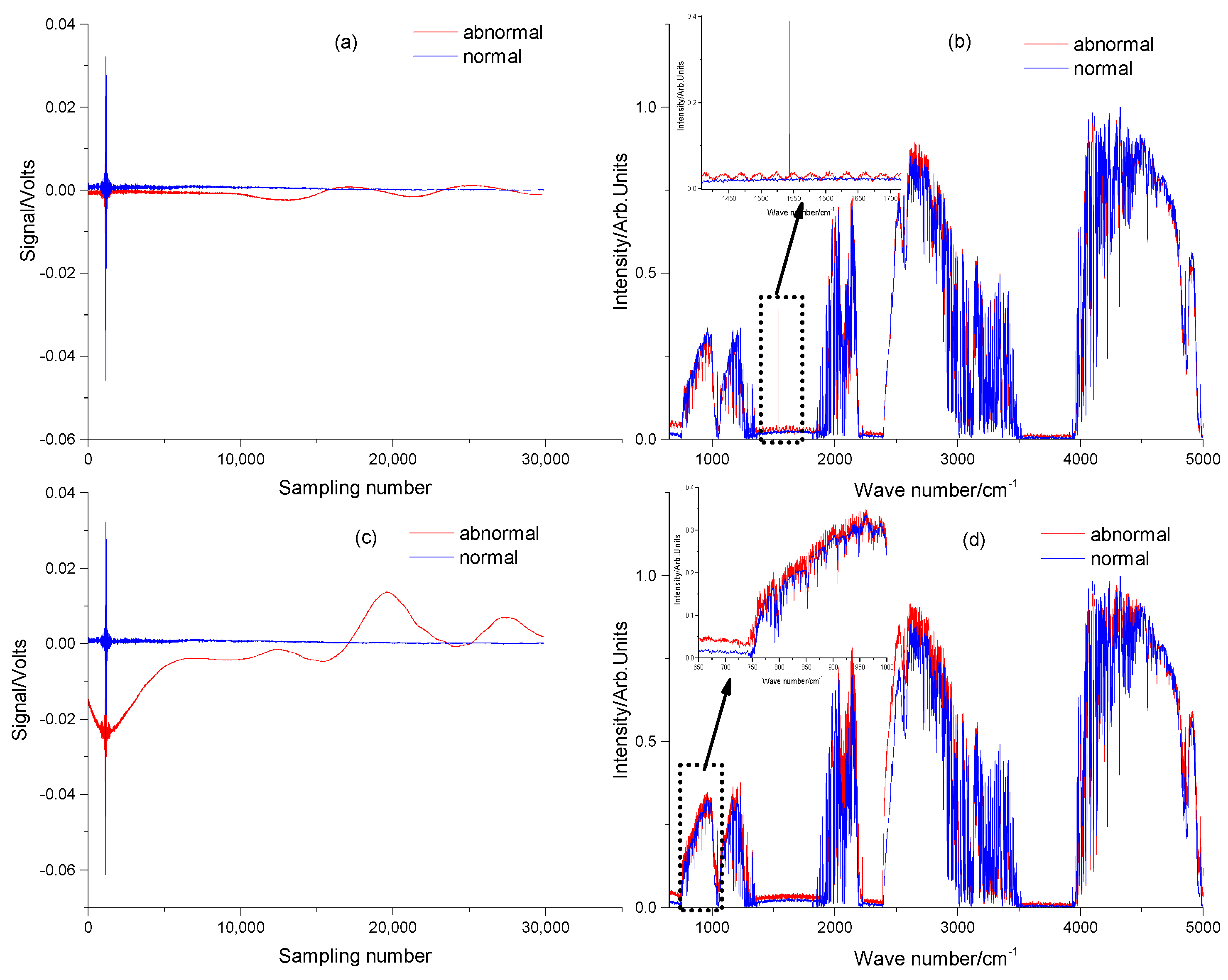
The simplest type of spectral anomaly in vehicle-mounted SOF–FTIR applications is low intensity in the center of the interferogram (at an optical range difference of zero), which is a deviation due to the sun being obscured by obstructions such as clouds or tree shadows. In our study, the intensity of the interferogram decreased by a factor of approximately 100 in clear weather when the incident optical path was completely obscured (Figure 1a,b). A lower intensity in the center of the interferogram leads to a lower calculated spectral amplitude in the single beam, which does not necessarily lead to errors in the measurement results when concentration calculations are performed on the spectral fit (Figure 1c,d). Therefore, it is not desirable to use the intensity at the center of the interferogram to reject anomalous data.
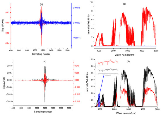
Figure 1.
Interference patterns and spectral patterns under different conditions. (a) Interference patterns under clear and blocked conditions. (b) Spectral patterns under clear and blocked conditions. (c) Interference patterns under different illumination intensities. (d) Spectral patterns under different illumination intensities (enlarged image shows that different light intensities do not affect the appearance of absorption structures).
Second, the low-frequency components caused by the vibration of one or more optical components during the use of a SOF–FTIR in vehicle-mounted systems due to vehicle shock, engine vibration, and wind, as well as electrical interference from the vehicle power supply, are included in the interferogram, which can result in an anomalous peak in the interferogram or oscillations that can lead to upward-emitting peaks or sinusoidal oscillations in the absorption spectrum. The further the peak is from the mean intensity of the interferogram, the higher the frequency of the oscillation. Figure 2 shows that single-beam spectra are affected due to incorrect spectral fitting results from superimposed emission peaks and oscillations in these spectra. However, we used a detector with an effective bandwidth of 650 cm−1~5000 cm−1, and any frequency perturbation outside the absorption band had no negative influence on the calculation of the gas absorption. Therefore, it was more effective to directly discard the spectral data within the effective band.
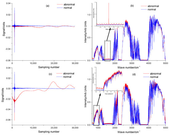
Figure 2.
Disturbed interferogram and the corresponding single-beam spectrum. (a) Interference pattern with fixed interference frequency superimposed. (b) Spectral pattern with fixed interference frequency superimposed (image enlarged to highlight the effect of interference on the spectrum). (c) Interference pattern with vibration interference superimposed. (d) Vibration interference-overlaid spectrum (image enlarged to highlight the impact of interference on the spectrum).
2.2. Data Preprocessing Methods
The SOM accepts an n-dimensional vector as input, which corresponds to an input layer with m nodes. The nodes of the input layer are connected to the competing layer via weight vectors, and each input sample corresponds to a node in the competing layer. When the training is completed, the input samples corresponding to the same node of the competing layer are classified into the same category [18]. The SOM includes an input layer and an output layer. The winning neuron of the SOM influences its neighboring neurons from near to far and gradually switches from excitation to inhibition. Therefore, not only does the winning neuron itself need to adjust the weight vector in its learning algorithm but the neurons around it also need to adjust the weight vector under its influence.
We obtained spectral data samples and normalized the individual spectral data to form an mxn multidimensional data matrix. Here, m represents the number of neurons for each spectral dataset, and n represents the number of spectral data samples.
We created a self-organizing mapping network model and set the weight vector between the input and output neurons to to form the neural network model.
We also created a self-organizing mapping network model and defined the weight vector between the input and output neurons as the composition of the neural network model.
Network training was also performed using the input spectral data and the nearest neuron was found via iterative training. The method used to calculate the distance is the Euclidean distance, and the expression for the Euclidean distance is shown in (2). The closer the weights are to the neuron, the smaller the distance.
In the SOM algorithm, not only does the winning neuron itself have to adjust the weight vector but so do the neurons in its vicinity. After the nearest neuron was found based on the Euclidean distance, the learning rate and neighborhood size parameters of the current iteration number were calculated to determine the neighborhood area. We updated the weight vectors of all neurons within the domain.
α is the learning rate; 0 < α ≤ 1. α generally decreases with the learning progress; that is, the degree of adjustment becomes smaller and smaller, tending toward the cluster center.
We determined whether the maximum number of iterations had been reached. If not, we continued the iterative training. After the training of the network was completed, each spectrum was inputted into the neural network, and each spectrum corresponded to an output neuron to obtain the results of spectral classification (Figure 3).
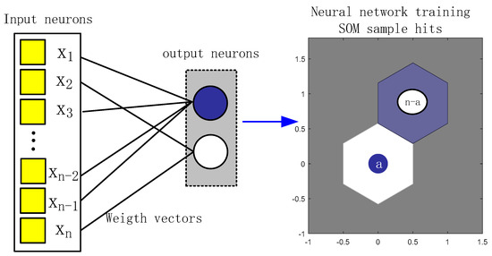
Figure 3.
Flowchart of the SOM calculation.
We performed a linear correlation analysis between the average spectrum of the classification result and the standard spectrum, and the spectrum with the highest correlation was the effective spectrum. The correlation coefficient is a measure of the close relationship between variables. Equation (6) is the expression for the correlation coefficient.
where S represents the standard spectral intensity and M represents the average spectral intensity of the classification results.
3. Preprocessing Experiments for Simulated Spectra
3.1. Simulation of Abnormal Spectra
The sunlight falls on the spectrometer through the sun-tracking system, and the complex color light interference signal formed by the Michelson interferometer is received by the infrared detector. The relationship between the interference signal and the complex color light can be expressed as Equation (7):
where ν is the wavenumber, x is the optical distance difference, and 2I0 is the DC component of the interferometric signal. The AC signal in the spectral measurement is the effective interferogram (Figure 4a).
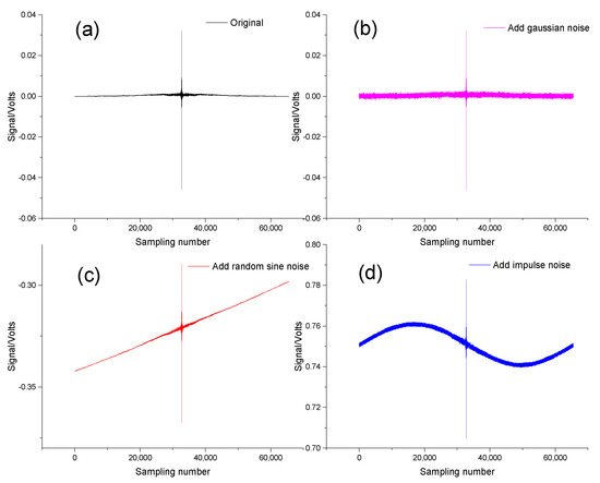
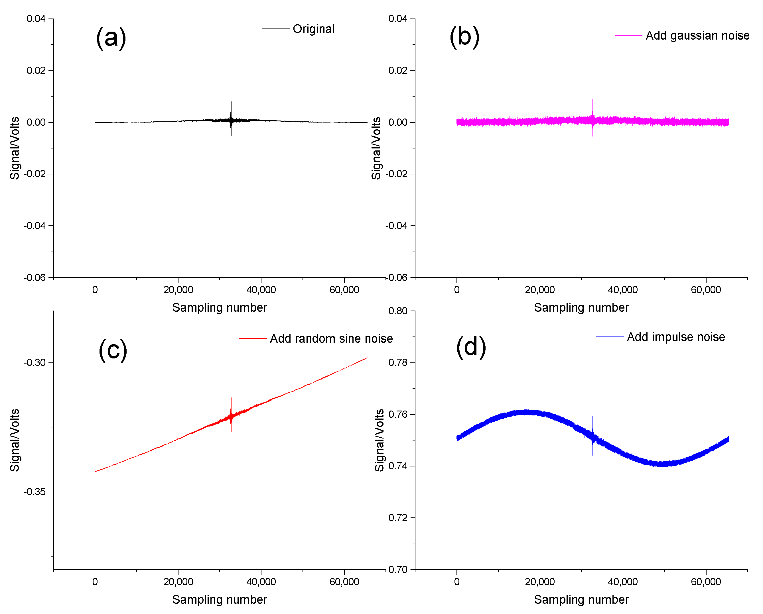
Figure 4.
Simulated interferogram. (a) Original interference signal. (b) Superimposed sinusoidal interference signal with a fixed frequency. (c) Superimposed interference signal with Gaussian noise. (d) Superimposed random sinusoidal interference signal.
To simulate measurement conditions such as vehicle-mounted random vibrations, a random variable η(N) with a noise intensity S, a mean value of 0, a variance of 1, and a Gaussian distribution was added to the interferogram to obtain a simulated interferogram with Gaussian noise (Figure 4b).
To simulate measurement conditions, such as low-frequency components caused by the vibration of one or more optical components due to vehicle unevenness, engine vibration, wind, and electrical interference from the vehicle’s power supply, random sinusoidal (Figure 4c) noises with a fixed frequency were added to the interferograms, and simulated interferograms with the addition of sinusoidal noises were obtained.
where A, f, and φ are the amplitude, frequency, and phase of the sinusoidal noise, respectively.
To simulate fluctuations in incident light caused by vehicle bumps and wind, we added sinusoidal impact interference noise to the interference data (Figure 4d).
where u(t) is the unit step function (Heaviside function), t0 is the starting time, T is the duration, and B is the amplitude.
Equation (12) represents the computational relationship between the spectrogram and the interferogram. In Fourier transform spectroscopy, the spectral information in the frequency domain is obtained from the output signal of the measurement in the time domain, and the recovered spectrum in the frequency domain is denoted by . Figure 5 shows the interferograms with various interfering noises and the corresponding single-beam spectra.
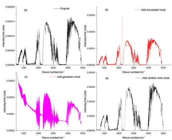
Figure 5.
Simulated spectrogram. (a) Original spectrogram. (b) Superimposed sinusoidal spectrogram with a fixed frequency. (c) Superimposed spectrogram with Gaussian noise. (d) Superimposed random sinusoidal spectrogram.
3.2. Experimental Results and Analysis
MATLAB software (R2016b) was used to simulate 51 abnormal spectra and 49 effective solar spectra with different amplitudes and frequencies, forming a 10,160 × 100 multidimensional spectral data matrix to test the performance of the spectral data preprocessing method. The dataset consisting of 100 spectra was classified using an SOM. The neuron positions and 100 spectral datasets in the topology of the SOM are shown in Figure 6a, assigned to two neurons with maximum hits of 51 and 49. The correlation coefficients between the average and standard spectra of the spectral datasets in each neuron were calculated. The class with a high correlation is the valid spectra, and the other class is the abnormal spectra. From the SOM calculation results, we can see that the neuron input spectra with a correlation coefficient of 0.999 are effective and the neuron input spectra with a correlation coefficient of 0.878 are abnormal. Based on a spectral data preprocessing method combining the SOM neural network and the correlation analysis proposed in this paper, all the emulated abnormal spectra were successfully identified in the classification results. According to the results of the correlation calculation, all three abnormal spectra are strongly correlated with the standard spectra. The spectral data preprocessing method proposed in this paper, which combines the SOM neural network and correlation analysis, avoids the difficulty of automatically distinguishing abnormal spectra with higher correlation due to the inappropriate selection of threshold parameters for correlation judgment, thereby affecting the accuracy of gas concentration inversion.
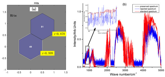
Figure 6.
Results of simulated spectral screening experiments. (a) Number of neuronal hits and correlation coefficients with standard spectra. (b) Comparison of neuronal mean spectra with standard spectra.
4. Data Acquisition and Processing
4.1. Experimental Instruments
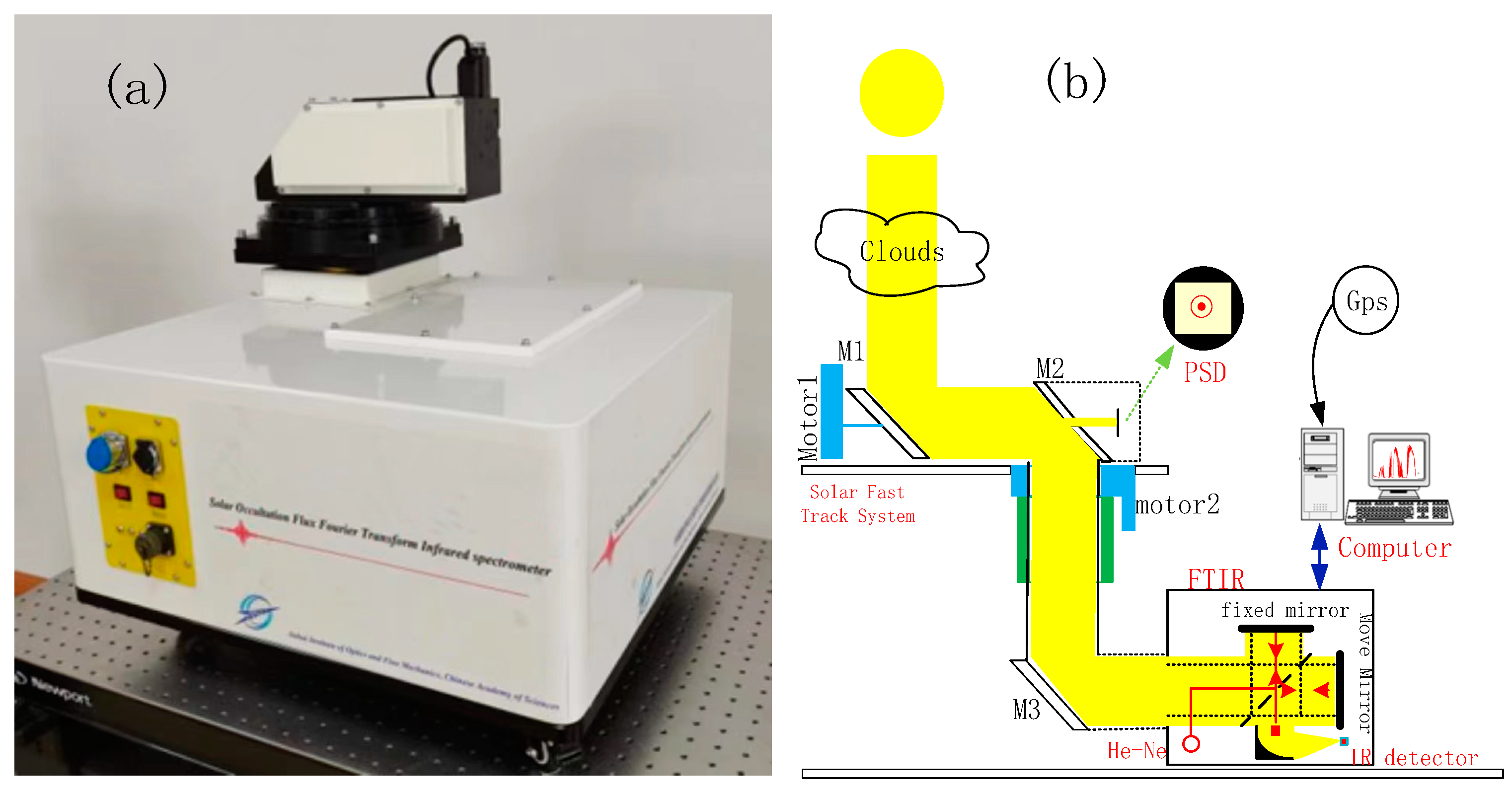
The SOF–FTIR system (Model AG-FTIR-SOF2000) included a solar tracking system (Figure 7a), a Global Positioning System (GPS) module, an FTIR spectrometer, and a computer (Figure 7b). We calculated the altitude and azimuth angle based on the GPS longitude and latitude information, roughly calculated the sun’s position, and used a position-sensitive detector to accurately record the changes in the sun’s position [19]. The solar spectra were obtained via the Fourier integral transformation of the measured interferograms and were used for the qualitative and quantitative analysis of the morphology of various substances.

Figure 7.
SOF–FTIR structure diagram. (a) SOF–FTIR system; (b) SOF-FTIR system structure diagram.
4.2. Data Acquisition
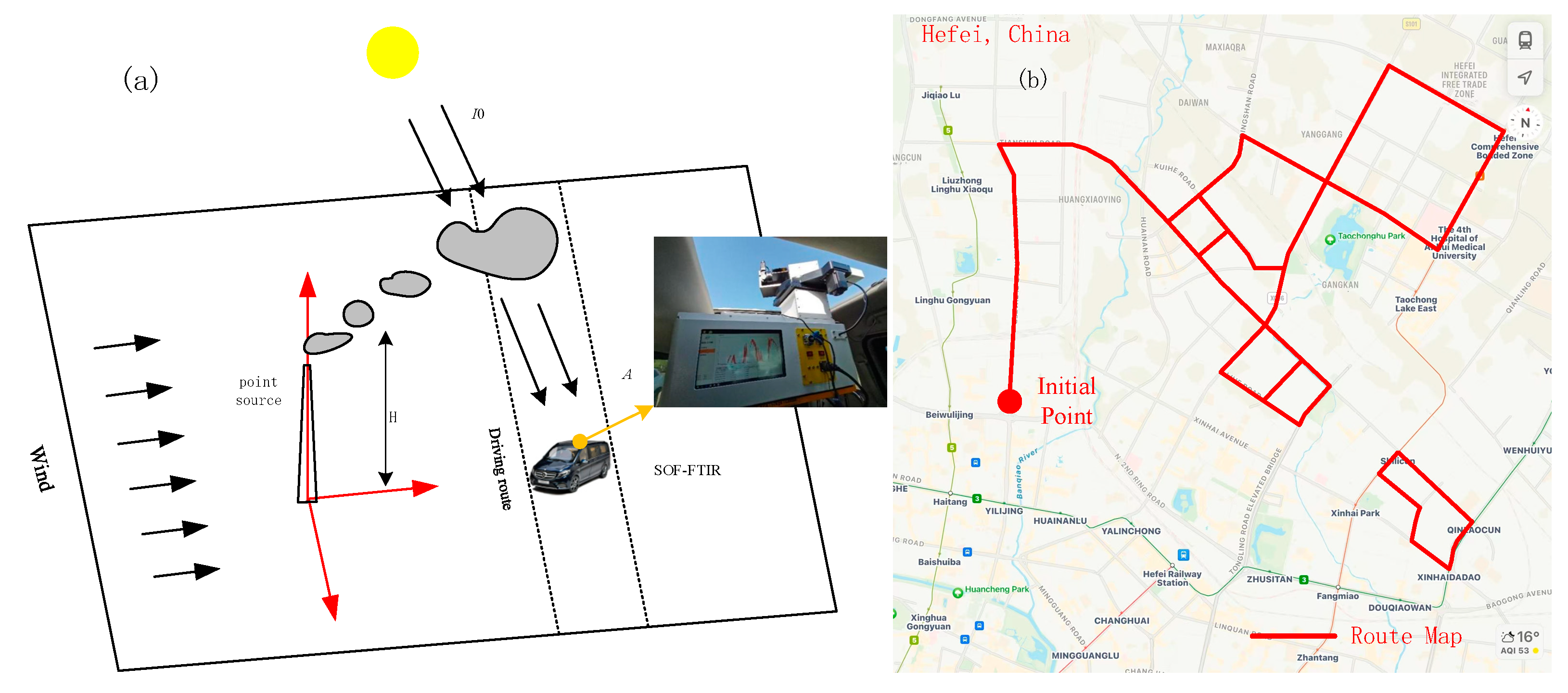
Vehicle-mounted SOF–FTIR observations of NH3 were conducted at an industrial park in Hefei City to verify the accuracy of the SOM-based data preprocessing method. The park mainly includes companies in the fields of video, photoelectrics, photovoltaics, liquid crystal glass, and new materials. For the mobile SOF–FTIR observation, sunlight selectively absorbed by the plume entered the FTIR spectrometer via the solar tracker (Figure 8).
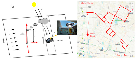
Figure 8.
Mobile monitoring experiment. (a) Schematic of vehicle-mounted SOF–FTIR monitoring. (b) Roadmap tracker.
The SOF–FTIR instrument lifted the solar track head out of the top of the vehicle via the lifting platform (Figure 8). The tracking vehicle traveled around the factory at an average speed of 40 km/h in a straight line and at a maximum speed of 20 km/h in curves.
4.3. Analysis of the Experimental Results
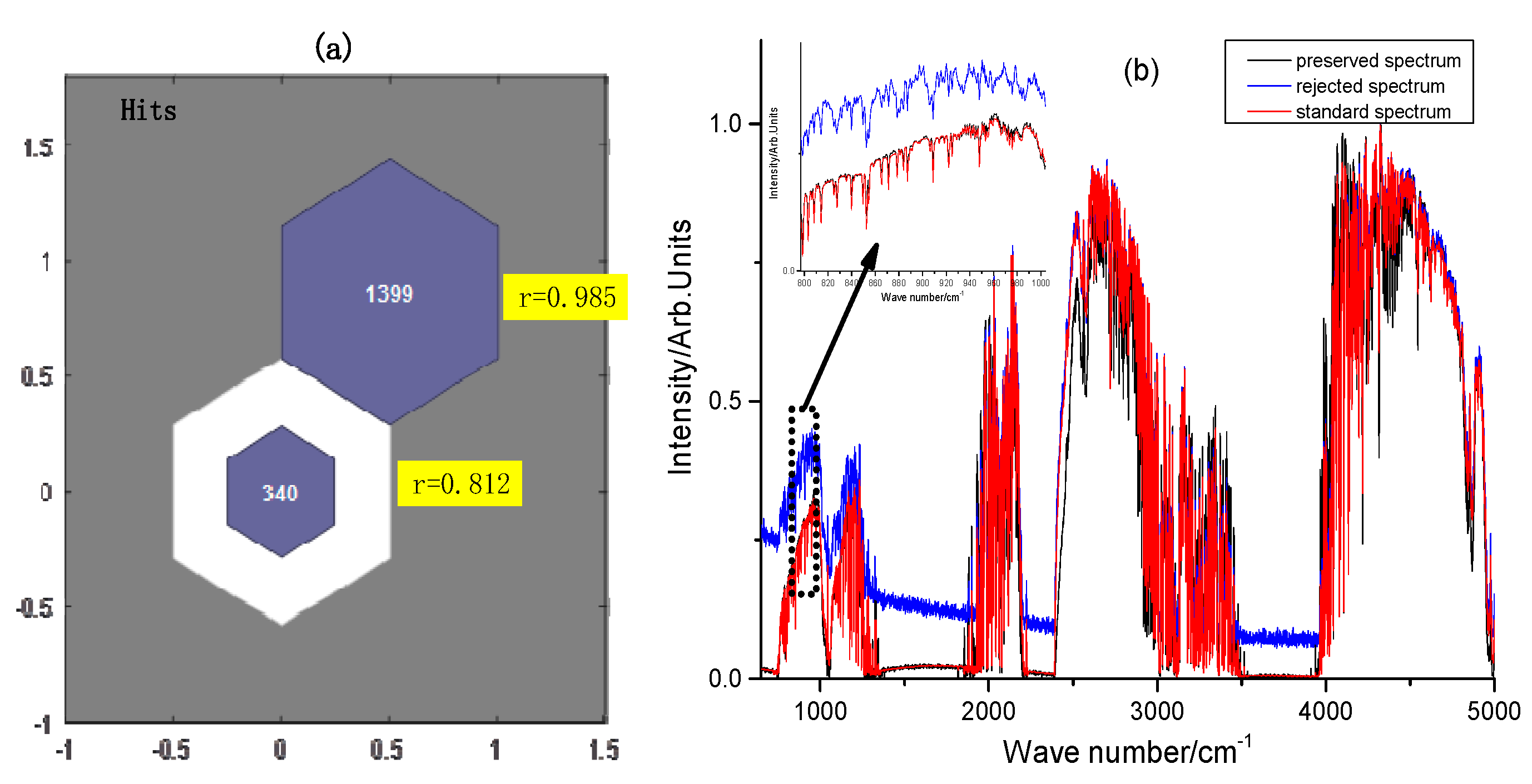
The 1739 spectral data points measured during mobile monitoring were summarized in a 10,160 × 1739 multidimensional spectral data matrix. The SOM was used to classify the dataset comprising the 1739 spectra. The neuron positions in the topology of the SOM and the 1739 spectral datasets are shown in Figure 9a and assigned to two neurons, where the maximum number of hits for the two neurons is 1399 and 340. We calculated the correlation coefficients between the average and standard spectra from the spectral datasets for each neuron. The class with high correlation is the effective spectrum, and the other class is the abnormal spectrum (Figure 9b). From the results of the SOM calculation, we can see that the neuron input spectra with a correlation coefficient of 0.938 are effective and those with a correlation coefficient of 0.812 are abnormal.

Figure 9.
Results of spectral screening experiments for vehicle applications. (a) Number of neuron hits and correlation coefficients with standard spectra. (b) Comparison of neuron average spectra with standard spectra.
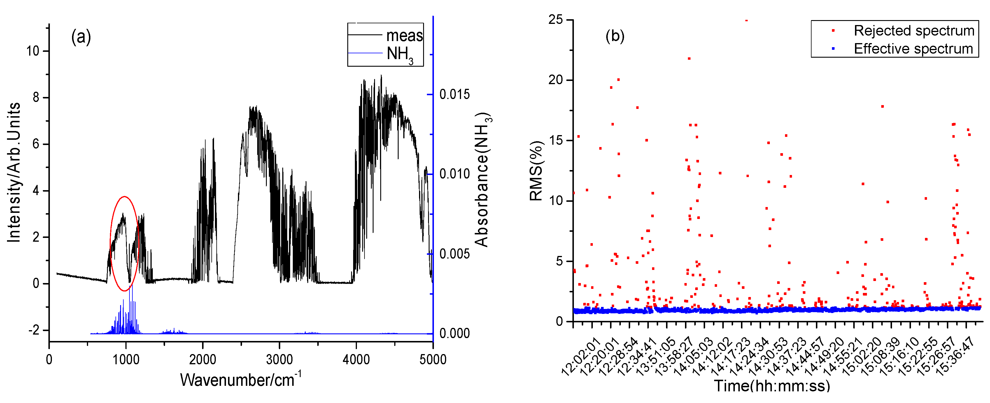
We selected the absorption cross-section for NH3 from the HITRAN and OAsoft databases and performed nonlinear least squares fit, along with the instrument parameters, to calculate the concentration of the pollutant. The 915 cm−1~980 cm−1 band with less interference from water vapor and carbon dioxide was selected for analysis. The transmission absorption spectrum in the corresponding area of the infrared transmission spectrum showed a consistent absorption pattern (Figure 10a). In the stationary analysis, the concentration of the transmission spectrum was inverted and fitted using the least squares method. The average RMS of the rejected spectrum fitting residuals was 4.28%, and the average RMS of the effective spectrum fitting residuals was 0.95% (Figure 10b).

Figure 10.
Analysis of the characteristic spectral bands of NH3 to be measured. (a) Measured spectra and NH3 integral line intensity. (b) NH3 fitted transmittance spectrum and residuals.
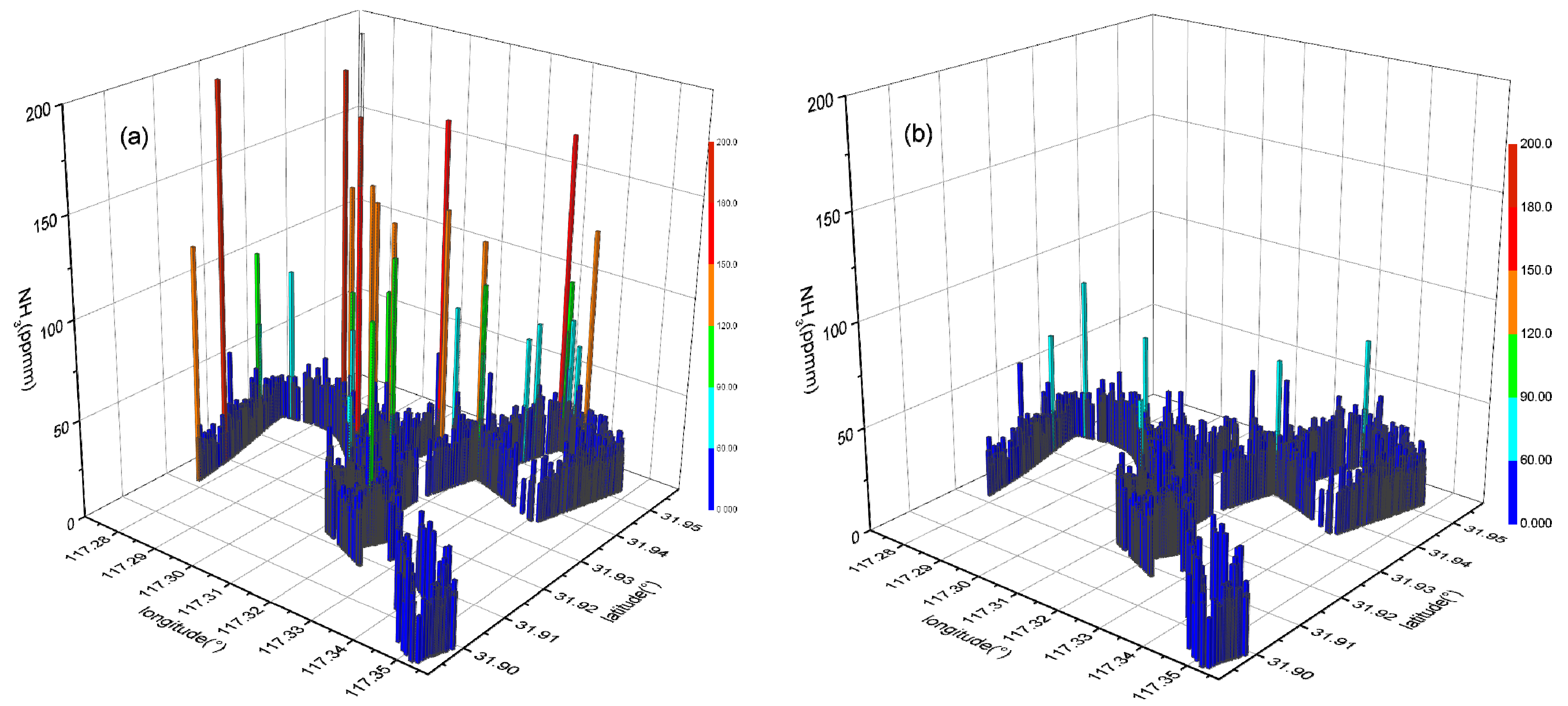
The NH3 column concentrations before and after rejection are visualized using a time series and a three-dimensional distribution diagram (Figure 11). The monitoring results include the latitude, longitude, and NH3 column concentration, and the gas concentration is represented by the small colored columns. From the mobile monitoring results, we can see that the average column concentration of NH3 before the rejection of the abnormal spectra was 30.221 ppmm, and, after the rejection of the anomalous spectra via the spectral data preprocessing method proposed in this paper, the average column concentration of NH3 was 26.648 ppmm.

Figure 11.
Mobile monitoring results. (a) Stereograms of pre-rejection NH3 concentrations and (b) stereograms of post-rejection NH3 concentrations.
5. Conclusions
We proposed a spectral rejection method for preprocessing data from vehicle-mounted Fourier transform spectrometers for occultation fluxes. This method introduces a neural network system, does not require the preparation of training spectra or the setting of fixed correlation comparison coefficients, and has automatic advantages in updating weights. Taking the column concentration measurement of NH3 as an example, we analyzed 1739 experimentally measured spectra in the range of 915 cm−1~980 cm−1 and used the least squares method to fit the transmission spectra. The average RMS of the rejected spectral fit residuals was 4.28% and that of the effective spectral fit residuals was 0.95%. The experimental results show that the improved spectral data preprocessing method proposed in this paper can be used to process the spectral data from a vehicle-mounted occultation flux–Fourier transform spectrometer, which greatly improves the detection rate of abnormal spectra and reduces the impact of abnormal spectra on gas concentration calculations. To store more effective data, the next step will be to improve the tracking accuracy and speed of the solar tracking system and the stability of the spectrometer under vehicular motion.
Author Contributions
Conceptualization, Y.D. and L.X.; Formal analysis, Y.D. and L.X.; Funding acquisition, L.J. and Y.S.; Investigation, L.X.; Methodology, Y.D.; Resources, J.L. and W.L.; Software, Y.D., S.S., Y.S. and L.X.; Validation, S.S.; Writing—original draft, Y.D.; Writing—review & editing, Y.D. and L.X. All authors have read and agreed to the published version of the manuscript.
Funding
Project supported by the key R&D program of Anhui Province, grant number 2022m07020009, the National Natural Science Foundation of China, grant number 52027804 and the Special Funds of the National Natural Science Foundation of China, grant number 41941011.
Institutional Review Board Statement
Not applicable.
Informed Consent Statement
Not applicable.
Data Availability Statement
The data underlying the results presented in this paper are not publicly available at this time, but may be obtained from the authors upon reasonable request.
Conflicts of Interest
The authors declare no conflicts of interest.
References
- Sussmann, R.; Stremme, W.; Buchwitz, M.; De Beek, R. Validation of ENVISAT/SCIAMACHY columnar methane by solar FTIR spectrometry at the Ground-Truthing Station Zugspize. Atmos. Chem. Phys. Discuss 2005, 5, 2419–2429. [Google Scholar] [CrossRef]
- Mellqvist, J.; Samuelsson, J.; Johansson, J.; Rivera, C.; Lefer, B.; Alvarez, S.; Jolly, J. Measurements of industrial emissions of alkenes in Texas using the solar occultation flux method. J. Geophys. Res. 2010, 115, D00F17. [Google Scholar] [CrossRef]
- Baidar, S.; Kille, N.; Ortega, I.; Sinreich, R.; Thomson, D.; Hannigan, J.; Volkamer, R. Development of a digital mobile sun tracker. Atmos. Meas. Tech. 2016, 9, 963–972. [Google Scholar] [CrossRef]
- Washenfelder, R.A.; Toon, G.C.; Blavier, J.-F.; Yang, Z.; Allen, N.T.; Wennberg, P.O.; Vay, S.A.; Matross, D.M.; Daube, B.C. Carbon dioxide column abundances at the Wisconsin Tall Tower site. J. Geophys. Res. Atmos. 2006, 111, 22305. [Google Scholar] [CrossRef]
- Connor, B.J.; Sherlock, V.; Toon, G.; Wunch, D.; Wennberg, P.O. GFIT2: An experimental algorithm for vertical profile retrieval from near-IR spectra. Atmos. Meas. Tech. 2016, 9, 3513–3525. [Google Scholar] [CrossRef]
- Qu, L.; Liu, J.; Deng, Y.; Xu, L.; Hu, K.; Yang, W.; Jin, L.; Cheng, X. Analysis and Adjustment of Positioning Error of PSD System for Mobile SOF-FTIR. Sensors 2019, 19, 5081. [Google Scholar] [CrossRef] [PubMed]
- Shen, X.; Ye, S.; Xu, L.; Hu, R.; Jin, L.; Xu, H.; Liu, J.; Liu, W. Study on baseline correction methods for the Fourier transform infrared spectrum with different signal-to-noise ratios. Appl. Opt. 2018, 57, 5794–5799. [Google Scholar] [CrossRef] [PubMed]
- Shao, L.; Pollard, M.J.; Griffiths, P.R.; Westermann, D.T.; Bjorneberg, D.L. Rejection criteria for open-path Fourier transform infrared spectrometry during continuous atmospheric monitoring. Vib. Spectrosc. 2007, 43, 78–85. [Google Scholar] [CrossRef]
- Liu, Z. Study on the Vehicular FTIR-SOF Monitoring Method for Industrial Emission of Harmful Gases. Ph.D. Thesis, Chinese Academy of Sciences, Beijing, China, 2010. [Google Scholar]
- Ahookhosh, M.; Artacho, F.J.A.; Fleming, R.M.T.; Vuong, P.T. Local convergence of the Levenberg-Marquardt method under Holder metric subregularity. Adv. Comput. Math. 2019, 45, 2771–2806. [Google Scholar] [CrossRef]
- Chalup, S.; Maire, F. A study on hill climbing algorithms for neural network training. In Proceedings of the 1999 Congress on Evolutionary Computation-CEC99 (Cat. No. 99TH8406), Washington, DC, USA, 6–9 July 1999; Volume 3, pp. 2014–2021. [Google Scholar] [CrossRef]
- Dimitrov, D.K.; Peixoto, L.L. An Efficient Algorithm for the Classical Least Squares Approximation. SIAM J. Sci. Comput. 2020, 42, A3233–A3249. [Google Scholar] [CrossRef]
- Hammer, C.L.; Small, G.W.; Combs, R.J.; Knapp, R.B.; Kroutil, R.T. Artificial Neural Networks for the Automated Detection of Trichloroethylene by Passive Fourier Transform Infrared Spectrometry. Anal. Chem. 2000, 72, 1680–1689. [Google Scholar] [CrossRef] [PubMed]
- Yuan, S.; Shi, L.; Yao, B.; Li, F.; Du, Y. A Hyperspectrum Anomaly Detection Algorithm Using Sub-Features Grouping and Binary Accumulation. IEEE Geosci. Remote Sens. Lett. 2022, 19, 6007505. [Google Scholar] [CrossRef]
- Ma, K.; Leung, H.; Jalilian, E.; Huang, D. Deep learning on temporal-spectrum data for anomaly detection. In Proceedings of the Ground/Air Multisensor Interoperability, Integration, and Networking for Persistent ISR VIII: 101900D, Anaheim, CA, USA, 4 May 2017. Society of Photo-optical Instrumentation Engineers. International Society for Optics and Photonics. [Google Scholar]
- Kohonen, T. Self-organized formation of topologically correct feature maps. Biol. Cybern. 1982, 43, 59–69. [Google Scholar] [CrossRef]
- Ripalda, J.M.; Buencuerpo, J.; García, I. Solar cell designs by maximizing energy production based on machine learning clustering of spectral variations. Nat. Commun. 2018, 9, 5126. [Google Scholar] [CrossRef] [PubMed]
- Shalaginov, A.; Franke, K. A New Method for an Optimal SOM Size Determination in Neuro-Fuzzy for the Digital Forensics Applications. In Proceedings of the Advances in Computational Intelligence: 13th International Work-Conference on Artificial Neural Networks, IWANN 2015, Palma de Mallorca, Spain, 10–12 June 2015; International Work-Conference on Artificial Neural Networks. Springer: Cham, Switzerland, 2015. [Google Scholar] [CrossRef]
- Xu, L.; Hu, K.; Yang, W.; Qu, L.; Deng, Y.; Jin, L.; Cheng, X. An Automatic Solar Tracking Device and Method on a Mobile Platform. CN201911346126.3, 24 December 2019. (In Chinese). [Google Scholar]


Disclaimer/Publisher’s Note: The statements, opinions and data contained in all publications are solely those of the individual author(s) and contributor(s) and not of MDPI and/or the editor(s). MDPI and/or the editor(s) disclaim responsibility for any injury to people or property resulting from any ideas, methods, instructions or products referred to in the content. |
© 2024 by the authors. Licensee MDPI, Basel, Switzerland. This article is an open access article distributed under the terms and conditions of the Creative Commons Attribution (CC BY) license (https://creativecommons.org/licenses/by/4.0/).