Mathieu–Hill Equation Stability Analysis for Trapped Ions: Anharmonic Corrections for Nonlinear Electrodynamic Traps

Abstract

The stability properties of the Hill equation are discussed, especially those of the Mathieu equation that characterize ion motion in electrodynamic traps. The solutions of the Mathieu-Hill equation for a trapped ion are characterized by employing the Floquet theory and Hill’s method solution, which yields an infinite system of linear and homogeneous equations whose coefficients are recursively determined. Stability is discussed for parameters a and q that are real. Characteristic curves are introduced naturally by the Sturm–Liouville problem for the well-known even and odd Mathieu equations $c{e}_m(z,q)$ and $s{e}_m(z,q)$. In the case of a Paul trap, the stable solution corresponds to a superposition of harmonic motions. The maximum amplitude of stable oscillations for ideal conditions (taken into consideration) is derived. We illustrate the stability diagram for a combined (Paul and Penning) trap and represent the frontiers of the stability domains for both axial and radial motion, where the former is described by the canonical Mathieu equation. Anharmonic corrections for nonlinear Paul traps are discussed within the frame of perturbation theory, while the frontiers of the modified stability domains are determined as a function of the chosen perturbation parameter and we demonstrate they are shifted towards negative values of the a parameter. The applications of the results include but are not restricted to 2D and 3D ion traps used for different applications such as mass spectrometry (including nanoparticles), high resolution atomic spectroscopy and quantum engineering applications, among which we mention optical atomic clocks and quantum frequency metrology.

1. Introduction

Linear differential equations (LDEs) with variable (periodic) coefficients are ubiquitous in both physics and engineering, but their solutions are generally identified by means of numerical simulations. In an effort to identify a solution for such a system, it is essential to infer the so-called Floquet or characteristic exponents that define a fundamental matrix associated to the system [1]. One of the most prevalent approaches used in case of LDEs with periodic coefficients is based on a truncated Fourier series [2] whose coefficients are derived by means of the Harmonic Balance (HB) approximate method [3,4], which is employed to investigate nonlinear oscillating systems described by ordinary nonlinear differential equations (NLDEs) [5].

Mathieu functions of period $\pi$ or $2\pi$, also known as elliptic cylinder functions, were introduced in 1868 by Mathieu [6] together with the so-called modified Mathieu functions [7] in order to characterize the vibrations of an elastic membrane placed in a fixed elliptical hoop [8,9]. As the Mathieu equation does not possess a closed-form analytic solution, its applications are affected by analytical [10] and numerical approximation schemes [11] along with the nonlinear analysis of the associated stability charts [12,13]. Therefore, analytical solutions of Mathieu–Hill (MH) or Duffing equations are generally investigated by means of various perturbation techniques [14,15,16], while other approaches also use non-perturbative techniques to characterize the parametric damping nonlinear Mathieu–Duffing oscillator [17].

Analytic periodic approximations for differential equations of Hill type are investigated in Ref. [3], where two different methods are employed in the straightforward case of a Mathieu equation. The first method is triggered by the HB method [4,18], with an aim to identify analytic approximations for the critical values and focus on periodic solutions of the Mathieu equation. It is demonstrated that these kinds of solutions are valid for any values of the parameter q. The second method exploits truncations of the Fourier series [2].

In the last decades, Mathieu-type linear or nonlinear parametric differential equations have been the subject of large scientific interest because of their frequent use in applied mathematics [19,20], quantum physics [21,22], quantum optics [23], engineering [12], analytical chemistry and mechanics [13,14], along with general relativity [24] and astrophysics [25].

The advent of ion traps (ITs) has produced remarkable breakthroughs in modern physics, as they enable the trapping of electrically charged particles—usually in ultra-high vacuum (UHV)—which creates an almost interaction-free environment [26,27,28,29,30] that delivers long coherence times and narrow atomic lines. The particles are localized in a sharply defined region in space under conditions of dynamical equilibrium [31,32]. Hence, an IT is a versatile tool to perform high-resolution atomic spectroscopy. Ion dynamics in a Paul (or RF) trap [26,33] is characterized by a MH-type equation [21,34]. The Paul trap apparatus [in the case of both 2D linear ion traps (LITs) and 3D versions] has been developed and refined for high-finesse quantum engineering experiments, high-precision spectroscopy [35,36], classical mass spectrometry (MS) [37,38,39,40,41,42] and chemical analysis [43], including the detection of aerosols and chemical warfare [44,45,46,47,48,49,50,51,52].

Apart from that, ITs also enable exceptional control in preparing and manipulating atomic quantum states [53,54,55,56,57,58] because they make possible applications such as quantum logic [59,60,61,62,63], quantum sensing [64,65,66,67], quantum metrology [68,69] and even time fractals [70] or time crystals [71]. To these, one adds high-accuracy optical frequency standards [72,73,74,75], which are amongst the most sensitive quantum sensors [76,77] used to perform searches for physics beyond the Standard Model (BSM) [78,79,80] or to disseminate atomic time scales and redefine the SI unit of time, the second [81,82,83,84,85]. The sensitivity of optical atomic clocks [72,86] is limited by the Standard Quantum Limit (SQL) imposed by the inherent projection noise of a quantum measurement [87]. Recent developments in atomic physics have enabled quantum engineering of many-body entangled states that boost the performance of quantum sensors beyond the SQL [55,66,88,89]. Furthermore, it is anticipated that use of compound atomic clocks can enhance the stability of single ion clocks with long clock transition lifetimes to levels comparable to those of optical lattice clocks [75,90]. For ion species characterized by shorter lifetimes, the stability can be improved directly by increasing the number of ions. Nevertheless, this approach requires special care in the selection of the atomic transition and offers the potential for a stability beyond the SQL, which could represent a viable approach to further improve the stability of optical clocks [91] and provide quantum-limited optical time transfer [82,92], with an aim to achieve intercontinental clock comparisons through a common-view node in geostationary orbit (GEO). Several missions such as NASA’s Deep Space Atomic Clock (DSAC) or the Atomic Clock Ensemble in Space (ACES), along with ongoing or future European Space Agency (ESA) missions are based on deploying optical clocks in space.

An electrodynamic (Paul) trap is highly susceptible to geometric imperfections and electrode misalignment [39,93,94], which results in the occurrence of local minima in the trapping electric potential and nonlinear resonances in ion dynamics [42,95,96,97,98]. In the case of 2D traps, motional coupling between axial and radial directions is reported [99,100]. Trap potential deviations with respect to an ideal quadrupole lead to parasitic effects [101] which impose limitations in an explicit manner on the number of ions that can be confined, and implicitly on the signal to noise ratio (SNR) [65,102,103]. The effects produced by higher-order anharmonic terms [60] in the electric trapping potential (for linear strings of trapped ions) is investigated in [104]. As the ratio between the anharmonic and harmonic terms typically increases when the ion–electrode distance is reduced, it is demonstrated that anharmonic effects become more critical by lessening the ion trap scale. This requires special care, particularly in the case of single-ion [90,105,106] and multi-ion optical clocks [74,91,107,108] or in quantum sensing [109] and quantum computing experiments with trapped ions [65,110]. On the other hand, it is demonstrated that an increased dodecapole potential generated in an asymmetric LIT [99] opens new pathways for exciting applications in mass spectrometry or Coulomb crystals. Such a setup also enables dark ion (inappropriate confined species) elimination from a trapped ion chain consisting of physical qubits [42], or performing searches for time and parity violations that could constrain sources of new physics BSM [78,111,112].

The solution of a weakly nonlinear Mathieu equation (NME) is employed in [113] to characterize ion dynamics in the neighborhood of the stability boundary of ideal ITs (for which higher-order terms of the trap electric potential are discarded). The HB method [4] is employed in [114] to explore the coupling effects of hexapole and octopole fields on ion dynamics in a quadrupole ion trap (QIT). Ion motion characteristics, e.g., motion center displacement, secular frequency shift, nonlinear resonance curve and buffer gas damping effects have been investigated. It turns out that hexapole fields have a larger impact on ion motion center displacement, while octopole fields are mainly responsible for the ion secular frequency shift. In addition, the nonlinear features induced by hexapole and octopole fields may enhance or cancel each other. Ion dynamics in nonlinear Paul traps is investigated in [115] using the theoretical HB method, which allows one to derive the analytical ion trajectory and ion motion frequency in the superimposed octopole field by solving the NME [101]. The HB method is then validated by means of the numerical fourth-order Runge–Kutta (4th RK) method.

Amongst other issues, the response of a Duffing oscillator (DO) [15,116] to a harmonic excitation, in presence of (viscous) damping, is known to exhibit hysteretic and chaotic behaviors [1,13,100,117,118]. It is demonstrated that in particular cases, the damping force may induce instability in the ion dynamics [119,120]. For instance, Ref. [121] explores the role of field inhomogeneities in altering the stability boundaries in nonlinear Paul traps, taking into account higher-order terms in the equation of motion. The Poincaré–Lighthill–Kuo (PLK) method is employed in [122] to derive an analytical expression on the stability boundary and characterize the ion trajectory within a nonlinear Paul trap. The paper shows that a multipole superposition model (which essentially involves the octopole component) explains quite well how the field inhomogeneities shift the stable trapping region.

Particle dynamics in a nonlinear quadrupole Paul trap with octopole anharmonicity (which is a well-known dissipative system [32,123]) is described by an NME [4,124], which includes all perturbing contributions such as damping, multipole terms of the potential and a harmonic excitation force (periodic kicking). To complicate the picture even more, the ion also undergoes interaction with a laser field [125], in presence of contributions from the hexapole and octopole fields that superpose over the harmonic trap potential. Hence, it was demonstrated that a damped parametric oscillator (PO) levitated in a Paul trap exhibits fractal properties and complex chaotic orbits, along with the emergence of strange attractors (which are often called fractal sets) [125,126]. Ion motion on the strange attractor exhibits sensible dependence on the initial conditions. Several recent papers also demonstrate that ion dynamics in a Paul trap can be assimilated with the equation that describes a damped driven DO [100,101]. The equation of motion for such system is similar to a perturbed Duffing-type equation [15], which is a generalization of the linear differential equation that describes damped and forced harmonic motion [127,128].

Ref. [129] explores classical and quantum integrability for a trapped ion Hamiltonian in 3D space, under conditions of a non-quadratic potential with superpositions of the hexapole and octopole terms in the series expansion of the electric potential [130]. The Painlevé analysis is employed to determine new integrable cases. It is also demonstrated that the 3D perturbed Hamiltonian is completely integrable in the sense of Liouville [129]. Recent results also show the effective potential of an ion in 3D multipole fields in the mixed-mode is characterized by multiple isolated local minima. In addition, the specific number and spatial positions of the stable quasi-equilibrium points depend on the $a/q$ parameters ratio and the polarity of the electrodes’ DC voltage component [131]. An iterative method is employed to derive the stability parameters from measured secular frequencies, which is presented in Ref. [105].

Structure of the Paper

Section 1 is a review of ion traps and their deep impact for modern physics and quantum technologies. Section 2 and Section 3 investigate the properties of the Mathieu–Hill (MH) equations based on Floquet’s theorem, Hill’s Method solution and Sträng’s technique [132]. We demonstrate how the recurrence relationship that supplies the Floquet exponent is derived. The stability properties of the solutions of the MH equation for a trapped ion are discussed for real parameters a and q. The issue of bounded or unbounded ion dynamics is also discussed, pointing out that the $(a,q)$ plan is divided into stability and instability regions. A stable solution of motion corresponds to a superposition of harmonic motions and we find the frequency spectrum in such case. The stability diagram for an electrodynamic (Paul) trap is illustrated as a function of the Mathieu function eigenvalues. We also illustrate the stability diagram for a combined trap, where both axial and radial dynamics are considered, and we investigate the damped PO which generally exhibits fractal properties, chaotic complex orbits and exotic attractors [125,126,133]. Ion trajectories in the phase space are explored and we infer the transfer matrix along with the maximum amplitude of stable oscillations for ions confined in a quadrupole Paul trap.

We demonstrate that in case of small values of the trap operating parameters $(a,q)$, located within the first stability region, higher harmonics are practically insignificant and the fundamental frequency prevails. We identify the solution of the MH equation in such a case and we further apply the pseudopotential method to infer the shift in the solution, along with the first correction.

Section 4 approaches an issue of large interest by investigating multipole anharmonicities of the trap electric potential. We employ the perturbation theory and supply the modified frontiers of the stability diagram in case of an electrodynamic trap with a nonlinear octopole term of the electric potential, as a function of the perturbation parameter we choose. Annexes are intended to help the reader acquire a better grasp of the mathematics involved, including the perturbation theory technique, with a focus on simplicity.

2. Mathieu–Hill Equations

The Hill differential equation is similar to Mathieu’s equation but exhibits a more general nature. It arises in Hill’s method [134,135] to establish the motion of the Lunar Perigee and it represents a generalization of the Mathieu equation [19,136,137]. The MH equation is a homogeneous, second-order ordinary differential equation (ODE), with variable (periodic) coefficients [4,13]. It characterizes dynamical systems that exhibit intrinsic periodicity and parametric behaviour, such as the modulation of radio carrier waves, transverse vibrations of a tense elastic membrane, the stability of periodic motion in a nonlinear system, as well as the focus and defocus of beams in particle accelerators [138,139], and it is also employed to explore planetary dynamics [25]. The Hill equation takes the canonical or standard form of a reduced linear equation of the second order [8,10,20,140]:

$$\frac{d^{2}w}{d{\tau }^2}+J\left(\tau \right)w=0$$

(1)

where J stands for a continuous and even function that is periodic in $\tau$. The period is usually taken equal to $\pi$ for historical reasons [140]. The differential Equation (1) was discussed by Mathieu in 1868 in connection with the problem of vibrations of an elliptic membrane [6]. It is also assumed that the function $J\left(\tau \right)$ can be expressed as a Fourier series [137]

$$J\left(\tau \right)={\theta }_0+\sum _{s=1}^{\infty }2{\theta }_{s}cos2\tau$$

(2)

which converges within an infinite band in the $\tau$ plan that includes the real axis. If ${\theta }_s=0$ for $s\ge 2$, then Equation (1) turns into the Mathieu equation. Furthermore, Equation (1) can also be arranged as follows:

$$\frac{d^{2}w}{d{\tau }^2}+\left[a-2q\psi \left(\tau \right)\right]w=0$$

(3)

where $\psi \left(\tau \right)$ represents a continuous and even function of period $\pi$, while a and q denote adimensional parameters [141]. The parameter a is often called the characteristic value or eigenvalue, and it is generally determined by means of given boundary conditions, while the $-2q$ parameter represents a fixed datum. The solution $w\left(\tau \right)$ for a given value of a is usually called the eigenfunction. As a rule, one seeks out periodic solutions of Equation (3) with boundary conditions defined at two finite fixed points, for example, 0 and p, provided in the form $w\left(0\right)=w\left(p\right)$ and $\dot{w}\left(0\right)=\dot{w}\left(p\right)$, where p is the period. This represents a particular case of a Sturm–Liouville problem [3,141]. In the particular case of Mathieu’s general equation or Hill’s equation, a fundamental system of solutions consists of $e^{\mu \tau }\varphi \left(\tau \right)$ and $e^{-\mu \tau }\varphi \left(-\tau \right)$, as the equation is invariable to the change $-\tau \to \tau$. Consequently, Floquet demonstrated that the complete solution of Mathieu’s general Equation (1) can be expressed as follows [136,137,140,142,143]:

$$w=A{e}^{\mu \tau }\varphi \left(\tau \right)+B{e}^{-\mu \tau }\varphi \left(-\tau \right)$$

(4)

where $\mu \in \mathbb{C}$ is called the Floquet or characteristic exponent and it is a definite function of the a and q parameters, $\varphi$ denotes a periodic class $C^2$ function (twice continuously differentiable) [144], while A and B stand for arbitrary constants. Then, based on the Floquet’s theorem and according to Hill’s method one may assume a series solution:

$$w=e^{\mu \tau }\sum _{s=-\infty }^{\infty }{c}_{2s}{e}^{2is\tau }=\sum _{s=-\infty }^{\infty }{c}_{2s}{e}^{\left(\mu +2is\right)\tau }$$

(5)

By introducing Equation (5) into Equation (1), one infers a recurrence relation:

$${\left(\mu +2is\right)}^2{c}_{2s}+\sum _{m=-\infty }^{\infty }{\theta }_{2m}{c}_{2s+m}=0,s\in \mathbb{Z},$$

(6)

where $\mathbb{Z}$ is the set of integer numbers, with ${\theta }_{-2m}={\theta }_{2m}$. If one tries to eliminate the term $c_{2s}$ in Equation (6), then a non-convergent infinite determinant [137] would result. To avoid such an outcome, every expression in Equation (6) is divided to its central term ${\left(\mu +2is\right)}^2+{\theta }_0$. To determine the characteristic exponent, one multiplies the system matrix described by Equation (6) with a diagonal matrix. Then, a matrix results whose diagonal entries are each equal to unity, assuming that none of the terms ${\left(\mu +2is\right)}^2+{\theta }_0$ vanish. By denoting the determinant of this matrix as $▵\left(i\mu \right)$, the equation that determines the Floquet exponent $\mu$ is [137]

$$▵\left(i\mu \right)=0$$

(7)

Then, Equation (7) can be further arranged as

$$cosh\pi \mu =1-2▵\left(0\right){sin}^2\frac{1}{2}\pi {\sqrt{\theta }}_0$$

(8)

When $\mu$ has been determined, the $c_{2s}$ coefficients can be inferred in terms of $c_0$ and co-factors of $▵\left(i\mu \right)=0$. Thus, the solution of the Hill differential equation is complete. In the case of a fairly rapid convergence of the determinant $▵\left(i\mu \right)$, Equation (7) can be used in its algebraic as well as recursive and explicit form, which represents Hill’s original method [9,137]. The evaluation of the determinant $▵\left(0\right)$ and the use of Equation (8) represents an alternative method when this determinant converges quite well. A practical method to solve the Hill equation was suggested by Brillouin [140] based on the expression

$${sinh}^2\left(\frac{1}{2}\pi \mu \right)={\dot{w}}_1\left(\frac{\pi }{2}\right)w_2\left(\frac{\pi }{2}\right)$$

(9)

where $w_1$ and $w_2$ stand for two fundamental solutions, and ${\dot{w}}_1$ stands for the time derivative. If a periodic fundamental solution exists for the Mathieu equation, then the existence of the other fundamental solution is forbidden and the characteristic exponent of the periodic solution corresponds to the a and q parameters of the characteristic curves that separate the stability domains. In the case of the Hill equation, such a property is not generally satisfied. Equation (9) is useful to compare with Whittaker’s theory on the Hill equation [137]. The advantage of applying such method lies in the fact that it works with periodic $J\left(\tau \right)$ functions that exhibit a finite number of discontinuities.

For example, Ref. [145] investigates the modes which diagonalize the dynamical problem for linearly coupled Mathieu equations, which leads to the Floquet–Lyapunov transformation, where the motion is associated with decoupled linear oscillators. The method is then used to solve the Heisenberg equations of the corresponding quantum–mechanical problem and to determine the quantum wavefunctions for stable oscillations in the configuration (Hilbert) space. Such a transformation and solution can be applied to more generic linear systems with periodic coefficients, such as coupled Hill equations and periodically driven parametric oscillators.

3. Stability of the Solutions of the Mathieu–Hill Equation for a Trapped Ion

The equation of motion for an ion confined within a Paul (electrodynamic) trap exhibits the standard form of the Mathieu equation [19,146,147,148]:

$$\frac{d^{2}w}{d{\tau }^2}+\left[a-2qcos\left(2\tau \right)\right]w=0$$

(10)

with $\tau =\Omega t/2$ being dimensionless, where $\Omega$ is the RF of the trapping voltage $V_0$ applied between the electrodes. We introduce

$$\left\{\begin{array}{cc}{a}_z=-2a_x=-2a_y=-\frac{8Q{U}_0}{m{\Omega }^2\left(r_0^2+2z_0^2\right)}\hfill & \\ q_z=-2q_x=-2q_y=\frac{4Q{V}_0}{m{\Omega }^2\left(r_0^2+2z_0^2\right)}\hfill & \hfill \end{array}\right.$$

(11)

where Q is the ion electric charge, m denotes the ion mass, $r^2=r_0^2+2z_0^2$ with $r_o$ and $z_0$ being the trap semiaxes, and $U_0$ stands for the DC trapping voltage applied to the trap (endcap) electrodes. In addition, $a_x=-a_y$ and $q_x=-q_y$. To investigate the stability of ion trajectories, one uses the stability properties of the Mathieu equation solutions. As shown in Equations (4) and (5), the solution of Equation (10) can be expressed as a Hill series

$$w\left(\tau \right)=A{e}^{\mu \tau }\sum _{s=-\infty }^{\infty }{c}_{2s}{e}^{2is\tau }+B{e}^{-\mu \tau }\sum _{s=-\infty }^{\infty }{c}_{2s}{e}^{-2is\tau }$$

(12)

where the A and B constants are determined from the initial conditions. If $i\mu \notin \mathbb{Z}$, then using Equation (12), one infers a fundamental system of solutions associated to Equation (10) for $A=1,B=0$ and $A=0,B=1$ (the Floquet theorem [19,137]). The characteristic exponent $\mu$ and the $c_{2s}$ coefficients are functions of the parameters a and q [146].

By introducing the solution supplied by Equation (5) in the Mathieu Equation (10), the latter is cast into

$$\sum _{s=-\infty }^{\infty }{c}_{2s}\left[{\left(\mu +2is\right)}^2+a-2q\frac{e^{2i\tau }+e^{-2i\tau }}{2}\right]e^{\left(\mu +2is\right)\tau }=0$$

(13)

which, after matching the terms according to the powers of s, results in a recurrence relation

$$-q{c}_{2s-2}+\left[{\left(\mu +2is\right)}^2+a\right]-q{c}_{2s+2}=0$$

(14)

Further on, one multiplies with $i^2=-1$ and then divides by the middle term in Equation (14), which leads to an infinite system of linear equations which are homogeneous in the $c_{2s}$ coefficients [142]:

$$\frac{q}{{\left(2s-\mu i\right)}^2-a}{c}_{2s-2}+c_{2s}+\frac{q}{{\left(2s-\mu i\right)}^2-a}{c}_{2s+2}=0$$

(15)

which can be expressed as

$${\gamma }_{2s}{c}_{2s-2}+c_{2s}+{\gamma }_{2s}{c}_{2s+2}=0,s=0,\pm 1,\pm 2,\dots$$

(16)

with

$${\gamma }_{2s}=q{\left[{\left(2s-i\mu \right)}^2-a\right]}^{-1}$$

(17)

The system of Equation (16) admits a nontrivial solution if and only if the corresponding infinite determinant $▵\left(i\mu \right)$ vanishes for s noninfinite [137,149]

$$△\left(i\mu \right)=\left|\begin{array}{ccccc}\dots & & & & \\ & {\gamma }_{-2}& 1& {\gamma }_{-2}& & \\ & & {\gamma }_0& 1& {\gamma }_0& \\ & & & {\gamma }_2& 1& {\gamma }_2\\ & & & & & \dots \end{array}\right|$$

(18)

Due to the symmetry of $△\left(0\right)$, ${\gamma }_{-j}={\gamma }_j$. Solving this determinant is not a simple issue, which is why one uses the approach of Whittaker [137]. The method is described in Appendix A and it was introduced by Sträng [132,149]. The equation

$$▵\left(\mu \right)=0$$

(19)

supplies the characteristic exponent $\mu$, while Equation (16) enable one to recursively determine the coefficients $c_{2s}$. The infinite-order determinant $▵\left(\mu \right)$ is absolutely convergent and it represents a meromorphic function [150,151] of $\mu$, with simple poles for $\mu =\pm i\left(\sqrt{a}+2s\right);s=0,\pm 1,\dots$. Hence, Equation (18) is equivalent to [19]

$$cosh\left(\pi \mu \right)=1+2▵\left(0\right){\left[sin\left(\pi \sqrt{a}/2\right)\right]}^2$$

(20)

Hereinafter, we discuss the stability of the solutions of Equation (10) for $\tau ,a,q\in \mathbb{R}$. The solution of Equation (12) is stable or unstable if $\left|w\left(\tau \right)\right|$ is bounded or unbounded along the $\tau >0$ semi-axis, respectively. From Equation (20), one infers $cosh\left(\pi \mu \right)\in \mathbb{R}$ which renders the solution of Equation (12) as stable when $\left|cosh\left(\pi \mu \right)\right|<1$, in other words when $i\mu$ is a real non-integer. If $\left|cosh\left(\pi \mu \right)\right|>1$ then $\alpha =\Re e\mu \ne 0$, while $\left|w\left(\tau \right)\right|$ is bounded along the $\tau$ axis. In such a case, $\left|w\left(\tau \right)\right|$ is bounded along the $\tau >0$ semiaxis only when $A=0,\alpha >0$ or $B=0,\alpha <0$. As an outcome, the $\left(a,q\right)$ plan is divided into stability regions with $\left|cosh\left(\pi \mu \right)\right|<1$ and instability regions characterized by $\left|cosh\left(\pi \mu \right)\right|>1$, separated by the curve $\left|cosh\left(\pi \mu \right)\right|=1$ for which a stable and periodic solution of Equation (10) exists, although the general solution is unbounded. The curves characterized by integer values of $i\mu$ are called characteristic curves. They are naturally introduced by means of the Sturm–Liouville (eigenvalue) problem [137,141,152] for the Mathieu functions $c{e}_m\left(z,q\right)$ and $s{e}_m\left(z,q\right)$ [20,148], which are treated as characteristic functions of Equation (10) with the limit conditions

$$\frac{dw\left(0\right)}{d\tau }=\frac{dw\left(\pi \right)}{d\tau }=0,w\left(0\right)=w\left(\pi \right)=0$$

(21)

The $c{e}_m\left(z,q\right)$ and $s{e}_m\left(z,q\right)$ functions [7,153] are even and odd, respectively, known up to a constant factor, with period $\pi$ when m is even and with period $2\pi$ when m is odd [19,137]. The characteristic curves $a_m\left(q\right)$ and $b_m\left(q\right)$ correspond to the Mathieu functions $c{e}_m\left(z,q\right)$ with $m=0,1,\dots$ and $s{e}_m\left(z,q\right)$ with $m=1,\dots$, respectively. In addition, the characteristic curves are analytical in q, while being characterized by the subsequent properties [137]:

$$a_{2m}\left(q\right)=a_{2m}\left(-q\right),b_{2m+2}\left(q\right)=b_{2m+2}\left(-q\right),a_{2m+1}\left(q\right)=a_{2m+1}\left(-q\right)$$

(22)

$$a_{2m+1}\left(-q\right)=b_{2m+1}\left(q\right),a_m\left(q\right)<b_{m+1}\left(q\right)<a_{m+1}\left(q\right)$$

(23)

with $m=0,1,\dots$ and $q>0$.

The family of curves characterized by $\left|cosh\left(\pi \mu \right)\right|=1$ coincides with the family made up by the characteristic curves $a_m\left(q\right)$ with $m=0,1,\dots$ and $b_m\left(q\right)$ with $m=1,\dots$, which divide the $\left(a,q\right)$ plan into stability regions [ranging from $a_m\left(q\right)$ to $b_{m+1}\left(q\right)$ for $q\ge 0$ and from $a_m\left(q\right)$ to $a_{m+1}\left(q\right)$ or from $b_m\left(q\right)$ to $b_{m+1}\left(q\right)$ for $q\le 0$] and instability regions located below $a_0\left(q\right)$ or ranging from $b_m\left(q\right)$ to $a_m\left(q\right)$.

Ref. [154] shows that in case of microparticles levitated within a 2D linear Paul trap (LPT) operating under standard temperature and pressure (STP) conditions (in air), the Mathieu equations describing the trapping process are homogeneous along the x and y axes, with the well-known solutions and stability domains. On the other hand, the z axis motion is described by an inhomogeneous Mathieu equation. In this case, stability is obtained for (a) $i\mu \in \mathbb{R}$, (b) $\mu \in \mathbb{R}$ and $\mu <\Lambda$ and (c) $\mu -i\in \mathbb{R}$ and $|\mu -i|<\Lambda$, where $\mu$ is the Floquet exponent, $\Lambda =K/m\Omega$, K stands for the coefficient which describes the drag aerodynamic force and m represents the particle mass. Hence, stability regions for solutions of the inhomogeneous equations of motion in the presence of drag forces include both the stability regions of the homogeneous equations along with a part of the instability regions, which extends them considerably.

The Mathieu Equation (10) exhibits $\pi -$ and $2\pi -$ periodic solutions on continuous stability curves $a=a\left(q\right)$, starting from points $a=n^2,n=1,2,3,\dots$ Furthermore, the periodic solutions and the boundaries between stability and instability regions in the $(a,q)$ parameter plane can be found by means of the Lindstedt–Poincaré method [16]. A cosine elliptic $c{e}_n$ and a sine elliptic $s{e}_n$ function are associated to any value of n, where each one of these functions has its own characteristic number $a_{c{e}_n}$ and $a_{s{e}_n}$. The Mathieu functions and their eigenvalues (characteristic numbers) in the power series of q for $a,\left|q\right|\ll 1\left(q\simeq 0\right)$ are expressed as follows:

$$a_0\left(q\right)=a_{c{e}_0}\left(q\right)=-\frac{q^2}{2}+\frac{7q^4}{128}-\frac{29q^6}{2304}+\frac{68687q^8}{18874368}+\frac{123707q^{10}}{104857600}+\dots$$

(24)

$$\begin{array}{c}{a}_1\left(q\right)=a_{s{e}_1}\left(q\right)=1+q-\frac{q^2}{8}-\frac{q^3}{64}-\frac{q^4}{1536}+\frac{11q^5}{36864}+\frac{49q^6}{589824}\hfill \\ \hspace{1em}\hspace{1em}\hspace{1em}\hspace{1em}\hspace{1em}\hspace{1em}\hspace{1em}\hspace{1em}\hspace{1em}\hspace{1em}\hspace{1em}+\frac{55q^7}{9437184}-\frac{83q^8}{35389440}-\frac{12121q^9}{15099494400}+\dots \hfill \end{array}$$

(25)

$$\begin{array}{c}{b}_1\left(q\right)=a_{c{e}_1}\left(q\right)=1-q-\frac{q^2}{8}+\frac{q^3}{64}-\frac{q^4}{1536}-\frac{11q^5}{36864}+\frac{49q^6}{589824}\hfill \\ \hspace{1em}\hspace{1em}\hspace{1em}\hspace{1em}\hspace{1em}\hspace{1em}\hspace{1em}\hspace{1em}\hspace{1em}\hspace{1em}\hspace{1em}-\frac{55q^7}{9437184}-\frac{83q^8}{35389440}+\frac{12121q^9}{15099494400}+\dots \hfill \end{array}$$

(26)

$$a_2\left(q\right)=a_{s{e}_2}\left(q\right)=4+\frac{5q^2}{12}-\frac{763q^4}{13824}+\frac{1002401q^6}{79626240}-\frac{1669068401q^8}{458647142400}+\dots$$

(27)

$$b_2\left(q\right)=a_{c{e}_2}\left(q\right)=4-\frac{q^2}{12}+\frac{5q^4}{13824}-\frac{289q^6}{79626240}+\frac{21391q^8}{458647142400}+\dots$$

(28)

The eigenvalue associated with the even solutions of the Mathieu functions, $c{e}_k(z,q)$, is labelled by $a_k\left(q\right),k=0,1,2,\dots$, while the one associated with the odd Mathieu function, $s{e}_k(z,q)$, is denoted as $b_k\left(q\right),k=1,2,\dots$, as illutrated in Figure 1. The higher rank terms that describe the frontiers of the stability regions are given in Appendix B. A method to generate stability plots for the Mathieu equation in the case of a toroidal ion trap mass analyzer is presented in Ref. [155].

To graphically illustrate the stability diagram (associated to the Mathieu equation) that characterizes the dynamics of an ion confined within a combined quadrupole trap (a combination between a Penning and a Paul trap), we have used Equations (24)–(28) and Equations (A20)–(A28). The result is shown in Figure 2.

In case of a quadrupole Paul trap, the stable solution of the equation of motion (10) (for $\mu =i\beta ,\beta \in \mathbb{R}$) corresponds to a superposition of harmonic motions [21,29,103]

$$w\left(t\right)={\alpha }_1\sum _{s=-\infty }^{\infty }{c}_{2s}cos\left[\left(s+\frac{\beta }{2}\right)\Omega t\right]+{\alpha }_2\sum _{s=-\infty }^{\infty }{c}_{2s}sin\left[\left(s+\frac{\beta }{2}\right)\Omega t\right]$$

(29)

with the frequency spectrum

$${\nu }_s=\left(2s\pm \beta \right)\frac{\Omega }{4\pi },s=0,1,\dots$$

(30)

In Figure 3, we have illustrated the stability diagram for a combined (Paul and Penning) trap. One notices that $a_0,b_1,a_1,b_2,a_2$ represent the frontiers of the stability diagram associated with the canonical Mathieu equation that describes axial motion. We also introduce

$$\begin{array}{c}{c}_0\left(q\right)=c-a_0\left(-q/2\right)/2=c+\frac{1}{16}{q}^2-\frac{7}{4096}{q}^4+\frac{29}{2304}\frac{q^6}{64}\hfill \\ \hspace{1em}\hspace{1em}\hspace{1em}\hspace{1em}\hspace{1em}\hspace{1em}\hspace{1em}\hspace{1em}\hspace{1em}\hspace{1em}\hspace{1em}\hspace{1em}\hspace{1em}-\frac{68687}{18874368}\frac{q^8}{512}-\frac{123707}{104857600}\frac{q^{10}}{2048}\hfill \end{array}$$

(31)

$$\begin{array}{c}{c}_1\left(q\right)=c-a_1\left(-q/2\right)/2=c-\frac{1}{2}+\frac{q}{4}+\frac{q^2}{64}-\frac{q^3}{512}+\frac{1}{1536}\frac{q^4}{32}+\frac{11}{36864}\frac{q^5}{64}\hfill \\ \hspace{1em}\hspace{1em}\hspace{1em}\hspace{1em}\hspace{1em}\hspace{1em}-\frac{49}{589824}\frac{q^6}{128}+\frac{55}{9437184}\frac{q^7}{256}+\frac{83}{35389440}\frac{q^8}{512}-\frac{12121}{15099494400}\frac{q^9}{1024}\hfill \end{array}$$

(32)

$$\begin{array}{c}{d}_1\left(q\right)=c-b_1\left(-q/2\right)/2=c-\frac{1}{2}-\frac{q}{4}+\frac{q^2}{64}+\frac{q^3}{1024}+\frac{1}{1536}\frac{q^4}{32}-\frac{11}{36864}\frac{q^5}{64}\hfill \\ \hspace{1em}\hspace{1em}\hspace{1em}\hspace{1em}\hspace{1em}\hspace{1em}-\frac{49}{589824}\frac{q^6}{128}-\frac{55}{9437184}\frac{q^7}{256}+\frac{83}{35389440}\frac{q^8}{512}+\frac{12121}{15099494400}\frac{q^9}{1024}\hfill \end{array}$$

(33)

Further on, we consider trap operating points of $\left(a,q\right)$ that lie within the first stability region, with $0<\beta <1$ and $q\ge 0$. By minimizing the parameters a and $q\left(a/q\ll 1,q<0.4\right)$, the coefficients $c_{2s}$ (with $s\ne 0$) rapidly converge to zero, in such a way that higher harmonics are practically insignificant and the fundamental frequency ${\nu }_0=\beta \Omega /\left(4\pi \right)$ prevails [156]. In such an event, $w\left(t\right)=w_0\left(t\right)+w_1\left(t\right)$, where $w_0\left(t\right)$ stands for the average of the $w\left(t\right)$ shift during the interval $\left[t,t+2\pi /\Omega \right]$ where $\left|w_1\left(t\right)\right|\ll \left|w_0\left(t\right)\right|$ and $\left|d{w}_1/dt\right|\gg \left|d{w}_0/dt\right|$. Under such circumstances, the solution of the Mathieu equation can be approximated as the solution of the following equation:

$$\frac{d^{2}w}{d{t}^2}=\frac{{\Omega }^2}{4}\left[-a+q\left(\frac{a}{2}+2\right)cos\Omega t-q^2{cos}^2\Omega t\right]w$$

(34)

By averaging Equation (34) over a period of the RF voltage (which is exactly the case of the pseudopotential approximation, when the electric forces that are time-averaged over an RF period generate a harmonic potential [21,29,157,158]), one derives

$$\frac{d^2{w}_0}{d{t}^2}=-{\beta }^2{w}_0,\beta =\sqrt{a+\frac{q^2}{2}}$$

(35)

The shift $w_0$ in Equation (35) corresponds to the harmonic motion of fundamental frequency ${\nu }_0$, while the correction $w_1$ is determined by the higher harmonics $\left(2-\beta \right)\Omega /4\pi$, $\left(2+\beta \right)\Omega /4\pi ,\dots$ The axial frequencies are twice the radial frequencies, $a_z=-2a_r$ and $q_z=-2q_r$, while the trapped ions describe approximate Lissajoux trajectories when the ratio between the frequencies along the axes is 1:1:2. The initial conditions have no effect whatsoever on the stability of ion trajectories, but they establish their position with respect to the area located between the trap electrodes for every operating point $\left(a,q\right)$ fixed within a stability domain. In this regard, the problem of evaluating the maximum amplitude of stable oscillations under given initial conditions is approached. The maximum admits upper bounds determined by the relative position of the electrodes. For optimum operating parameters, it is mandatory to take into account all axes for whom the equation of motion is of Mathieu type.

One considers the stable solution of Equation (29) expressed as

$$w\left(\tau \right)={\alpha }_1{w}_1\left(\tau \right)+{\alpha }_2{w}_2\left(\tau \right)$$

(36)

with

$$w_1\left(\tau \right)=\sum _{s=-\infty }^{\infty }{c}_{2s}cos\left(2s+\beta \right)\tau ,w_2\left(\tau \right)=\sum _{s=-\infty }^{\infty }{c}_{2s}sin\left(2s+\beta \right)\tau$$

(37)

where both $w_1\left(\tau \right)$ and $w_2\left(\tau \right)$ are differentiable functions. If $w\left(\tau \right)\ne 0$ (which also implies that the coefficients ${\alpha }_1,{\alpha }_2\ne 0$) then $w_1$ and $w_2$ are linearly dependent functions. Hence, $w_1$ and $w_2$ form a fundamental system of solutions of the Mathieu equation (10) and the Wronskian determinant [7] is

$$W=w_1\left(\tau \right){\dot{w}}_2\left(\tau \right)-{\dot{w}}_1\left(\tau \right)w_2\left(\tau \right)\ne 0$$

(38)

Furthermore, the derivative of the Wronskian determinant is

$$\dot{W}=w_1\left(\tau \right){\ddot{w}}_2\left(\tau \right)-{\ddot{w}}_1\left(\tau \right)w_2\left(\tau \right)\ne 0$$

(39)

The modulo of the solution of Equation (36) admits the following upper limit:

$$\Lambda =\sum _{-\infty }^{\infty }\left|c_{2s}\right|\sqrt{{\alpha }_1^2+{\alpha }_2^2}$$

(40)

One denotes

$$d\left(\tau \right)=-W^{-1}\left[w_1\left(\tau \right){\dot{w}}_1\left(\tau \right)+w_2\left(\tau \right){\dot{w}}_2\left(\tau \right)\right]$$

(41)

$$b\left(\tau \right)=W^{-1}\left[w_1^2\left(\tau \right)+w_2^2\left(\tau \right)\right],c\left(\tau \right)=W^{-1}\left[{\dot{w}}_1^2\left(\tau \right)+{\dot{w}}_2^2\left(\tau \right)\right]$$

(42)

$$\epsilon =W{\Lambda }^2{\left[\sum _{s=-\infty }^{\infty }\left|c_{2s}\right|\right]}^{-2}$$

(43)

By eliminating the parameters ${\alpha }_1$ and ${\alpha }_2$ in Equations (36) and (40), it follows that

$$c\left(\tau \right)w^2\left(\tau \right)+2d\left(\tau \right)w\left(\tau \right)\dot{w}\left(\tau \right)+b\left(\tau \right){\dot{w}}^2\left(\tau \right)=\epsilon$$

(44)

Out of Equations (41)–(43) one infers

$$b\left(\tau \right)c\left(\tau \right)-d^2\left(\tau \right)=1$$

(45)

Hence, for an initial given phase $\tau ={\tau }_0$, Equation (44) represents the equation of an ellipse of area $\pi \epsilon$ in the plan $\left(w,\dot{w}\right)$. For initial conditions given such that the point $\left(w\left({\tau }_0\right),\dot{w}\left({\tau }_0\right)\right)$ is located on the ellipse described by Equation (44) or within it, one finds $\left|w\left(\tau \right)\right|<M$ at any moment in time. The ions are not captured at the electrodes if all points w (with $\left|w\right|<M$) belong to the projection along the w axis of the region located within the electrodes.

To investigate ion trajectories in the phase space, it will suffice to build the family of ellipses described by Equation (44) for $\tau$ ranging between $0\le \tau <\pi$. Indeed

$$\left(\begin{array}{c}w\left(\tau +\pi \right)\\ \dot{w}\left(\tau +\pi \right)\end{array}\right)=M\left(\tau \right)\left(\begin{array}{c}w\left(\tau \right)\\ \dot{w}\left(\tau \right)\end{array}\right)$$

(46)

with the transfer matrix expressed as

$$M\left(\tau \right)=\left(\begin{array}{cc}cos\pi \theta +d\left(\tau \right)sin\pi \theta & b\left(\tau \right)sin\pi \theta \\ -c\left(\tau \right)sin\pi \theta & cos\pi \theta -d\left(\tau \right)sin\pi \theta \end{array}\right)$$

(47)

The maximum amplitude of stable oscillations for trapped ions results from Equation (44)

$$w_{max}=\underset{0\le \tau \le \pi }{max}\sqrt{\epsilon b\left(\tau \right)}.$$

(48)

The Kicked Damped Parametric Oscillator

One considers the differential equation (DE) which describes a damped, kicked parametric oscillator (PO)

$$\ddot{u}+f\left(\tau \right)\dot{u}+g\left(\tau \right)u=h\left(\tau \right)$$

(49)

where $f,g$ and h are continuous functions of $\tau$, while $h\left(\tau \right)$ stands for the kicking term (external forcing), which is usually periodic. The homogeneous equation

$$\ddot{u}+f\left(\tau \right)\dot{u}+g\left(\tau \right)u=0$$

(50)

exhibits the fundamental solutions, which we denote as ${\phi }_1$ and ${\phi }_2$. Then, the general solution of Equation (49) is expressed as

$$\begin{array}{c}u\left(\tau \right)=c_1{\phi }_1\left(\tau \right)+c_2{\phi }_2\left(\tau \right)+{\phi }_2\left(\tau \right)\underset{{\tau }_0}{\overset{\tau }{\int }}\frac{{\phi }_1\left({\tau }^{\prime }\right)h\left({\tau }^{\prime }\right)}{W\left({\tau }^{\prime }\right)}d{\tau }^{\prime }\hfill \\ \hspace{1em}\hspace{1em}\hspace{1em}\hspace{1em}\hspace{1em}\hspace{1em}\hspace{1em}\hspace{1em}\hspace{1em}\hspace{1em}\hspace{1em}\hspace{1em}\hspace{1em}\hspace{1em}\hspace{1em}\hspace{1em}\hspace{1em}\hspace{1em}-{\phi }_1\left(\tau \right)\underset{{\tau }_0}{\overset{\tau }{\int }}\frac{{\phi }_2\left({\tau }^{\prime }\right)h\left({\tau }^{\prime }\right)}{W\left({\tau }^{\prime }\right)}d{\tau }^{\prime }\hfill \end{array}$$

(51)

where $W\left(\tau \right)={\phi }_1\left(\tau \right){\dot{\phi }}_2\left(\tau \right)-{\dot{\phi }}_1\left(\tau \right){\phi }_2\left(\tau \right)\ne 0$ is the Wronskian determinant. Equation (50) changes into the normal form

$$\ddot{w}+J\left(\tau \right)w=0$$

(52)

with

$$w\left(\tau \right)=u\left(\tau \right)exp\frac{1}{2}\underset{{\tau }_0}{\overset{\tau }{\int }}f\left({\tau }^{\prime }\right)d{\tau }^{\prime }$$

(53)

In particular, if the J function is periodic and continuous, the normal form described by Equation (52) is a Hill equation. In case when f is a constant function $f\left(\tau \right)=\lambda >0$ one derives

$$u\left(\tau \right)=w\left(\tau \right)exp\left[-\frac{\lambda }{2}\left(\tau -{\tau }_0\right)\right],J\left(\tau \right)=g\left(\tau \right)-\frac{{\lambda }^2}{4}$$

(54)

It can be noticed that the solution of Equation (49) is stable if $2\left|\Re e\mu \right|<\lambda$, with the Floquet exponent $\mu$ given by Equation (4). If w is stable then u is also definitely stable. Nevertheless, there exist unstable solutions w for which the corresponding solutions u are stable. The frontiers of the stability domains are supplied by the equation $2\left|\Re e\mu \right|=\lambda$.

4. Anharmonic Corrections for Electrodynamic (Paul) Traps: Perturbation Method Analysis

An issue of large interest lies in exploring the competition between the ion micromotion and the multipole anharmonicities of the trap electric potential, in order to discriminate between stable and unstable (chaotic) dynamics [133,159,160,161]. Ref. [125] reports on the dynamics of an ion confined in a nonlinear Paul trap [56,121,162], assimilated with a time-periodic differential dynamical system. As such systems are characterized by low dissipation, exotic phenomena can be observed such as strange attractors, limit cycles, period doubling bifurcation and fractal basin boundaries [70,126,133]. We investigate the following equation of motion, which describes the axial dynamics for a particle of mass M and electric charge Q, confined within a quadrupole Paul trap, with anharmonicity derived from an octopole (quartic) electric potential $\lambda z^4/4$ [125,163]:

$$\frac{d^{2}z}{d{\tau }^2}+\left[a-2qcos\left(2\tau \right)\right]z+\lambda z^3=0$$

(55)

where the adimensional parameters a and q are defined by Equation (11), while $r_0$ and $z_0$ stand for the Paul trap radial and axial dimensions. Generally, in the case of a typical 3D Paul trap, $a\le 0.05$ and $q\le 0.3$. The frequency of the applied AC voltage (micromotion) is denoted by $\Omega$, and $U_0$ and $V_0$ stand for the static and time-varying trapping voltages, respectively. The analytical modeling of the dimensionless Equation (55) is based on employing techniques that are characteristic to the global bifurcation theory [14,127]. Numerical modelling is used to explore the associated dynamics and discuss chaos in such a nonlinear system [133,159,160,161].

Further on, we introduce the perturbation parameter $\epsilon =2q$ and choose $\lambda =\epsilon \beta$, with the anharmonicity parameter $\beta$ fixed. Then, one can perform a series expansion of the a parameter and z coordinate as a function of the $\epsilon$ parameter:

$$a=\sum _{k=0}^{\infty }{\epsilon }^k{a}_k,z=\sum _{k=0}^{\infty }{\epsilon }^k{z}_k$$

(56)

4.1. Solutions of the Mathieu Equation

The frontiers of the stability domains in the plan of the control parameters $q-a$ are determined by the periodic solutions of Equation (55) [105,125]. There is a requirement that z is a periodic solution of period $2\pi$ and known parity. Within the limit $\epsilon \to 0$, the z solution is expressed as $cosn\tau$ or $sinn\tau$, with $n\in \mathbb{Z}$. One considers the case when $\epsilon =0(\epsilon =2q,\lambda =\epsilon \beta )$, where $\beta$ denotes an anharmonicity parameter. Then, Equation (55) is cast as

$$\frac{d^{2}z}{d{\tau }^2}+az=0$$

(57)

whose solution can be expressed as $z=cosn\tau$. Then, $\ddot{z}=-n^{2}cosn\tau$ and Equation (57) changes into

$$-n^2+a=0\Rightarrow a_0=n^2$$

(58)

From Equation (56), one infers

$$\ddot{z}=\sum _{k=0}^{\infty }{\epsilon }^k{\ddot{z}}_k$$

(59)

$$z^3=\sum _{k=0}^{\infty }\sum _{k^{\prime }=0}^{\infty }\sum _{k^{″}=0}^{\infty }{\epsilon }^{k+k^{\prime }+k^{″}}{z}_k{z}_{k^{\prime }}{z}_{k^{″}}=\sum _{p=0}^{\infty }{\epsilon }^p\sum _{\genfrac{}{}{0pt}{}{k,k^{\prime }\ge 0}{k+k^{\prime }\le p}}{z}_k{z}_{k^{\prime }}{z}_{p-k-k^{\prime }},p=k+k^{\prime }+k^{″}$$

(60)

We use the expression for $z^3$ derived above and revert to Equation (55)

$$\sum _{k=0}^{\infty }{\epsilon }^k{\ddot{z}}_k+a\sum _{k=0}^{\infty }{\epsilon }^k{z}_k-cos\left(2\tau \right)\sum _{k=0}^{\infty }{\epsilon }^{k+1}{z}_k+\beta \sum _{p=0}^{\infty }{\epsilon }^{p+1}\sum _{\genfrac{}{}{0pt}{}{k,k^{\prime }\ge 0}{k+k^{\prime }\le p}}{z}_k{z}_{k^{\prime }}{z}_{p-k-k^{\prime }}=0$$

(61)

Then, Equation (61) can be cast into

$$\sum _{p=0}^{\infty }{\epsilon }^p{\ddot{z}}_p+a\sum _{p=0}^{\infty }{\epsilon }^p{z}_p-cos\left(2\tau \right)\sum _{p=0}^{\infty }{\epsilon }^p{z}_{p-1}+\beta \sum _{p=0}^{\infty }{\epsilon }^p\sum _{\genfrac{}{}{0pt}{}{k,k^{\prime }\ge 0}{k+k^{\prime }\le p-1}}{z}_k{z}_{k^{\prime }}{z}_{p-k-k^{\prime }-1}=0$$

(62)

Therefore, by employing Equations (55) and (56), after identifying the rank of the $\epsilon$ parameter, one infers a system of differential equations that recursively determines the $a_k$ parameters and $z_k$ coordinates. Equation (62) can be expressed as

$$\frac{d^2{z}_p}{d{\tau }^2}+a_0{z}_p=z_{p-1}cos\left(2\tau \right)-\beta \sum _{\genfrac{}{}{0pt}{}{k,k^{\prime }\ge 0}{k+k^{\prime }\le p-1}}{z}_k{z}_{k^{\prime }}{z}_{p-k-k^{\prime }-1}-\sum _{k=0}^{p-1}{a}_{p-k}{z}_k,p\ge 1$$

(63)

where $z_0=cos\left(n\tau \right)$ or $z_0=sin\left(n\tau \right)$, with $a_0=n^2,n=0,1,\dots$ Therefore, the frontiers of the Mathieu stability diagram are either even functions $a_{+}^{\left(k\right)}$ or odd functions $a_{-}^{\left(j\right)}$ that depend on the parameter q, which within the limit $q\to 0$ approaches $k^2$ and $j^2$, respectively. The k and j indexes are integers, with $k\ge 0$ and $j>0$. By performing a series expansion of these functions depending on the q parameter $\left(\left|q\right|\ll 1\right)$, one derives the first frontiers of the stability diagram [164]

$$a_0\left(q\right)=\epsilon +2q\beta -\frac{q^2}{2}\left(1+4\beta \right)-\frac{q^3}{8}\beta \left(21+16\beta \right)+\dots$$

(64)

$$\begin{array}{c}{b}_1\left(q\right)=a_{-}^{\left(1\right)}=1+\epsilon -\frac{q}{2}\left(2+3\beta \right)-\frac{q^2}{32}\left(4+20\beta +9{\beta }^2\right)\hfill \\ \hspace{1em}\hspace{1em}\hspace{1em}\hspace{1em}\hspace{1em}\hspace{1em}\hspace{1em}\hspace{1em}\hspace{1em}\hspace{1em}\hspace{1em}\hspace{1em}\hspace{1em}-\frac{q^3}{256}\left(12+46\beta +60{\beta }^2+21{\beta }^3\right)+\dots \hfill \end{array}$$

(65)

$$\begin{array}{c}{a}_1\left(q\right)=a_{-}^{\left(1\right)}=1+\epsilon +\frac{q}{2}\left(2-3\beta \right)-\frac{q^2}{32}\left(4+4\beta -3{\beta }^2\right)\hfill \\ \hspace{1em}\hspace{1em}\hspace{1em}\hspace{1em}\hspace{1em}\hspace{1em}\hspace{1em}\hspace{1em}\hspace{1em}\hspace{1em}\hspace{1em}\hspace{1em}\hspace{1em}-\frac{q^3}{256}\left(4+20\beta -11{\beta }^2\right)+\dots \hfill \end{array}$$

(66)

$$\begin{array}{c}{b}_2\left(q\right)=4+\epsilon -\frac{3}{2}q\beta -q^2\left(\frac{1}{12}+\frac{1}{4}\beta +\frac{9}{128}{\beta }^2\right)\hfill \\ \hspace{1em}\hspace{1em}\hspace{1em}\hspace{1em}\hspace{1em}\hspace{1em}\hspace{1em}\hspace{1em}\hspace{1em}\hspace{1em}\hspace{1em}\hspace{1em}\hspace{1em}-\frac{q^3}{64}\beta \left(\frac{19}{6}+\frac{61}{20}\beta +\frac{15}{32}{\beta }^2\right)+\dots \hfill \end{array}$$

(67)

where $\beta =\left(\chi -\epsilon /6\right)/\left(2q\right)$, and $\chi$ is a constant.

Hence, the frontiers of the stability diagrams for the Mathieu equation with anharmonic perturbation are characterized by Equations (64)–(67). It is evident how the frontiers of the stability diagram are shifted towards negative values along the a axis in the control parameters plan $a-q$. Figure 4 and Figure 5 illustrate the stability diagram for the dynamics of an ion in the anharmonic trap we have investigated.

It can be noticed that the first stability region is bounded by the curves $a_0\left(q\right)$ and $b_1\left(q\right)$, while the second stability region is bounded by the curves $a_1\left(q\right)$ and $b_2\left(q\right)$. As opposed to the pseudopotential approximation when the electric RF potential is described by a polynomial of rank 2 in $z^2$ [21,28,29,115,143], considering the micromotion results in stability regions that are qualitatively similar to those of the Mathieu equation for low enough values of c, but generally with frontiers sensibly altered as a function of the anharmonicity parameter $\beta$. Hence, explicit analytic calculus which is numerically illustrated, enables one to establish the differences between the stability domains of the nonlinear dynamical system that is periodic in time (described by Equation (5)) and those of the autonomous dynamical system that is associated by means of the pseudopotential approximation [158].

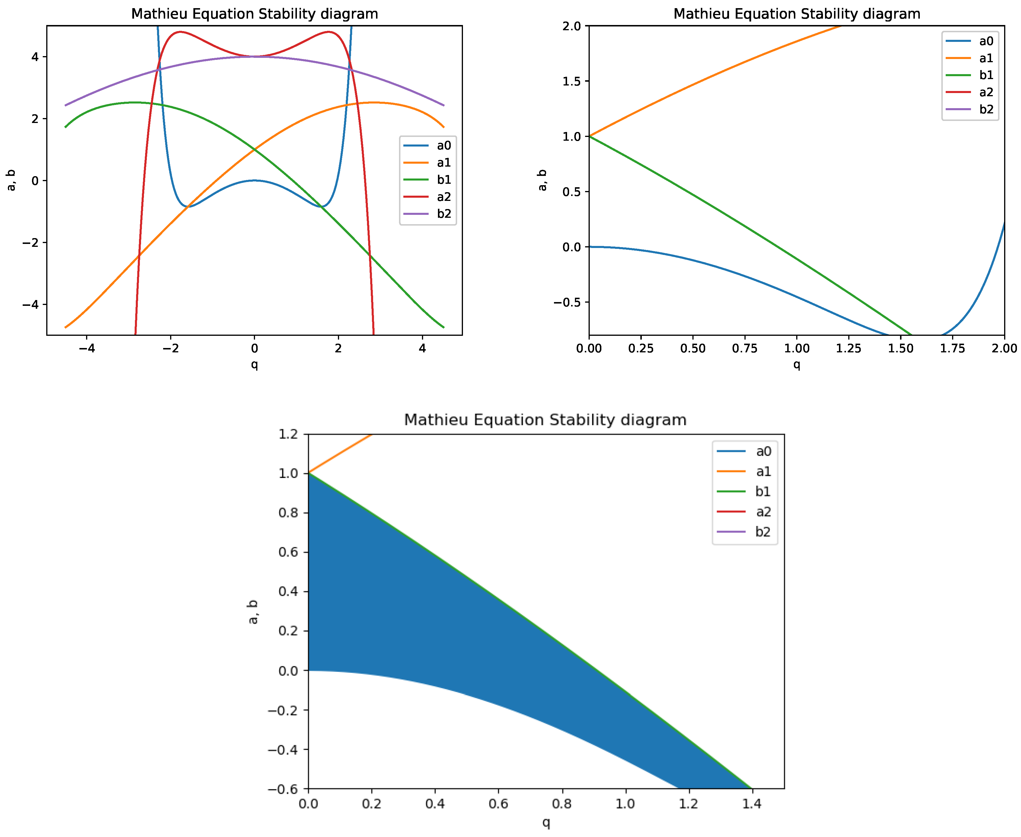
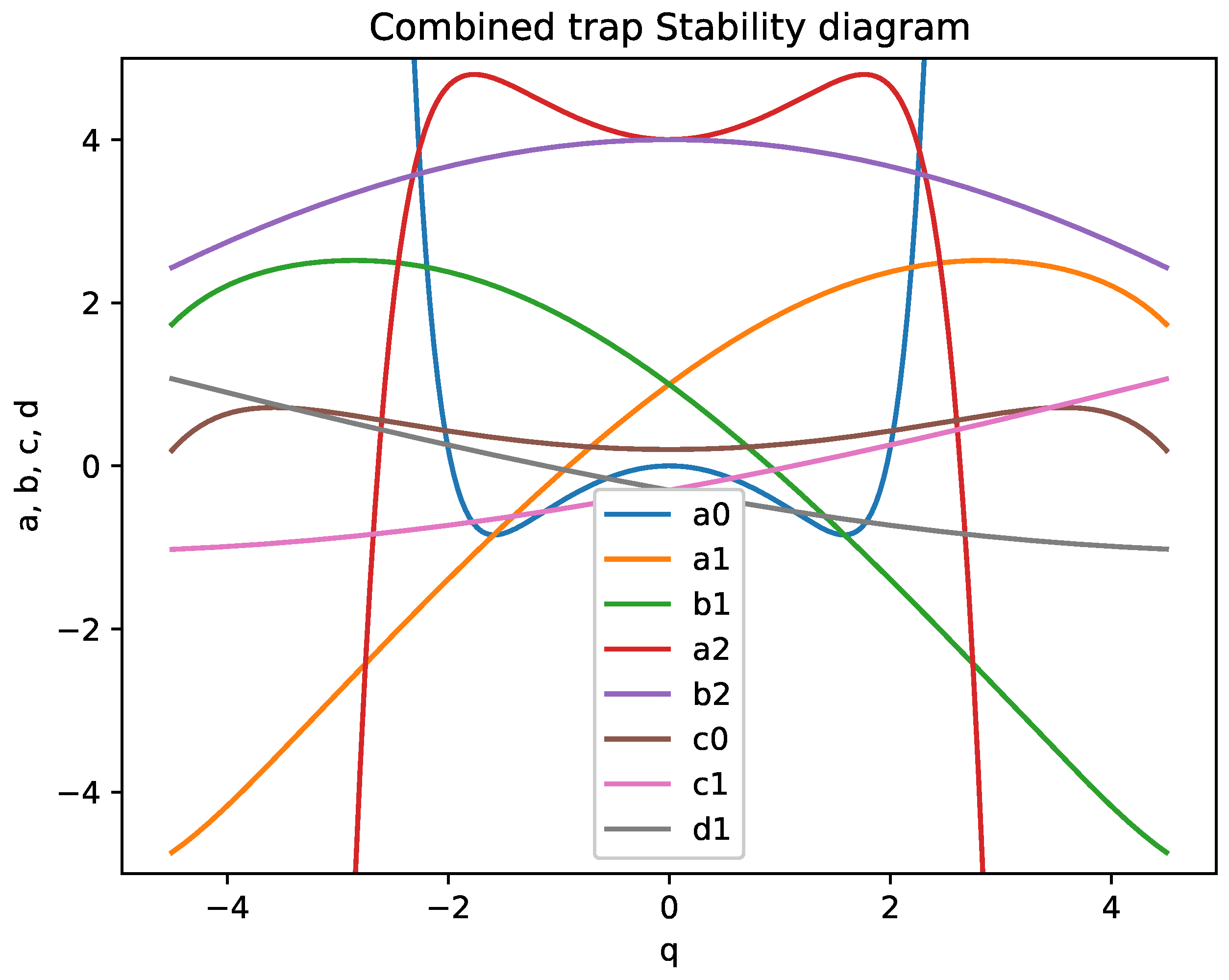
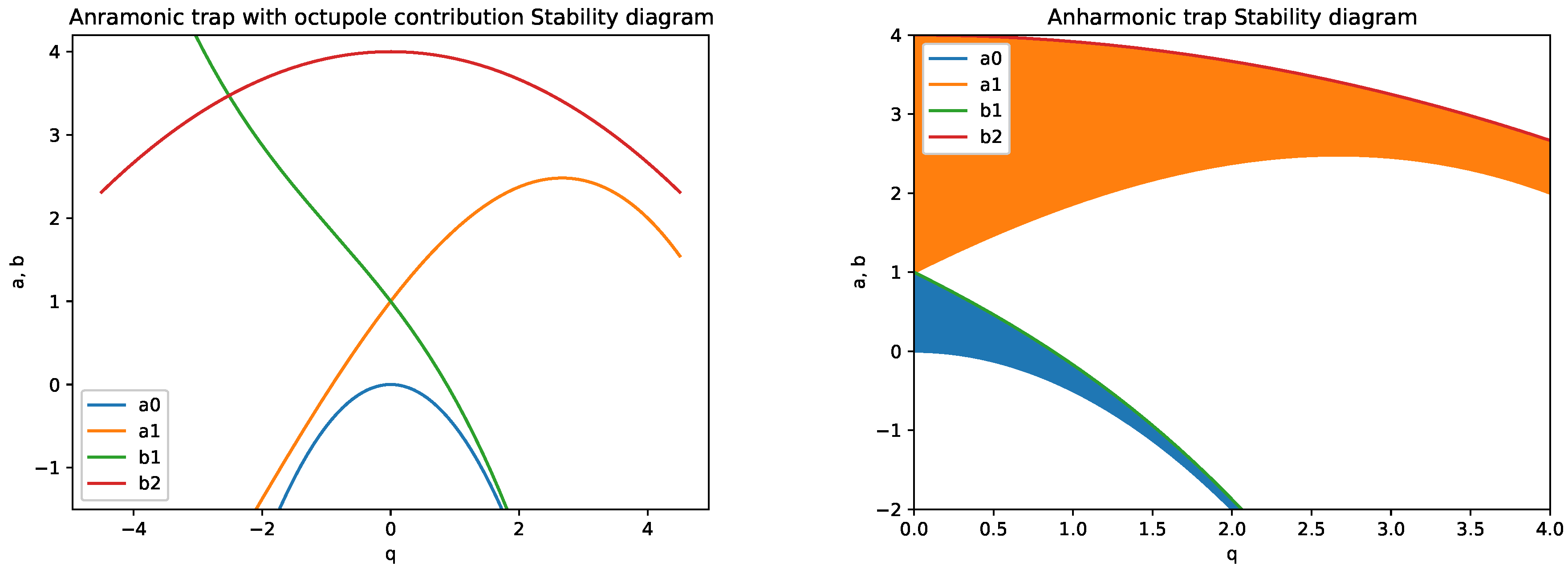
4.2. The Frontiers of the Stability Diagram for the Mathieu Equation with Nonlinear Term

This section of the paper presents the technique we have developed to derive $a_0$. The frontiers of the stability diagrams of the Mathieu equation with nonlinear terms (anharmonic perturbation) are given by Equations (64) –(67), which correspond to the following limit solutions for $q=0$:

$$a_0=0;a_1=1\mathrm{and}{z}_0=cos\tau ;a_1=-1\mathrm{and}{z}_0=sin\tau$$

(68)

The motion of a single charged particle in a nonlinear Paul trap in the presence of the damping force is theoretically investigated in [119] and the modified stability diagrams in the parameter space are calculated. The results show that the stable regions in the $a-q$ parameter plane are not only enlarged but also shifted. Our results also show that the frontiers of the stability diagrams for the Mathieu equation are shifted towards negative values of the a parameter (within the plan defined by the control parameters $a-q$). In disagreement with the pseudopotential approximation for a Paul (RF) trap [115,158], when the electric potential is described by a polynomial of rank 2 in $z^2$, by taking into account the micromotion (when not in the pseudopotential approximation), stability regions result that are qualitatively similar to those of the Mathieu equation but with frontiers that are shifted depending on the anharmonicity parameter $\lambda \left(\beta \right)$. Further on, we express Equation (63) in case $p=1$ as

$$\frac{d^2{z}_1}{d{\tau }^2}+a_0{z}_1=z_{0}cos\left(2\tau \right)-a_1{z}_0-\beta z_0^3$$

(69)

and we compute the right term for $z_0=cos\tau$. Then, the right hand side of Equation (69) is cast into

$$cos\left(2\tau \right)cos\tau -a_{1}cos\tau -\beta {cos}^3\tau$$

(70)

which can be further expressed as (see Appendix C)

$$\left(2{cos}^2\tau -1\right)cos\tau -a_{1}cos\tau -\beta {cos}^3\tau$$

(71)

One writes

$$cos3\tau =cos2\tau cos\tau -sin2\tau sin\tau =2{cos}^3\tau -cos\tau -2\left(1-{cos}^2\tau \right)cos\tau$$

(72)

as

$$cosx=\frac{e^{ix}+e^{-ix}}{2}$$

(73)

Then, one derives

$$\begin{array}{c}{\left(cosx\right)}^n=\frac{1}{2^n}\sum _{k=0}^n{C}_n^k{e}^{ix\left(n-k\right)}{e}^{-ixk}=\frac{1}{2^n}\sum _{k=0}^n{C}_n^k{e}^{ix\left(n-2k\right)}\hfill \\ \hspace{1em}\hspace{1em}\hspace{1em}\hspace{1em}\hspace{1em}\hspace{1em}\hspace{1em}\hspace{1em}\hspace{1em}\hspace{1em}\hspace{1em}\hspace{1em}\hspace{1em}\hspace{1em}=\frac{1}{2^n}\sum _{k=0}^n{C}_n^k\left[cos\left(n-2k\right)x+isin\left(n-2k\right)x\right]\hfill \end{array}$$

(74)

Hence, Equation (74) becomes

$${\left(cosx\right)}^n=\frac{1}{2^n}\sum _{k=0}^n{C}_n^{k}cos\left(n-2k\right)x$$

(75)

Using Equation (75), we infer

$$cos3\tau =4{cos}^3\tau -3cos\tau \mapsto co{s}^3\tau =\frac{1}{4}\left(cos3\tau +3cos\tau \right)$$

(76)

Then, Equation (69) becomes

$$\frac{d^2{z}_1}{d{\tau }^2}+a_0{z}_1=\left(2-\beta \right){cos}^3\tau -\left(a_1+1\right)cos\tau$$

(77)

By using Equation (76), Equation (77) changes accordingly to

$$\frac{d^2{z}_1}{d{\tau }^2}+a_0{z}_1=\left(2-\beta \right)\frac{1}{4}cos3\tau +\left(\frac{1}{2}-\frac{3}{4}\beta -a_1\right)cos\tau$$

(78)

The general solution of the harmonic oscillator (HO) writes as

$$z_{1g}=\alpha cos\tau +\beta sin\tau$$

(79)

We choose an even solution, such as $z_{1g}=\alpha cos\tau$. Then, one tries a particular solution such as

$$z_{1part}=Acos3\tau +Bcos\tau$$

(80)

with

$${\ddot{z}}_{1part}=-9Acos3\tau -Bcos\tau$$

(81)

Then, Equation (78) changes into

$$-8Acos3\tau =\frac{1}{4}\left(2-\beta \right)cos3\tau +\left(\frac{1}{2}-\frac{3}{4}\beta -a_1\right)cos\tau$$

(82)

which enables us to infer

$$a_1=\frac{1}{4}\left(2-3\beta \right),A=\frac{1}{32}\left(\beta -2\right)\Rightarrow z_1=cos\tau +\frac{1}{32}\left(\beta -2\right)cos3\tau$$

(83)

Hence, the solution of the Mathieu equation can be expressed as

$$z=z_0+z_1+\dots =1+cos\tau +\frac{1}{32}\left(\beta -2\right)cos3\tau +\dots$$

(84)

More explicit details with respect to solving the Mathieu equation by means of the perturbation theory and determining approximations to all other Mathieu functions and eigenvalues are supplied in Appendix C.

5. Discussion

An ideal IT exhibits a pure 3D quadrupole field, while the associated dynamics is characterized by the exact analytical solution of the MH equation [21,29,158]. In a quadrupole ideal IT the equations of motion are linear and uncoupled. As a matter of fact, the situation is entirely different in the case of real IT where the trapping field is far from linear due to geometric imperfections [39], such as the truncation of electrodes or geometric misalignment [165], stray electric charges, etc. These limitations superimpose weak multipole fields such as hexapole, octopole, decapole and higher-order electric fields [103,120,166,167,168]. The superposition of higher multipole fields significantly alters ion dynamics with respect to the case of a pure quadrupole trap [169,170]. The equation that characterizes ion motion in an anharmonic, real trap [56,125,163], is the nonlinear Mathieu equation which has no analytical solutions [115,129]. Furthermore, electrode misalignment results in symmetry breaking and leads to extra local minima in the trapping potential [98,165]. Trapped ion trajectories in the quadrupole, hexapole, octopole and dodecapole RF traps are investigated in [170]. A detailed analysis of the motion of trapped ions as a function of the amplitude, phase and stability of the ion’s motion is used to evaluate the experimental prospects for such traps.

This paper approaches the issues of the Hill equation solution completeness and those of periodic fundamental solutions of the Mathieu equation. We use the Floquet theorem, and based on the MH equation we find the recurrence relationship that supplies the coefficients and the characteristic exponent. We show the coefficients $c_s$ exhibit non-trivial solutions if the infinite determinant satisfies $△\left(i\mu \right)=0$ (vanishes) for noninfinite s. Then, a holomorphic function with a single pole (similar to the determinant) is introduced, and we use the Liouville theorem for complex calculus and derive the expression of the Floquet characteristic exponent. It is assumed the Floquet characteristic exponent $\mu$ is chosen to satisfy the prerequisite such that the determinant described by Equation (18) vanishes. The solution will be unbounded unless the Floquet exponent is imaginary. We supply this solution as a function of $△\left(0\right)$. To calculate this last determinant, one uses the Sträng recursion formula (method) [132], which is described in Appendix A.1.

Then, we discuss the stability of the MH equation for a trapped ion in the case of trap operating points $a,q\in \mathbb{R}$ that lie within the first stability region, pointing out when the associated dynamics are bounded or unbounded. By minimizing the parameters a and q, the coefficients $c_{2s}$ (with $s\ne 0$) of the Hill series solution rapidly converge to zero, in such a way that higher harmonics are practically insignificant and only the fundamental frequency prevails. We infer the solution of the Hill equation in such a case and find the solution by means of the pseudopotential approximation. We find both the shift in particle position and the first correction. We demonstrate that the initial conditions have no effect whatsoever on the stability of ion trajectories, but they establish their position with respect to the area located between the trap electrodes for every operating point located within a stability domain. We show the characteristic curves (which are analytical in q) are naturally introduced by means of the Sturm–Liouville (eigenvalue) problem [137,152] for the Mathieu functions $c{e}_m\left(z,q\right)$ (even) and $s{e}_m\left(z,q\right)$ (odd) [20], which are treated as characteristic functions of Equation (10) with limit conditions. These characteristic functions (curves) separate the $(a,q)$ plane into stability and instability regions, separated by the curve $\left|cosh\left(\pi \mu \right)\right|=1$ for which a stable and periodic solution of Equation (10) exists, although the general solution is unbounded. The curves characterized by integer values of $i\mu$ are called characteristic curves. We also show the periodic solutions as well as the boundaries between stability and instability regions in the $\left(a,q\right)$ parameter plane can be found by means of the Lindstedt–Poincaré method. Then, we illustrate the stability diagram for the Mathieu equation in case of an electrodynamic trap as a function of the associated eigenvalues and show the stable solution to be a superposition of harmonic motions.

In this regard, the problem of evaluating the maximum amplitude of stable oscillations under given initial conditions is approached. The maximum admits upper bounds determined by the relative position of the electrodes. To investigate ion trajectories in the phase space, we build a family of ellipses while we supply the transfer matrix and find the maximum amplitude of stable oscillations. We exemplify our analytical model for the case of a damped, kicked PO, for which we supply the general solution and discuss the frontiers of the stability domains for the homogeneous equation.

The stability diagram (associated to the Mathieu equation) that characterizes the dynamics of an ion confined within a combined quadrupole trap (a combination between a Penning and a Paul trap) is included. We illustrate the frontiers of the stability diagram for the canonical Mathieu equation for axial motion, as well as the frontiers of the stability domains for the radial trap motion, which are shown to also depend on the cyclotronic frequency.

Different ion trap geometries and electrode space arrangements are generally used (especially hyperbolic and cylindrical traps) in order to achieve a harmonic (electric) trapping potential around the trap center. Whilst hyperbolic geometries surround the trap center almost entirely, cylindrical ones usually exhibit open-endcap designs that allow better axial access to the center and enhanced interaction between levitated particles and laser beams used for cooling or manipulation [171], which makes them suited for MS, quantum optics, optical frequency metrology and quantum information processing (QIP) applications. For this reason, classical (hyperbolic) endcap electrode geometries are frequently employed when building single-ion optical clocks, as they provide certain benefits such as a saddle-shaped trapping potential which is essentially quadrupole, along with an open electrode structure that enables effective fluorescence detection [90,105]. Furthermore, a hyperbolic trap potential exhibits true azimuthal angle independence due to the electrode symmetry [172]. An open endcap trap design also exhibits a smaller quadrupole field component in the series expansion of the trap potential, while higher order terms must be considered when calculating the potential apart from the origin. Consequently, besides compensation of the effects of higher-order terms of the electric potential, some of which are approached in this paper, a careful trap design must consider and minimize issues such as potential frequency shifts and systematic errors in the atomic clock operation [72,73,173,174].

Axial stability for ion dynamics in a nonlinear Paul trap is investigated. In the case of the octopole trap (with an anharmonicity of order 4) considered, the frontiers of the stability diagram have been explicitly determined as a series expansion of the control parameters chosen. We illustrate graphically that the frontiers of the stability diagrams for the Mathieu equation with anharmonic perturbation are shifted towards negative values along the a axis, in the control parameters plan $a-q$, in agreement with [120,121]. Moreover, in the case of an octopole trap, the equations of motion are nonlinear and coupled which means that ion trajectories exhibit strong sensitivity with respect to the initial conditions. As an outcome of such a fact, it is not possible to define absolute stability conditions based only on the trap operating parameters in the stability diagram ($a,q$). The issue of dynamical stability for multiple ions, among other topics, is investigated in [31]. It is our intention to investigate the stability of ion (Coulomb) crystals used for optical clocks in the near future, taking into consideration externally forced Duffing PO as a natural model for ITs. Classical and quantum chaos is also expected to occur for specific parameters, used in numerical simulations or in the experiments performed, as well as strange attractors and fractal basin boundaries.

Both the paper submitted and the scientific literature demonstrate that geometrical imperfections play an important role in altering trap pseudo-potential, but they do not recommend corrections of the nominal trap geometry that could result in quantifiable improvements in the trapping efficiency [90]. We consider the results to be of interest for 2D and 3D ion traps used for different applications in ultrahigh-resolution spectroscopy, MS, and especially in the domain of quantum technologies (QT) based on ion traps, among which we evidence optical clocks (as extremely high-precision quantum sensors) and quantum metrology experiments.

References

1. Nayfeh, A.H.; Sanchez, N.E. Bifurcations in a forced softening duffing oscillator. Int. J. Nonlin. Mech. 1989, 24, 483–497. [Google Scholar] [CrossRef]
2. Serov, V. Fourier Series, Fourier Transform and Their Applications to Mathematical Physics; Applied Mathematical Sciences; Springer: Cham, Switzerland, 2017. [Google Scholar] [CrossRef]
3. Gadella, M.; Giacomini, H.; Lara, L. Periodic analytic approximate solutions for the Mathieu equation. Appl. Math. Comput. 2015, 271, 436–445. [Google Scholar] [CrossRef]
4. Rand, R.H. CISM Course: Time-Periodic Systems. 5–9 September 2016. Available online: http://audiophile.tam.cornell.edu/randpdf/rand_mathieu_CISM.pdf (accessed on 22 May 2024).
5. Krack, M.; Gross, J. Harmonic Balance for Nonlinear Vibration Problems; Schröder, J., Weigand, B., Eds.; Mathematical Engineering; Springer: Cham, Switzerland, 2019. [Google Scholar] [CrossRef]
6. Mathieu, E. Mémoire sur le mouvement vibratoire d’une membrane de forme elliptique. J. Math. Pures Appl. 1868, 13, 137–203. [Google Scholar]
7. Arfken, G.B.; Weber, H.J.; Harris, F.E. Mathematical Methods for Physicists, 7th ed.; Academic Press: Waltham, MA, USA, 2013; Chapter 32; pp. 1–29. Available online: https://booksite.elsevier.com/9780123846549/Chap_Mathieu.pdf (accessed on 11 May 2024).
8. Daniel, D.J. Exact solutions of Mathieu’s equation. Prog. Theor. Exp. Phys. 2020, 2020, 043A01. [Google Scholar] [CrossRef]
9. Brimacombe, C.; Corless, R.M.; Zamir, M. Computation and Applications of Mathieu Functions: A Historical Perspective. SIAM Rev. 2021, 63, 653–720. [Google Scholar] [CrossRef]
10. Wilkinson, S.A.; Vogt, N.; Golubev, D.S.; Cole, J.H. Approximate solutions to Mathieu’s equation. Phys. E Low Dimens. Syst. Nanostruct. 2018, 100, 24–30. [Google Scholar] [CrossRef]
11. Corless, R.M. An Hermite–Obreshkov method for 2nd-order linear initial-value problems for ODE. Numer. Algorithms 2024. [Google Scholar] [CrossRef]
12. Butikov, E. Analytical expressions for stability regions in the Ince–Strutt diagram of Mathieu equation. Am. J. Phys. 2018, 86, 257–267. [Google Scholar] [CrossRef]
13. Kovacic, I.; Rand, R.; Sah, S.M. Mathieu’s Equation and Its Generalizations: Overview of Stability Charts and Their Features. Appl. Mech. Rev. 2018, 70, 020802. [Google Scholar] [CrossRef]
14. Nayfeh, A.H. Introduction to Perturbation Techniques; Wiley Classics Library, Wiley: Weinheim, Germany, 2011. [Google Scholar]
15. Doroudi, A. Application of a Modified Homotopy Perturbation Method for Calculation of Secular Axial Frequencies in a Nonlinear Ion Trap with Hexapole, Octopole and Decapole Superpositions. J. Bioanal. Biomed. 2012, 4, 85–91. [Google Scholar] [CrossRef]
16. Jazar, R.N. Perturbation Methods in Science and Engineering; Springer: Cham, Switzerland, 2021. [Google Scholar] [CrossRef]
17. El-Dib, Y.O. An innovative efficient approach to solving damped Mathieu–Duffing equation with the non-perturbative technique. Commun. Nonlinear Sci. Numer. Simul. 2024, 128, 107590. [Google Scholar] [CrossRef]
18. Gadella, M.; Lara, L.P. A variational modification of the Harmonic Balance method to obtain approximate Floquet exponents. Math. Meth. Appl. Sci. 2023, 46, 8956–8974. [Google Scholar] [CrossRef]
19. McLachlan, N.W. Theory and Application of Mathieu Functions; Dover Publications: New York, NY, USA, 1964; Volume 1233. [Google Scholar]
20. Abramowitz, M.; Stegun, I.A. (Eds.) Mathieu Functions; Appl. Math. Series; US Dept. of Commerce, National Bureau of Standards: Washington, DC, USA, 1972; Volume 55, Chapter 20; pp. 722–750.
21. Major, F.G.; Gheorghe, V.N.; Werth, G. Charged Particle Traps: Physics and Techniques of Charged Particle Field Confinement; Springer Series on Atomic, Optical and Plasma Physics; Springer: Berlin/Heidelberg, Germany, 2005; Volume 37. [Google Scholar] [CrossRef]
22. Morais, J.; Porter, R.M. Reduced-quaternionic Mathieu functions, time-dependent Moisil-Teodorescu operators, and the imaginary-time wave equation. Appl. Math. Comput. 2023, 438, 127588. [Google Scholar] [CrossRef]
23. Orszag, M. Quantum Optics: Including Noise Reduction, Trapped Ions, Quantum Trajectories, and Decoherence, 3rd ed.; Springer: Cham, Switzerland, 2016. [Google Scholar] [CrossRef]
24. Birkandan, T.; Hortaçsu, M. Examples of Heun and Mathieu functions as solutions of wave equations in curved spaces. J. Phys. A Math. Theor. 2007, 40, 1105–1116. [Google Scholar] [CrossRef]
25. Quinn, T.; Perrine, R.P.; Richardson, D.C.; Barnes, R. A Symplectic Integrator for Hill’s Equations. Astron. J. 2010, 139, 803. [Google Scholar] [CrossRef]
26. Knoop, M.; Madsen, N.; Thompson, R.C. (Eds.) Physics with Trapped Charged Particles: Lectures from the Les Houches Winter School; Imperial College Press & World Scientific: London, UK, 2014. [Google Scholar] [CrossRef]
27. Knoop, M.; Madsen, N.; Thompson, R.C. (Eds.) Trapped Charged Particles: A Graduate Textbook with Problems and Solutions; Advanced Textbooks in Physics; World Scientific Europe: London, UK, 2016. [Google Scholar] [CrossRef]
28. Vasil’ev, I.A.; Kushchenko, O.M.; Rudyi, S.S.; Rozhdestvenskii, Y.V. Effective Rotational Potential of a Molecular Ions in a Plane Radio-Frequency Trap. Tech. Phys. 2019, 64, 1379–1385. [Google Scholar] [CrossRef]
29. Kajita, M. Ion Traps; IOP Publishing: Bristol, UK, 2022. [Google Scholar] [CrossRef]
30. Vogel, M. Particle Confinement in Penning Traps: An Introduction, 2nd ed.; Babb, J., Bandrauk, A.D., Bartschat, K., Joachain, C.J., Keidar, M., Lambropoulos, P., Leuchs, G., Velikovich, A., Eds.; Springer Series on Atomic, Optical, and Plasma Physics; Springer: Cham, Switzerland, 2024; Volume 100. [Google Scholar] [CrossRef]
31. Mihalcea, B.M.; Lynch, S. Investigations on Dynamical Stability in 3D Quadrupole Ion Traps. Appl. Sci. 2021, 11, 2938. [Google Scholar] [CrossRef]
32. Mihalcea, B.M.; Filinov, V.S.; Syrovatka, R.A.; Vasilyak, L.M. The physics and applications of strongly coupled Coulomb systems (plasmas) levitated in electrodynamic traps. Phys. Rep. 2023, 1016, 1–103. [Google Scholar] [CrossRef]
33. Paul, W. Electromagnetic traps for charged and neutral particles. Rev. Mod. Phys. 1990, 62, 531–540. [Google Scholar] [CrossRef]
34. Baril, M.; Septier, A. Piégeage des ions dans un champ quadrupolaire tridimensionnel à haute fréquence. Rev. Phys. Appl. 1974, 9, 525–531. [Google Scholar] [CrossRef]
35. Schulte, M.; Lörch, N.; Leroux, I.D.; Schmidt, P.O.; Hammerer, K. Quantum Algorithmic Readout in Multi-Ion Clocks. Phys. Rev. Lett. 2016, 116, 013002. [Google Scholar] [CrossRef] [PubMed]
36. Keller, J.; Burgermeister, T.; Kalincev, D.; Didier, A.; Kulosa, A.P.; Nordmann, T.; Kiethe, J.; Mehlstäubler, T.E. Controlling systematic frequency uncertainties at the 10−19 level in linear Coulomb crystals. Phys. Rev. A 2019, 99, 013405. [Google Scholar] [CrossRef]
37. Zhao, X.; Granot, O.; Douglas, D.J. Quadrupole Excitation of Ions in Linear Quadrupole Ion Traps with Added Octopole Fields. J. Am. Soc. Mass Spectrom. 2008, 19, 510–519. [Google Scholar] [CrossRef] [PubMed]
38. Austin, D.E.; Hansen, B.J.; Peng, Y.; Zhang, Z. Multipole expansion in quadrupolar devices comprised of planar electrode arrays. Int. J. Mass Spectrom. 2010, 295, 153–158. [Google Scholar] [CrossRef]
39. Wang, Y.; Zhang, X.; Feng, Y.; Shao, R.; Xiong, X.; Fang, X.; Deng, Y.; Xu, W. Characterization of geometry deviation effects on ion trap mass analysis: A comparison study. Int. J. Mass Spectrom. 2014, 370, 125–131. [Google Scholar] [CrossRef]
40. Reece, M.P.; Huntley, A.P.; Moon, A.M.; Reilly, P.T.A. Digital Mass Analysis in a Linear Ion Trap without Auxiliary Waveforms. J. Am. Soc. Mass Spectrom. 2019, 31, 103–108. [Google Scholar] [CrossRef]
41. Nolting, D.; Malek, R.; Makarov, A. Ion traps in modern mass spectrometry. Mass Spectrom. Rev. 2019, 38, 150–168. [Google Scholar] [CrossRef] [PubMed]
42. Mandal, P.; Mukherjee, M. Non-degenerate dodecapole resonances in an asymmetric linear ion trap of round rod geometry. Int. J. Mass Spectrom. 2024, 498, 117217. [Google Scholar] [CrossRef]
43. Kaur Kohli, R.; Van Berkel, G.J.; Davies, J.F. An Open Port Sampling Interface for the Chemical Characterization of Levitated Microparticles. Anal. Chem. 2022, 94, 3441–3445. [Google Scholar] [CrossRef]
44. Harris, W.A.; Reilly, P.T.A.; Whitten, W.B. Detection of Chemical Warfare-Related Species on Complex Aerosol Particles Deposited on Surfaces Using an Ion Trap-Based Aerosol Mass Spectrometer. Anal. Chem. 2007, 79, 2354–2358. [Google Scholar] [CrossRef]
45. Pan, Y.L.; Wang, C.; Hill, S.C.; Coleman, M.; Beresnev, L.A.; Santarpia, J.L. Trapping of individual airborne absorbing particles using a counterflow nozzle and photophoretic trap for continuous sampling and analysis. Appl. Phys. Lett. 2014, 104, 113507. [Google Scholar] [CrossRef]
46. Fachinger, J.R.W.; Gallavardin, S.J.; Helleis, F.; Fachinger, F.; Drewnick, F.; Borrmann, S. The ion trap aerosol mass spectrometer: Field intercomparison with the ToF-AMS and the capability of differentiating organic compound classes via MS-MS. Atmos. Meas. Tech. 2017, 10, 1623–1637. [Google Scholar] [CrossRef]
47. Rajagopal, V.; Stokes, C.; Ferzoco, A. A Linear Ion Trap with an Expanded Inscribed Diameter to Improve Optical Access for Fluorescence Spectroscopy. J. Am. Soc. Mass Spectrom. 2018, 29, 260–269. [Google Scholar] [CrossRef] [PubMed]
48. Johnston, M.V.; Kerecman, D.E. Molecular Characterization of Atmospheric Organic Aerosol by Mass Spectrometry. Annu. Rev. Anal. Chem. 2019, 12, 247–274. [Google Scholar] [CrossRef] [PubMed]
49. Snyder, D.T.; Szalwinski, L.J.; St. John, Z.; Cooks, R.G. Two-Dimensional Tandem Mass Spectrometry in a Single Scan on a Linear Quadrupole Ion Trap. Anal. Chem. 2019, 91, 13752–13762. [Google Scholar] [CrossRef] [PubMed]
50. Newsome, G.A.; Rosen, E.P.; Kamens, R.M.; Glish, G.L. Real-time Detection and Tandem Mass Spectrometry of Secondary Organic Aerosols with a Quadrupole Ion Trap. ChemRxiv 2020. [Google Scholar] [CrossRef]
51. Cho, H.; Kim, J.; Kwak, N.; Kwak, H.; Son, T.; Lee, D.; Park, K. Application of Single-Particle Mass Spectrometer to Obtain Chemical Signatures of Various Combustion Aerosols. Int. J. Environ. Res. Pub. Health 2021, 18, 11580. [Google Scholar] [CrossRef]
52. Gonzalez, L.E.; Szalwinski, L.J.; Marsh, B.M.; Wells, J.M.; Cooks, R.G. Immediate and sensitive detection of sporulated Bacillus subtilis by microwave release and tandem mass spectrometry of dipicolinic acid. Analyst 2021, 146, 7104–7108. [Google Scholar] [CrossRef]
53. Wineland, D.J.; Monroe, C.; Meekhof, D.M.; King, B.E.; Leibfried, D.; Itano, W.M.; Bergquist, J.C.; Berkeland, D.; Bollinger, J.J.; Miller, J. Quantum state manipulation of trapped atomic ions. Proc. R. Soc. Lond. A 1998, 454, 411–429. [Google Scholar] [CrossRef]
54. Blaum, K.; Novikov, Y.N.; Werth, G. Penning traps as a versatile tool for precise experiments in fundamental physics. Contemp. Phys. 2010, 51, 149–175. [Google Scholar] [CrossRef]
55. Wineland, D.J. Nobel Lecture: Superposition, entanglement, and raising Schrödinger’s cat. Rev. Mod. Phys. 2013, 85, 1103–1114. [Google Scholar] [CrossRef]
56. Mihalcea, B.M. Squeezed coherent states of motion for ions confined in quadrupole and octupole ion traps. Ann. Phys. 2018, 388, 100–113. [Google Scholar] [CrossRef]
57. Wan, Y.; Jördens, R.; Erickson, S.D.; Wu, J.J.; Bowler, R.; Tan, T.R.; Hou, P.Y.; Wineland, D.J.; Wilson, A.C.; Leibfried, D. Ion Transport and Reordering in a 2D Trap Array. Adv. Quantum Technol. 2020, 3, 2000028. [Google Scholar] [CrossRef]
58. Mihalcea, B.M. Quasienergy operators and generalized squeezed states for systems of trapped ions. Ann. Phys. 2022, 442, 169826. [Google Scholar] [CrossRef]
59. Häffner, H.; Roos, C.F.; Blatt, R. Quantum computing with trapped ions. Phys. Rep. 2008, 469, 155–203. [Google Scholar] [CrossRef]
60. Pagano, G.; Hess, P.W.; Kaplan, H.B.; Tan, W.L.; Richerme, P.; Becker, P.; Kyprianidis, A.; Zhang, J.; Birckelbaw, E.; Hernandez, M.R.; et al. Cryogenic trapped-ion system for large scale quantum simulation. Quantum Sci. Technol. 2018, 4, 014004. [Google Scholar] [CrossRef]
61. Bruzewicz, C.D.; Chiaverini, J.; McConnell, R.; Sage, J.M. Trapped-ion quantum computing: Progress and challenges. Appl. Phys. Rev. 2019, 6, 021314. [Google Scholar] [CrossRef]
62. Mokhberi, A.; Hennrich, M.; Schmidt-Kaler, F. Chapter Four-Trapped Rydberg ions: A new platform for quantum information processing. In Advances in Atomic, Molecular, and Optical Physics; Dimauro, L.F., Perrin, H., Yelin, S.F., Eds.; Academic Press: Cambridge, MA, USA; Volume 69, pp. 233–306. [CrossRef]
63. LaPierre, R. Introduction to Quantum Computing; The Materials Research Society Series; Springer: Cham, Switzerland, 2021. [Google Scholar] [CrossRef]
64. Reiter, F.; Sørensen, A.S.; Zoller, P.; Muschik, C.A. Dissipative quantum error correction and application to quantum sensing with trapped ions. Nat. Commun. 2017, 8, 1822. [Google Scholar] [CrossRef] [PubMed]
65. Fountas, P.N.; Poggio, M.; Willitsch, S. Classical and quantum dynamics of a trapped ion coupled to a charged nanowire. New J. Phys. 2019, 21, 013030. [Google Scholar] [CrossRef]
66. Wolf, F.; Schmidt, P.O. Quantum sensing of oscillating electric fields with trapped ions. Meas. Sens. 2021, 18, 100271. [Google Scholar] [CrossRef]
67. Affolter, M.; Ge, W.; Bullock, B.; Burd, S.C.; Gilmore, K.A.; Lilieholm, J.F.; Carter, A.L.; Bollinger, J.J. Toward improved quantum simulations and sensing with trapped two-dimensional ion crystals via parametric amplification. Phys. Rev. A 2023, 107, 032425. [Google Scholar] [CrossRef]
68. Sinclair, A. An Introduction to Trapped Ions, Scalability and Quantum Metrology. In Quantum Information and Coherence; Andersson, E., Öhberg, P., Eds.; Scottish Graduate Series; Springer: Berlin/Heidelberg, Germany, 2011; Volume 67, pp. 211–246. [Google Scholar] [CrossRef]
69. Colombo, S.; Pedrozo-Peñafiel, E.; Adiyatullin, A.F.; Li, Z.; Mendez, E.; Shu, C.; Vuletić, V. Time-reversal-based quantum metrology with many-body entangled states. Nat. Phys. 2022, 18, 925–930. [Google Scholar] [CrossRef]
70. Lee, D.; Watkins, J.; Frame, D.; Given, G.; He, R.; Li, N.; Lu, B.N.; Sarkar, A. Time fractals and discrete scale invariance with trapped ions. Phys. Rev. A 2019, 100, 011403. [Google Scholar] [CrossRef]
71. Li, T.; Gong, Z.X.; Yin, Z.Q.; Quan, H.T.; Yin, X.; Zhang, P.; Duan, L.M.; Zhang, X. Space-Time Crystals of Trapped Ions. Phys. Rev. Lett. 2012, 109, 163001. [Google Scholar] [CrossRef] [PubMed]
72. Vanier, J.; Tomescu, C. The Quantum Physics of Atomic Frequency Standards: Recent Developments; CRC Press: Boca Raton, FL, USA, 2015. [Google Scholar] [CrossRef]
73. Ludlow, A.D.; Boyd, M.M.; Ye, J.; Peik, E.; Schmidt, P.O. Optical atomic clocks. Rev. Mod. Phys. 2015, 87, 637–701. [Google Scholar] [CrossRef]
74. Nordmann, T.; Didier, A.; Doležal, M.; Balling, P.; Burgermeister, T.; Mehlstäubler, T.E. Sub-kelvin temperature management in ion traps for optical clocks. Rev. Sci. Instrum. 2020, 91, 111301. [Google Scholar] [CrossRef] [PubMed]
75. Hausser, H.N.; Keller, J.; Nordmann, T.; Bhatt, N.M.; Kiethe, J.; Liu, H.; von Boehn, M.; Rahm, J.; Weyers, S.; Benkler, E.; et al. An 115In+172Yb+ Coulomb crystal clock with 2.5 ×10 −18 systematic uncertainty. arXiv 2024, arXiv:2402.16807. [Google Scholar] [CrossRef]
76. Barontini, G.; Blackburn, L.; Boyer, V.; Butuc-Mayer, F.; Calmet, X.; López-Urrutia, J.R.C.; Curtis, E.A.; Darquié, B.; Dunningham, J.; Fitch, N.J.; et al. Measuring the stability of fundamental constants with a network of clocks. EPJ Quant. Technol. 2022, 9, 12. [Google Scholar] [CrossRef]
77. Tsai, Y.D.; Eby, J.; Safronova, M.S. Direct detection of ultralight dark matter bound to the Sun with space quantum sensors. Nat. Astron. 2023, 7, 113–121. [Google Scholar] [CrossRef]
78. Safronova, M.S.; Budker, D.; DeMille, D.; Kimball, D.F.J.; Derevianko, A.; Clark, C.W. Search for new physics with atoms and molecules. Rev. Mod. Phys. 2018, 90, 025008. [Google Scholar] [CrossRef]
79. Schkolnik, V.; Budker, D.; Fartmann, O.; Flambaum, V.; Hollberg, L.; Kalaydzhyan, T.; Kolkowitz, S.; Krutzik, M.; Ludlow, A.; Newbury, N.; et al. Optical atomic clock aboard an Earth-orbiting space station (OACESS): Enhancing searches for physics beyond the standard model in space. Quantum Sci. Technol. 2022, 8, 014003. [Google Scholar] [CrossRef]
80. Derevianko, A.; Gibble, K.; Hollberg, L.; Newbury, N.R.; Oates, C.; Safronova, M.S.; Sinclair, L.C.; Yu, N. Fundamental physics with a state-of-the-art optical clock in space. Quantum Sci. Technol. 2022, 7, 044002. [Google Scholar] [CrossRef]
81. McGrew, W.F.; Zhang, X.; Leopardi, H.; Fasano, R.J.; Nicolodi, D.; Beloy, K.; Yao, J.; Sherman, J.A.; Schäffer, S.A.; Savory, J.; et al. Towards the optical second: Verifying optical clocks at the SI limit. Optica 2019, 6, 448–454. [Google Scholar] [CrossRef]
82. Shen, Q.; Guan, J.Y.; Ren, J.G.; Zeng, T.; Hou, L.; Li, M.; Cao, Y.; Han, J.J.; Lian, M.Z.; Chen, Y.W.; et al. Free-space dissemination of time and frequency with 10−19 instability over 113 km. Nature 2022, 610, 661–666. [Google Scholar] [CrossRef] [PubMed]
83. Kim, M.E.; McGrew, W.F.; Nardelli, N.V.; Clements, E.R.; Hassan, Y.S.; Zhang, X.; Valencia, J.L.; Leopardi, H.; Hume, D.B.; Fortier, T.M.; et al. Improved interspecies optical clock comparisons through differential spectroscopy. Nat. Phys. 2023, 19, 25–29. [Google Scholar] [CrossRef]
84. Peik, E. Optical Atomic Clocks. In Photonic Quantum Technologies; Benyoucef, M., Ed.; Wiley: Weinheim, Germany, 2023; Chapter 14; pp. 333–348. [Google Scholar] [CrossRef]
85. Dimarcq, N.; Gertsvolf, M.; Mileti, G.; Bize, S.; Oates, C.W.; Peik, E.; Calonico, D.; Ido, T.; Tavella, P.; Meynadier, F.; et al. Roadmap towards the redefinition of the second. Metrologia 2024, 61, 012001. [Google Scholar] [CrossRef]
86. Tomescu, C.; Giurgiu, L. Atomic Clocks and Time Keeping in Romania. Rom. Rep. Phys. 2018, 70, 205. Available online: https://rrp.nipne.ro/2018/AN70205.pdf (accessed on 11 May 2024).
87. Itano, W.M.; Bergquist, J.C.; Bollinger, J.J.; Gilligan, J.M.; Heinzen, D.J.; Moore, F.L.; Raizen, M.G.; Wineland, D.J. Quantum projection noise: Population fluctuations in two-level systems. Phys. Rev. A 1993, 47, 3554–3570. [Google Scholar] [CrossRef]
88. Wineland, D.J.; Bollinger, J.J.; Itano, W.M.; Heinzen, D.J. Squeezed atomic states and projection noise in spectroscopy. Phys. Rev. A 1994, 50, 67–88. [Google Scholar] [CrossRef]
89. Wolf, F.; Shi, C.; Heip, J.C.; Gessner, M.; Pezzè, L.; Smerzi, A.; Schulte, M.; Hammerer, K.; Schmidt, P.O. Motional Fock states for quantum-enhanced amplitude and phase measurements with trapped ions. Nat. Commun. 2019, 10, 2929. [Google Scholar] [CrossRef]
90. Spampinato, A.; Stacey, J.; Mulholland, S.; Robertson, B.I.; Klein, H.A.; Huang, G.; Barwood, G.P.; Gill, P. An ion trap design for a space-deployable strontium-ion optical clock. Proc. R. Soc. A 2024, 480, 20230593. [Google Scholar] [CrossRef]
91. Zhiqiang, Z.; Arnold, K.J.; Kaewuam, R.; Barrett, M.D. 176Lu+ clock comparison at the 10−18 level via correlation spectroscopy. Sci. Adv. 2023, 9, eadg1971. [Google Scholar] [CrossRef] [PubMed]
92. Caldwell, E.D.; Sinclair, L.C.; Deschenes, J.D.; Giorgetta, F.; Newbury, N.R. Application of quantum-limited optical time transfer to space-based optical clock comparisons and coherent networks. APL Photonics 2024, 9, 016112. [Google Scholar] [CrossRef]
93. Joshi, M.K.; Satyajit, K.T.; Rao, P.M. Influence of a geometrical perturbation on the ion dynamics in a 3D Paul trap. Nucl. Instrum. Methods Phys. Res. A 2015, 800, 111–118. [Google Scholar] [CrossRef]
94. Tian, Y.; Decker, T.K.; McClellan, J.S.; Wu, Q.; De la Cruz, A.; Hawkins, A.R.; Austin, D.E. Experimental Observation of the Effects of Translational and Rotational Electrode Misalignment on a Planar Linear Ion Trap Mass Spectrometer. J. Am. Soc. Mass. Spectrom. 2018, 29, 1376–1385. [Google Scholar] [CrossRef] [PubMed]
95. Alheit, R.; Kleineidam, S.; Vedel, F.; Vedel, M.; Werth, G. Higher order non-linear resonances in a Paul trap. Int. J. Mass Spectrom. Ion Proc. 1996, 154, 155–169. [Google Scholar] [CrossRef]
96. Takai, R.; Nakayama, K.; Saiki, W.; Ito, K.; Okamoto, H. Nonlinear Resonance Effects in a Linear Paul Trap. J. Phys. Soc. Japan 2007, 76, 014802. [Google Scholar] [CrossRef]
97. Xiong, C.; Zhou, X.; Zhang, N.; Zhan, L.; Chen, Y.; Nie, Z. Nonlinear Ion Harmonics in the Paul Trap with Added Octopole Field: Theoretical Characterization and New Insight into Nonlinear Resonance Effect. J. Am. Soc. Mass Spectrom. 2016, 27, 344–351. [Google Scholar] [CrossRef]
98. Marchenay, M.; Pedregosa-Gutierrez, J.; Knoop, M.; Houssin, M.; Champenois, C. An analytical approach to symmetry breaking in multipole RF-traps. Quantum Sci. Technol. 2021, 6, 024016. [Google Scholar] [CrossRef]
99. Shaikh, F.A.; Ozakin, A. Stability analysis of ion motion in asymmetric planar ion traps. J. Appl. Phys. 2012, 112, 074904. [Google Scholar] [CrossRef]
100. Wu, H.Y.; Xie, Y.; Wan, W.; Chen, L.; Zhou, F.; Feng, M. A complicated Duffing oscillator in the surface-electrode ion trap. Appl. Phys. B 2014, 114, 81–88. [Google Scholar] [CrossRef]
101. Ghosh, I.; Saxena, V.; Krishnamachari, A. Resonance Curves and Jump Frequencies in a Dual-Frequency Paul Trap on Account of Octopole Field Imperfection. IEEE Trans. Plasma Sci. 2023, 51, 1924–1931. [Google Scholar] [CrossRef]
102. Mihalcea, B.M.; Visan, G.T.; Giurgiu, L.C.; Radan, S. Optimization of ion trap geometries and of the signal to noise ratio for high resolution spectroscopy. J. Optoelectron. Adv. Mat. 2008, 10, 1994–1998. Available online: https://old.joam.inoe.ro/download.php?idu=1538 (accessed on 11 May 2024).
103. Pedregosa, J.; Champenois, C.; Houssin, M.; Knoop, M. Anharmonic contributions in real RF linear quadrupole traps. Int. J. Mass Spectrom. 2010, 290, 100–105. [Google Scholar] [CrossRef]
104. Home, J.P.; Hanneke, D.; Jost, J.D.; Leibfried, D.; Wineland, D.J. Normal modes of trapped ions in the presence of anharmonic trap potentials. New J. Phys. 2011, 13, 073026. [Google Scholar] [CrossRef]
105. Lindvall, T.; Hanhijärvi, K.J.; Fordell, T.; Wallin, A.E. High-accuracy determination of Paul-trap stability parameters for electric-quadrupole-shift prediction. J. Appl. Phys. 2022, 132, 124401. [Google Scholar] [CrossRef]
106. Huang, Y.; Zhang, B.; Zeng, M.; Hao, Y.; Ma, Z.; Zhang, H.; Guan, H.; Chen, Z.; Wang, M.; Gao, K. Liquid-Nitrogen-Cooled Ca+ Optical Clock with Systematic Uncertainty of 3 × 10⁻¹⁸. Phys. Rev. Appl. 2022, 17, 034041. [Google Scholar] [CrossRef]
107. Leibrandt, D.R.; Porsev, S.G.; Cheung, C.; Safronova, M.S. Prospects of a thousand-ion Sn2+ Coulomb-crystal clock with sub-10−19 inaccuracy. arXiv 2022, arXiv:2205.15484. [Google Scholar] [CrossRef]
108. Martínez-Lahuerta, V.J.; Eilers, S.; Mehlstäubler, T.E.; Schmidt, P.O.; Hammerer, K. Ab initio quantum theory of mass defect and time dilation in trapped-ion optical clocks. Phys. Rev. A 2022, 106, 032803. [Google Scholar] [CrossRef]
109. Mehta, K.K.; Zhang, C.; Malinowski, M.; Nguyen, T.L.; Stadler, M.; Home, J.P. Integrated optical multi-ion quantum logic. Nature 2020, 586, 533–537. [Google Scholar] [CrossRef]
110. Sutherland, R.T.; Yu, Q.; Beck, K.M.; Häffner, H. One- and two-qubit gate infidelities due to motional errors in trapped ions and electrons. Phys. Rev. A 2022, 105, 022437. [Google Scholar] [CrossRef]
111. Fan, M.; Holliman, C.A.; Shi, X.; Zhang, H.; Straus, M.W.; Li, X.; Buechele, S.W.; Jayich, A.M. Optical Mass Spectrometry of Cold RaOH+ and RaOCH3+. Phys. Rev. Lett. 2021, 126, 023002. [Google Scholar] [CrossRef] [PubMed]
112. Landau, A.; Eduardus.; Behar, D.; Wallach, E.R.; Pašteka, L.F.; Faraji, S.; Borschevsky, A.; Shagam, Y. Chiral molecule candidates for trapped ion spectroscopy by ab initio calculations: From state preparation to parity violation. J. Chem. Phys. 2023, 159, 114307. [Google Scholar] [CrossRef] [PubMed]
113. Rajanbabu, N.; Marathe, A.; Chatterjee, A.; Menon, A.G. Multiple scales analysis of early and delayed boundary ejection in Paul traps. Int. J. Mass Spectrom. 2007, 261, 170–182. [Google Scholar] [CrossRef]
114. Wang, Y.; Huang, Z.; Jiang, Y.; Xiong, X.; Deng, Y.; Fang, X.; Xu, W. The coupling effects of hexapole and octopole fields in quadrupole ion traps: A theoretical study. J. Mass Spectrom. 2013, 48, 937–944. [Google Scholar] [CrossRef] [PubMed]
115. Xiong, C.; Zhou, X.; Zhang, N.; Zhan, L.; Chen, Y.; Chen, S.; Nie, Z. A Theoretical Method for Characterizing Nonlinear Effects in Paul Traps with Added Octopole Field. J. Am. Soc. Mass Spectrom. 2015, 26, 1338–1348. [Google Scholar] [CrossRef] [PubMed]
116. Moatimid, G.M.; Amer, T.S.; Amer, W.S. Dynamical analysis of a damped harmonic forced duffing oscillator with time delay. Sci. Rep. 2023, 13, 6507. [Google Scholar] [CrossRef] [PubMed]
117. Kovacic, I.; Brenner, M.J. (Eds.) The Duffing Equation: Nonlinear Oscillations and their Behaviour; Theoretical, Computational, and Statistical Physics; Wiley: Chichester, UK, 2011. [Google Scholar] [CrossRef]
118. Strogatz, S.H. Nonlinear Dynamics and Chaos: With Applications to Physics, Biology, Chemistry, and Engineering, 2nd ed.; Studies in Nonlinearity; CRC Press: Boca Raton, FL, USA, 2015. [Google Scholar] [CrossRef]
119. Hasegawa, T.; Uehara, K. Dynamics of a single particle in a Paul trap in the presence of the damping force. Appl. Phys. B 1995, 61, 159–163. [Google Scholar] [CrossRef]
120. Sevugarajan, S.; Menon, A.G. Frequency perturbation in nonlinear Paul traps: A simulation study of the effect of geometric aberration, space charge, dipolar excitation, and damping on ion axial secular frequency. Int. J. Mass Spectrom. 2000, 197, 263–278. [Google Scholar] [CrossRef]
121. Sevugarajan, S.; Menon, A.G. Transition curves and iso-βu lines in nonlinear Paul traps. Int. J. Mass Spectrom. 2002, 218, 181–196. [Google Scholar] [CrossRef]
122. Zhou, X.; Zhu, Z.; Xiong, C.; Chen, R.; Xu, W.; Qiao, H.; Peng, W.P.; Nie, Z.; Chen, Y. Characteristics of stability boundary and frequency in nonlinear ion trap mass spectrometer. J. Am. Soc. Mass Spectrom. 2010, 21, 1588–1595. [Google Scholar] [CrossRef] [PubMed]
123. Ishizaki, R.; Sata, H.; Shoji, T. Chaos-Induced Diffusion in a Nonlinear Dissipative Mathieu Equation for a Charged Fine Particle in an AC Trap. J. Phys. Soc. Jpn. 2011, 80, 044001. [Google Scholar] [CrossRef]
124. Brouwers, J.J.H. Asymptotic solutions for Mathieu instability under random parametric excitation and nonlinear damping. Phys. D 2011, 240, 990–1000. [Google Scholar] [CrossRef]
125. Mihalcea, B.M.; Vişan, G.G. Nonlinear ion trap stability analysis. Phys. Scr. 2010, T140, 014057. [Google Scholar] [CrossRef]
126. Rybin, V.; Rudyi, S.; Rozhdestvensky, Y. Nano- and microparticle nonlinear damping identification in quadrupole trap. Int. J. Non-Linear Mech. 2022, 147, 104227. [Google Scholar] [CrossRef]
127. Nayfeh, A.H.; Balachandran, B. Applied Nonlinear Dynamics: Analytical, Computational, and Experimental Methods, 2nd ed.; Wiley Series in Nonlinear Science; Wiley-VCH: Weinheim, Germany, 2004. [Google Scholar] [CrossRef]
128. Kyzioł, J.; Okniński, A. Duffing-type equations: Singular points of amplitude profiles and bifurcations. Acta Phys. Pol. B 2021, 52, 1239–1262. [Google Scholar] [CrossRef]
129. El Fakkousy, I.; Zouhairi, B.; Benmalek, M.; Kharbach, J.; Rezzouk, A.; Ouazzani-Jamil, M. Classical and quantum integrability of the three-dimensional generalized trapped ion Hamiltonian. Chaos Solit. Fractals 2022, 161, 112361. [Google Scholar] [CrossRef]
130. Mihalcea, B.M. Study of quasiclassical dynamics of trapped ions using the coherent state formalism and associated algebraic groups. Rom. J. Phys. 2017, 62, 113. Available online: https://www.nipne.ro/rjp/2017_62_5-6/RomJPhys.62.113.pdf (accessed on 11 May 2024).
131. Rudyi, S.; Vasilyev, M.; Rybin, V.; Rozhdestvensky, Y. Stability problem in 3D multipole ion traps. Int. J. Mass Spectrom. 2022, 479, 116894. [Google Scholar] [CrossRef]
132. Sträng, J.E. On the characteristic exponents of Floquet solutions to the Mathieu equation. Bull. Acad. R. Belg. 2005, 16, 269–287. [Google Scholar] [CrossRef]
133. Rudyi, S.S.; Rybin, V.V.; Semynin, M.S.; Shcherbinin, D.P.; Rozhdestvensky, Y.V.; Ivanov, A.V. Period-doubling bifurcation in surface radio-frequency trap: Transition to chaos through Feigenbaum scenario. Chaos 2023, 33, 093133. [Google Scholar] [CrossRef] [PubMed]
134. Hill, G.W. On the part of the motion of lunar perigee which is a function of the mean motions of the sun and moon. Acta Math. 1886, 8, 1–36. [Google Scholar] [CrossRef]
135. Viswanath, D. The Lindstedt–Poincaré Technique as an Algorithm for Computing Periodic Orbits. SIAM Rev. 2001, 43, 478–495. [Google Scholar] [CrossRef]
136. Magnus, W.; Winkler, S. Hill’s Equation; Interscience Tracts in Pure and Applied Mathematics; Wiley: New York, NY, USA, 1966; Volume 20. [Google Scholar] [CrossRef]
137. Whittaker, E.T.; Watson, G.N. A Course of Modern Analysis, 5th ed.; Moll, V.H., Ed.; Cambridge University Press: Cambridge, UK, 2021. [Google Scholar] [CrossRef]
138. Wilson, E.; Holzer, B.J. Beam Dynamics. In Particle Physics Reference Library: Volume 3: Accelerators and Colliders; Myers, S., Schopper, H., Eds.; Springer International Publishing: Cham, Switzerland, 2020; pp. 15–50. [Google Scholar] [CrossRef]
139. Rodriguez, A.; Collado, J. Periodic Solutions in Non-Homogeneous Hill Equation. Nonlinear Dyn. Syst. Theory 2020, 20, 78–91. Available online: https://www.e-ndst.kiev.ua/v20n1/7(71).pdf (accessed on 11 May 2024).
140. Brillouin, L. A practical method for solving Hill’s equation. Quart. Appl. Math. 1948, 6, 167–178. [Google Scholar] [CrossRef]
141. Moussa, R.A. Generalization of Ince’s Equation. J. Appl. Math. Phys. 2014, 2, 1171–1182. [Google Scholar] [CrossRef]
142. Wolf, G. Mathieu Functions and Hill’s Equation. In NIST Handbook of Mathematical Functions; Olver, F.W.J., Lozier, D.W., Boisvert, R.F., Clark, C.W., Eds.; NIST & Cambridge University Press: New York, NY, USA, 2010; Chapter 28; pp. 651–681. [Google Scholar]
143. Landa, H.; Drewsen, M.; Reznik, B.; Retzker, A. Modes of oscillation in radiofrequency Paul traps. New J. Phys. 2012, 14, 093023. [Google Scholar] [CrossRef]
144. Ck Function. Available online: https://mathworld.wolfram.com/C-kFunction.html (accessed on 2 May 2024).
145. Landa, H.; Drewsen, M.; Reznik, B.; Retzker, A. Classical and quantum modes of coupled Mathieu equations. J. Phys. A Math. Theor. 2012, 45, 455305. [Google Scholar] [CrossRef]
146. Frenkel, D.; Portugal, R. Algebraic methods to compute Mathieu functions. J. Phys. A Math. Gen. 2001, 34, 3541–3551. [Google Scholar] [CrossRef]
147. Wong, C.W. Introduction to Mathematical Physics: Methods and Concepts, 2nd ed.; Oxford University Press: Oxford, UK, 2013. [Google Scholar] [CrossRef]
148. Gezerlis, A. Numerical Methods in Physics with Python, 2nd ed.; Cambridge University Press: Cambridge, UK, 2023. [Google Scholar] [CrossRef]
149. Jones, T. Mathieu’s Equations and the Ideal RF-Paul Trap. Available online: http://einstein.drexel.edu/~tim/open/mat/mat.pdf (accessed on 21 May 2024).
150. Weyl, H. Meromorphic Functions and Analytic Curves; Annals of Mathematics Studies, Princeton University Press—De Gruyter: Princeton, NJ, USA, 2016; Volume 12. [Google Scholar] [CrossRef]
151. Meromorphic Function. Available online: https://mathworld.wolfram.com/MeromorphicFunction.html (accessed on 2 May 2024).
152. Canosa, J. Numerical solution of Mathieu’s equation. J. Computat. Phys. 1971, 7, 255–272. [Google Scholar] [CrossRef]
153. Bibby, M.M.; Peterson, A.F. Accurate Computation of Mathieu Functions; Balanis, C.A., Ed.; Synthesis Lectures on Computational Electromagnetics; Morgan & Claypool: San Rafael, CA, USA, 2014; Volume Lecture 32. [Google Scholar] [CrossRef]
154. Gheorghe, V.N.; Giurgiu, L.; Stoican, O.; Cacicovschi, D.; Molnar, R.; Mihalcea, B. Ordered Structures in a Variable Length AC Trap. Acta Phys. Pol. A 1998, 93, 625–629. [Google Scholar] [CrossRef]
155. Kotana, A.N.; Mohanty, A.K. Computation of Mathieu stability plot for an arbitrary toroidal ion trap mass analyser. Int. J. Mass Spectrom. 2017, 414, 13–22. [Google Scholar] [CrossRef]
156. Wuerker, R.F.; Shelton, H.; Langmuir, R.V. Electrodynamic Containment of Charged Particles. J. Appl. Phys. 1959, 30, 342–349. [Google Scholar] [CrossRef]
157. Dehmelt, H. Radiofrequency Spectroscopy of Stored Ions I: Storage. In Advances in Atomic and Molecular Physics; Academic Press: Cambridge, MA, USA, 1968; Volume 3, pp. 53–72. [Google Scholar] [CrossRef]
158. March, R.E.; Todd, J.F.J. Quadrupole Ion Trap Mass Spectrometry, 2nd ed.; Winefordner, J.D., Ed.; Chemical Analysis; Wiley: Hoboken, NJ, USA, 2005; Volume 165. [Google Scholar] [CrossRef]
159. Breslin, J.K.; Holmes, C.A.; Milburn, G.J. Quantum signatures of chaos in the dynamics of a trapped ion. Phys. Rev. A 1997, 56, 3022–3027. [Google Scholar] [CrossRef]
160. Gardiner, S.A.; Cirac, J.I.; Zoller, P. Quantum Chaos in an Ion Trap: The Delta-Kicked Harmonic Oscillator. Phys. Rev. Lett. 1997, 79, 4790–4793. [Google Scholar] [CrossRef]
161. Menicucci, N.C.; Milburn, G.J. Single trapped ion as a time-dependent harmonic oscillator. Phys. Rev. A 2007, 76, 052105. [Google Scholar] [CrossRef]
162. Mihalcea, B.M. Semiclassical dynamics for an ion confined within a nonlinear electromagnetic trap. Phys. Scr. 2011, T143, 014018. [Google Scholar] [CrossRef]
163. Mihalcea, B.M. Nonlinear harmonic boson oscillator. Phys. Scr. 2010, T140, 014056. [Google Scholar] [CrossRef]
164. Gheorghe, V.N.; Mihalcea, B.M.; Gheorghe, A. Ion stability in laser fields and anharmonic RF potentials. In Proceedings of the 29th EGAS Conference Abstracts, Berlin, Germany, 16–20 June 1997; Kronfeldt, H.D., Ed.; European Physical Society: Berlin, Germany, 1997; p. 427. [Google Scholar]
165. Pedregosa-Gutierrez, J.; Champenois, C.; Kamsap, M.R.; Hagel, G.; Houssin, M.; Knoop, M. Symmetry breaking in linear multipole traps. J. Mod. Opt. 2018, 65, 529–537. [Google Scholar] [CrossRef]
166. Michaud, A.L.; Frank, A.J.; Ding, C.; Zhao, X.; Douglas, D.J. Ion Excitation in a Linear Quadrupole Ion Trap with an Added Octopole Field. J. Am. Soc. Mass Spectrom. 2005, 16, 835–849. [Google Scholar] [CrossRef]
167. Benkhali, M.; Kharbach, J.; El Fakkousy, I.; Chatar, W.; Rezzouk, A.; Ouazzani-Jamil, M. Painlevé analysis and integrability of the trapped ionic system. Phys. Lett. A 2018, 382, 2515–2525. [Google Scholar] [CrossRef]
168. Vasilyev, M.; Rudyi, S.; Rozhdestvensky, Y. Theoretical description of electric fields in three-dimensional multipole ion traps. Eur. J. Mass Spectrom. 2021, 27, 158–165. [Google Scholar] [CrossRef] [PubMed]
169. Zhang, Z.; Quist, H.; Peng, Y.; Hansen, B.J.; Wang, J.; Hawkins, A.R.; Austin, D.E. Effects of higher-order multipoles on the performance of a two-plate quadrupole ion trap mass analyzer. Int. J. Mass Spectrom. 2011, 299, 151–157. [Google Scholar] [CrossRef]
170. Niranjan, M.; Prakash, A.; Rangwala, S.A. Analysis of Multipolar Linear Paul Traps for Ion–Atom Ultracold Collision Experiments. Atoms 2021, 9, 38. [Google Scholar] [CrossRef]
171. Chimwal, D.; Kumar, S.; Joshi, Y.; Lal, A.A.; Nair, L.; Quint, W.; Vogel, M. Electrostatic anharmonicity in cylindrical Penning traps induced by radial holes to the trap center. Phys. Scr. 2024, 99, 055404. [Google Scholar] [CrossRef]
172. Nötzold, M.; Hassan, S.Z.; Tauch, J.; Endres, E.; Wester, R.; Weidemüller, M. Thermometry in a Multipole Ion Trap. Appl. Sci. 2020, 10, 5264. [Google Scholar] [CrossRef]
173. Poli, N.; Oates, C.W.; Gill, P.; Tino, G.M. Optical atomic clocks. Nuovo Cimento 2013, 36, 555–624. [Google Scholar] [CrossRef]
174. Margolis, H.S. Frequency standards with trapped ions. In Ion Traps for Tomorrow’s Applications; Proc. Intl. School Phys. “Enrico Fermi”; IOS & Societa Italiana di Fisica: Amsterdam, The Netherlands; Bologna, Italy, 2015; Volume 189 “Ion Traps for Tomorrow’s Applications”. [Google Scholar] [CrossRef]
175. Taylor, M.E. Introduction to Complex Analysis; Graduate Studies in Mathematics; American Mathematical Society: Providence, RI, USA, 2019; Volume 202. [Google Scholar] [CrossRef]
176. Khan, H.; Shah, R.; Kumam, P.; Baleanu, D.; Arif, M. Laplace decomposition for solving nonlinear system of fractional order partial differential equations. Adv. Differ. Equ. 2020, 2020, 375. [Google Scholar] [CrossRef]
177. Richards, D. Advanced Mathematical Methods with Maple; Cambridge University Press: Cambridge, UK, 2009. [Google Scholar]
178. Liu, C.S.; Chen, Y.W. A Simplified Lindstedt-Poincaré Method for Saving Computational Cost to Determine Higher Order Nonlinear Free Vibrations. Mathematics 2021, 9, 3070. [Google Scholar] [CrossRef]
Figure 1. Mathieu function eigenvalues (characteristic values) for even and odd solutions, respectively, of the Mathieu equation.
Photonics 11 00551 g001
Figure 2. The first image shows an extended view of the Mathieu equation stability diagram. The second image is focused on the first stability region delimited by the eigenvalues a 0 and b 1 , while the third image illustrates this stability region as shaded. The second stability region is delimited by the eigenvalues a 1 and b 2 .
Photonics 11 00551 g002
Figure 3. The stability diagram for the combined (Paul and Penning) trap, where a 0 , b 1 , a 1 , b 2 and a 2 illustrate the frontiers of the stability diagram for the canonical Mathieu equation that describes axial motion. The frontiers of the stability domains for the radial trap motion are characterized by c 0 ( q ) = c a 0 ( q / 2 ) / 2 , c 1 ( q ) = c a 1 ( q / 2 ) / 2 and d 1 ( q ) = c b 1 ( q / 2 ) / 2 . The c parameter is proportional with the cyclotronic frequency ω c = Q B / m [21,26,30,130], where Q stands for the ion electric charge, B represents the axial magnetic field, and m denotes the ion mass. The central stability region is bounded by the characteristic curves of the eigenvalues a 0 , d 1 , b 1 , c 0 , a 1 and c 1 .
Photonics 11 00551 g003
Figure 4. The stability diagram for the fourth-order nonlinear Paul trap. The first stability domains are characterized by the frontiers a 0 , b 1 (filled in blue) and a 1 , b 2 in the case of the linear Mathieu equation ( β = 0 , ε = 0 ) in Equations (64)–(67).
Photonics 11 00551 g004
Figure 5. The stability diagram for the fourth-order nonlinear Paul trap. The first stability domains are characterized by the frontiers a 0 , b 1 (filled in blue) and a 1 , b 2 in the case of the nonlinear Mathieu equation ( β = 0.3 , ε = 0.2 ) in Equations (64)–(67).
Photonics 11 00551 g005
Disclaimer/Publisher’s Note: The statements, opinions and data contained in all publications are solely those of the individual author(s) and contributor(s) and not of MDPI and/or the editor(s). MDPI and/or the editor(s) disclaim responsibility for any injury to people or property resulting from any ideas, methods, instructions or products referred to in the content.