A Critical Analysis of the Thermo-Optic Time Constant in Si Photonic Devices

Abstract

The use of integrated heaters is widespread in silicon photonics for waveguide temperature control. The dynamical behavior of the heaters is important for determining their usefulness for certain applications. There exists ambiguity in the literature when it comes to reporting the thermo-optic time constants of Si photonic devices. Many studies report devices with different heating and cooling times without providing an explanation to this phenomenon. In this paper, a comprehensive theoretical framework is developed for interpreting experimental results. This framework is developed for interferometric devices (Mach–Zehnder-based) and resonant devices (rings). With this framework, the impact of measurement conditions on the obtained thermo-optic time constant can be simulated, and we provide an explanation to the observed difference between heating and cooling time constants. We also provide guidelines on how to disentangle optical non-linearities from the pure thermal response, which should be useful in for future reporting of thermo-optic time constants.

1. Introduction

In the digital age, characterized by an ever-expanding web of interconnected devices and online services, the increase in internet data traffic has become a well-established trend. The exploration of energy-efficient connections emerges as a critical facet of mitigating the ecological impact of the data explosion. Both short- and long-reach connections inside data centers favor optical connections through optic fibers, due to their improved performance when compared with classical electrical input/output (I/O). To facilitate this optical I/O, silicon photonic (SiPho) transceivers are used to convert electrical data to optical data and vice versa [1,2,3].

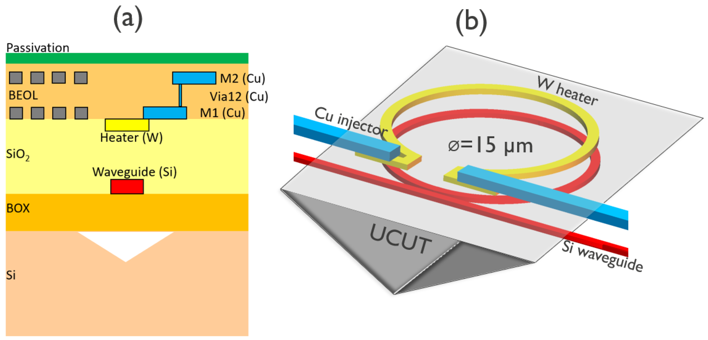
1.1. Silicon Photonic Heaters

Silicon photonics leverages decades of technological developments of classical CMOS processing to fabricate optical transceivers [4]. Silicon has many favorable optical properties, such as transparency in the telecom wavelength range and the plasma dispersion effect, which enables fast electro-optic actuation. Silicon also has a strong thermo-optic coefficient ($1.8·{10}^{-4}{K}^{-1}$), causing its refractive index to increase with temperature. This effect is much slower (µs) compared to electro-optic effects (ps), but also stronger, allowing for a wide range of phase controls in Si waveguides. Thermo-optic actuation is achieved with integrated heaters, which are typically metallic (W, TiN [5]) or doped Si [6]. Describing the time dynamics of a thermo-optic response in a SiPho device is important. For example, in interferometric devices (Mach–Zehnder-based, MZI [7]), heaters can be used to create a thermo-optic switch for optical routing and, in this case, a fast thermal response is preferred. Another example are ring heaters used in resonant devices such as ring modulators or filters. These heaters are used for thermal tuning (i.e., ring waveguide temperature control) such that the device’s resonance wavelength stays locked to the input light wavelength. Also for these devices, fast thermal response is preferred, such that the temperature control loop can actively stabilize the device temperature.

In the literature, there have been numerous studies reporting different heating and cooling time constants for SiPho devices. In Figure 1, a survey of published data for MZI time constants is shown. In some cases, it appears that heating is faster than cooling, but the opposite can also be true in other cases. The data are plotted for standard MZIs (Figure 1, left) and for devices with substrate undercut (i.e., UCUT) (Figure 1, right). UCUT is a design feature where part of the Si substrate is removed below the waveguide to improve the thermal isolation (Figure 2). None of the cited works provide an explanation as to where this hysteresis comes from. The objective of this paper is to explain the observations and provide a framework and guidelines for a more standardized way of doing thermo-optic characterization.

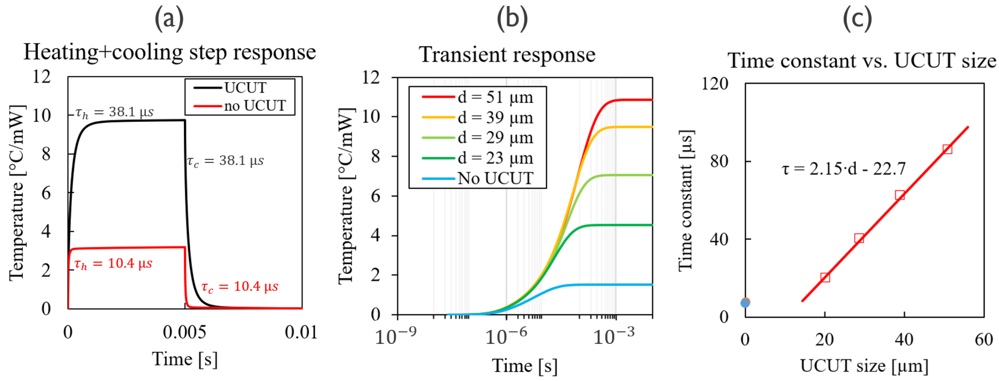
1.2. Heat Equation and Its Solution

Before starting any thermal simulations, we briefly study the analytical solution to the standard heat equation. This will provide valuable insight in the physics for later in the paper. The partial differential equation (PDE) that describes the rate of temperature change in a control volume is given by (adapted from [16]):

$$\frac{\partial T\left(t\right)}{\partial t}=\alpha \left(\frac{{\partial }^{2}T}{\partial x^2}+\frac{{\partial }^{2}T}{\partial y^2}+\frac{{\partial }^{2}T}{\partial z^2}\right)+\frac{\dot{q}}{c\rho }-\frac{hA}{c\rho V}(T-T_{\infty })$$

(1)

where $\alpha$ is the thermal diffusivity, $\dot{q}$ internal heat generation, c is the specific heat, $\rho$ is the density, h is the convective heat transfer coefficient, A is the convective cooling area, V is the volume and $T_{\infty }$ is the ambient temperature. Equation (1) is a more elaborate form of the basic first order ordinary differential equation, given by:

$$\tau \frac{dT\left(t\right)}{dt}+T\left(t\right)=f\left(t\right)$$

(2)

where $T\left(t\right)$ represents the heat transfer term (conduction and convection) and $f\left(t\right)$ is an externally applied term (e.g., heat generation). The time constant $\tau$ is related to the physical properties of the system:

$$\tau =\frac{\rho Vc}{hA}$$

(3)

The solution to Equation (2), given an initial condition $T_0$ and no external function $f\left(t\right)=0$ is:

$$T\left(t\right)=T_0{e}^{-t/\tau }$$

(4)

which describes the cooling response using an exponential temperature decay with time constant $\tau$. Now, for initial condition $T_0=0$, and with applied power ($f\left(0\right)\ne 0$), we obtain:

$$T\left(t\right)=f\left(0\right)\left(1-e^{-t/\tau }\right)$$

(5)

which describes the heating response to a power step function, with the same time constant $\tau$. Theoretically, the time constant for heating and cooling is identical in a linear, time invariant (LTI) system and determined by physical properties (Equation (3)). This means that the reported difference in heating and cooling times in the literature is a measurement artifact, caused by non-linearities in the system. This should, in fact, be avoided, as there currently is no consensus on how to report the thermo-optic time constants.

This paper is structured as follows: In Section 2 an in-depth analysis is performed for interferometric devices with linear heaters. In Section 3, the analysis is repeated for resonsant devices with ring heaters. In each section, first a theoretical description is given on the thermo-optic response, which is followed up by an analysis of the typical dynamic characterization methods. Here, we provide guidelines on how to perform characterization without non-linearities. Then, we also show how to convert measurement results that contain non-linearities into ’correct’ results, where the unwanted effects are filtered out.

2. Interferometric Devices

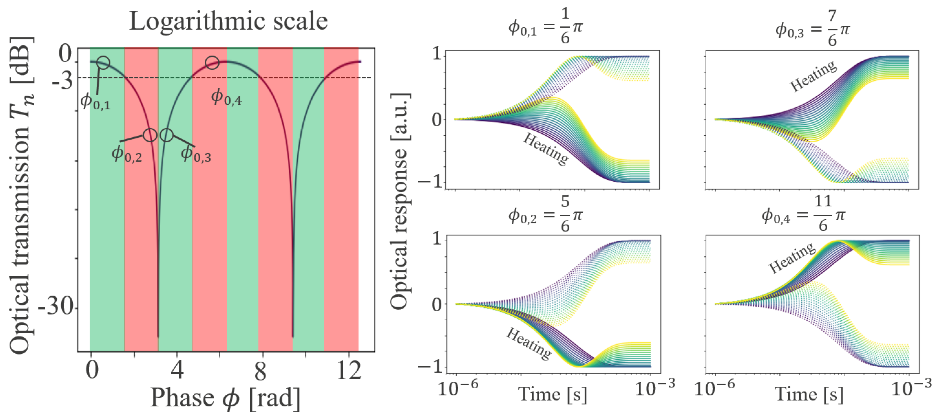
2.1. Theoretical Description

A schematic of one MZI arm with a thermo-optic phase shifter is shown in Figure 2A, and a Si photonic die cross-section is shown in Figure 2B, highlighting the thermal parts of interest: the Si waveguide (WG) where the light is contained, the W metallic heater (MHD), the substrate undercut (UCUT), and the insulation trench. The waveguide temperature $T\left(x\right)$ is linked to the optical phase shift $\varphi$ [13] which, in turn, determines the optical transmission $T_n$ of the MZI [17,18]:

$$\Delta \varphi ={\int }_0^L\frac{2\pi }{{\lambda }_0}\frac{d{n}_{eff}}{dT}\Delta T\left(x\right)dx$$

(6)

$$T_n\left(\varphi \right)=10·\log \left({\cos }^2(\varphi /2)\right)$$

(7)

where ${\lambda }_0$ is the light wavelength, L the device length and $d{n}_{eff}/dT$ the thermo-optic coefficient of the effective refractive index. The dynamic performance of the device, also referred to as a thermo-optic (TO) phase shifter, is characterized by applying a step function of heater power. From the analytical solution of the heat equation, it is known that the temperature response to such a step function is described by an exponential function:

$$\Delta T_{heating}\left(t\right)=R_{th,wg}·P_{th}·(1-e^{-t/{\tau }_{th}})$$

(8)

where $R_{th,wg}·P_{th}$ is the waveguide thermal resistance–power product, representing the steady-state temperature. Note that a realistic thermal step response will contain multiple time constants, each representing different parts of the die heating up sequentially. Here, we simplify the analysis and lump the dynamic response in a single time constant. When the steady-state is reached, the power can be switched off to cool down the waveguide again:

$$\Delta T_{cooling}\left(t\right)=R_{th,wg}·P_{th}·\left(e^{-t/{\tau }_{th}}\right)$$

(9)

Both analytical solutions contain the same time constant ${\tau }_{th}$. Hence, one would expect that ${\tau }_{th}={\tau }_{heating}={\tau }_{cooling}$, given that no thermal non-linearities are present, e.g., temperature-dependent thermal conductivity. However, in numerous other works, there have been reports of large discrepancies between heating and cooling time constants. The hypothesis is that the asymmetry between heating and cooling is caused by the non-linear optical transmission. The pure thermal time constant (as shown in Equations (8) and (9)) will be referred to as ${\tau }_{th}$, while the thermo-optic time constant will be referred to as ${\tau }_{TO}$. Note that in the literature, there exists no distinction between either metric.

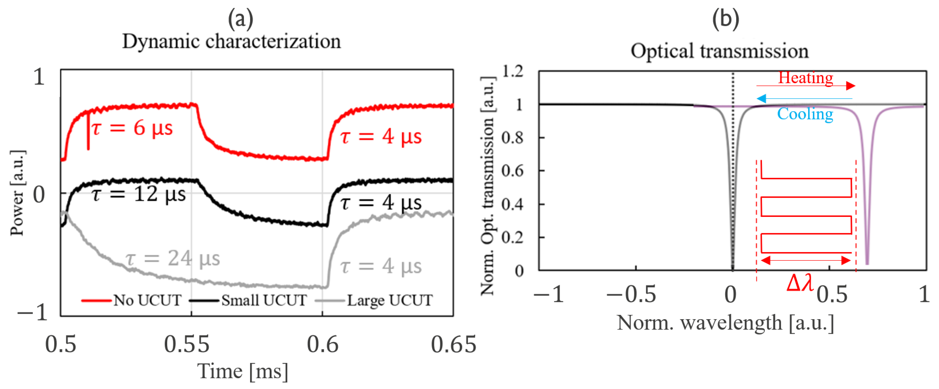
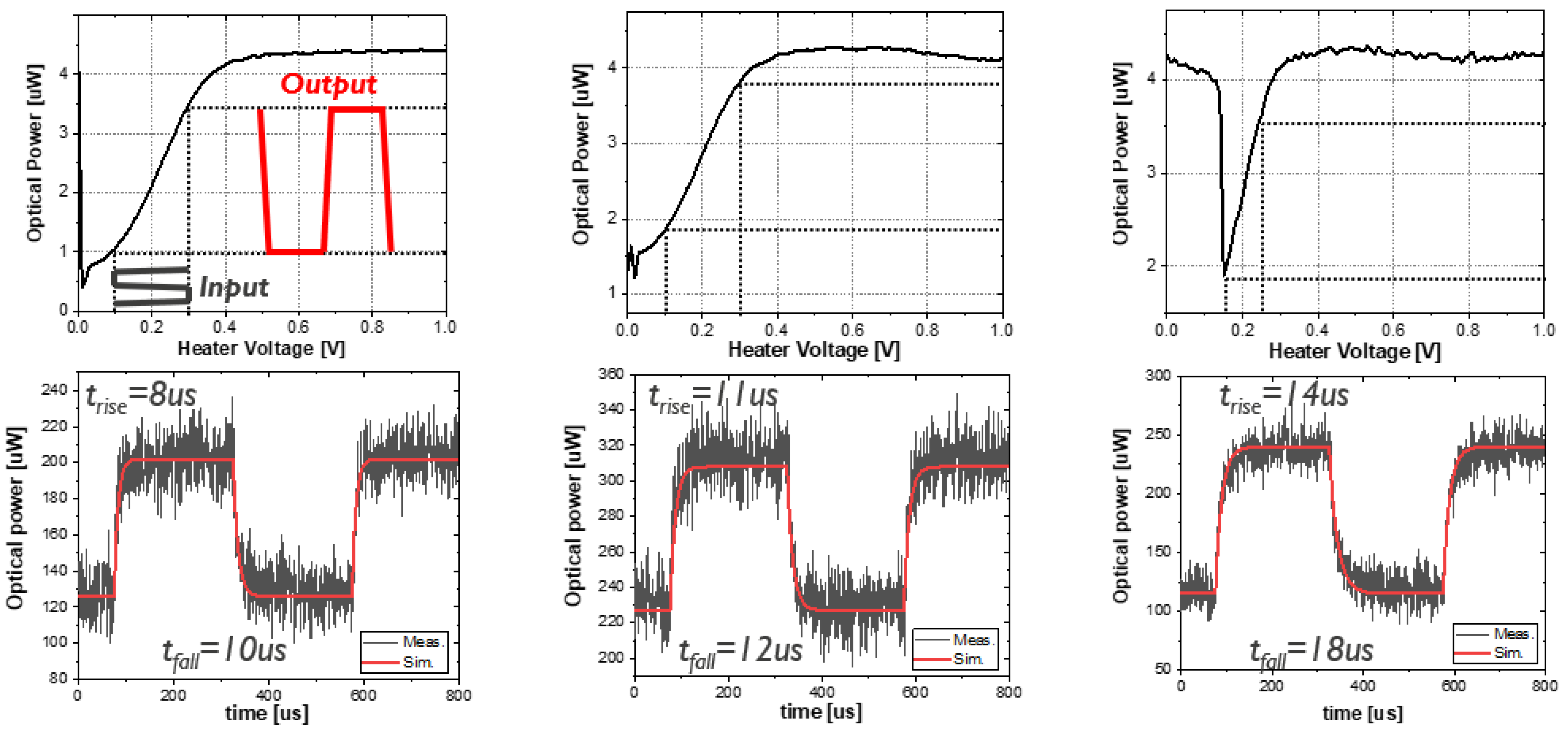
2.2. Dynamic Characterization Method

2.2.1. Analytical Model

The typical experimental procedure for extracting the thermo-optic time constant is explained using Figure 3. The optical transmission is shown on a logarithmic scale on the left, and on a linear scale on the right. First, a center point with phase ${\varphi }_0$ is chosen. In this example, ${\varphi }_0=3/2\pi$ is used, as it is exactly in the middle point of the optical transmission: $T_n(3/2\pi )=0.5$. A square wave of power is applied to the heater, which results in $\Delta \varphi$. The frequency of the square wave should be sufficiently low, such that thermal steady-state can be reached before each state transition. The optical response $\Delta T_n$ of the MZI is measured over time, and this time trace is used to calculate the thermal time constant, which is defined as the time required to reach $(1-1/e)\approx 0.63$ times the steady-state temperature.

The optical transmission during the heating (Equation (10)) and cooling (Equation (11)) step response can be simulated by adapting Equation (7) and filling in the center phase ${\varphi }_0$ and phase difference $\Delta \varphi$ between the on- and off-states:

$$T_n\left(t\right)={\cos }^2\left[\frac{({\varphi }_0-\Delta \varphi /2)+\Delta \varphi \left(t\right)}{2}\right]$$

(10)

$$T_n\left(t\right)={\cos }^2\left[\frac{({\varphi }_0+\Delta \varphi /2)-\Delta \varphi \left(t\right)}{2}\right]$$

(11)

In Equations (10) and (11) the time-dependent phase $\Delta \varphi \left(t\right)$ can be substituted using the expression for phase in Equation (6) in the function of temperature. Furthermore, the time-dependent temperature can be substituted by the steady-state temperature multiplied with an exponential time dependence (see Equation (8)). Combining all these results, the full expression of optical transmission in function of time and temperature is obtained:

$$T_n\left(T(x,t)\right)=10·\log \left({\cos }^2\left[\frac{({\varphi }_0-\Delta \varphi /2)+{\int }_0^L\frac{2\pi }{{\lambda }_0}\frac{d{n}_{eff}}{dT}T(x,t)dx·(1-e^{-t/\tau })}{2}\right]\right)$$

(12)

2.2.2. Impact of $\Delta \varphi$ and ${\varphi }_0$ on ${\tau }_{TO}$

The analytical dynamic thermo-optic model is used to simulate the impact of measurement conditions ${\varphi }_0$, $\Delta \varphi$ on the extracted time constant. To filter out optical non-linearities, small-signal analysis can be performed by choosing a small $\Delta \varphi$, and center phase ${\varphi }_0=3/2\pi$, with the goal of staying in the linear part of the optical transmission curve. The transient response to heating and cooling step functions is now simulated for $\pi /10<\Delta \varphi <\pi$, and the results are shown in Figure 4. Heating (a) and cooling (b) curves are symmetrical: they exhibit the same time constant. However, the time constant for the different curves is not the same. In Figure 4c, the simulated time constants are shown in function of $\Delta \varphi$: by increasing $\Delta \varphi$, the time constants decrease monotonously: ${\tau }_{TO}\propto {(\Delta \varphi )}^{-1}$. The difference between the pure thermal time constant ${\tau }_{th}$ and the thermo-optic time constant ${\tau }_{TO}$ is indicated as well (green, $ϵ$). This result highlights the importance of a small $\Delta \varphi$ during the experimental characterization, as the value of ${\tau }_{TO}$ converges to the value of ${\tau }_{th}$. Also, because the measurement result itself depends on the measurement conditions, it is of the utmost importance to report all properties of the applied square wave (frequency and amplitude) when discussing dynamic performance and time constants.

These results still do not provide an explanation for the asymmetry between heating and cooling reported in the literature. So, as a next step, ${\varphi }_0$ is swept between $3/2\pi <{\varphi }_0<9/5\pi$. The optical transmission is normalized and plotted in Figure 5 for two specific cases: ${\varphi }_0=3/2\pi$ (left) and ${\varphi }_0=9/5\pi$ (right). On the left figure, the aforementioned symmetry between heating and cooling is clearly illustrated (see results in Figure 4). Also, after normalizing the curves, it becomes apparent that the curves for different $\Delta \varphi$ do not coincide, hence their different time constants. The results in Figure 5 (right) show clear asymmetry between heating and cooling response, caused by the optical non-linearity in the transmission behavior close to ${\varphi }_0=9/5\pi$.

The time constants for heating and cooling are plotted in function of $\Delta \varphi$ with ${\varphi }_0$ as parameter in Figure 6. As we move away from the center phase ${\varphi }_0=3/2\pi$, more asymmetry between heating and cooling is introduced. To illustrate this, the difference in time constant $\Delta {\tau }_{TO}={\tau }_{heating}-{\tau }_{cooling}$ is shown in Figure 6 (right). The simulated cooling time constant is up to 200 µs larger compared to the heating time constant, validating the theory that the asymmetry between heating and cooling in the literature is caused by the optical non-linearity of the transmission.

The results in Figure 6 show that the measured cooling time constant can become larger than the heating time constant. However, from the literature review (Figure 1), it is also observed that, in some cases, the opposite is true. To investigate why this happens, simulations are performed for more values ${\varphi }_0$. The optical response is plotted in Figure 7 (right): the heating response is indicated with solid lines and the cooling response with dashed lines. Depending on the interval in which ${\varphi }_0$ is located, either heating or cooling can have a larger time constant. These interval are color-coded in Figure 7 (left), green intervals exhibit larger heating time constants. There is a periodicity of $\pi$ visible. The extracted time constants are plotted in Figure 8. At ${\varphi }_0=\pi /2+n\pi$, heating and cooling show identical time constants, at these points $T_n\left({\varphi }_0\right)=0.5$. At ${\varphi }_0=\pi$ the simulations reveal a discontinuity, so it is not advisable to use this value for characterization.

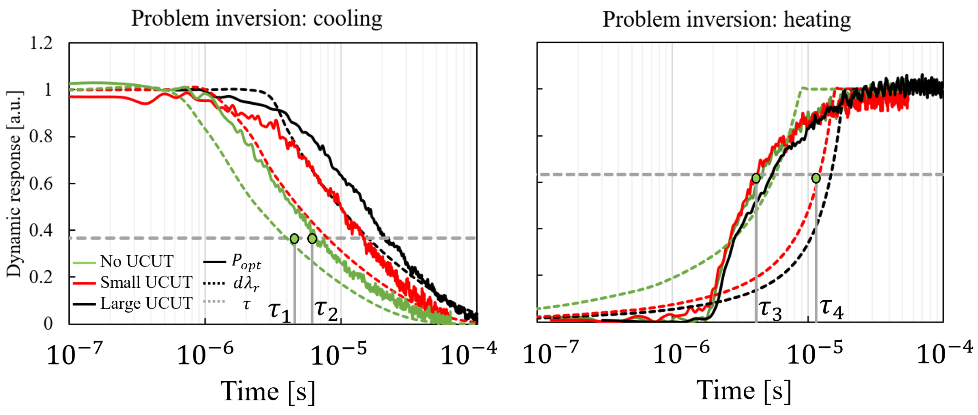
2.3. Problem Inversion

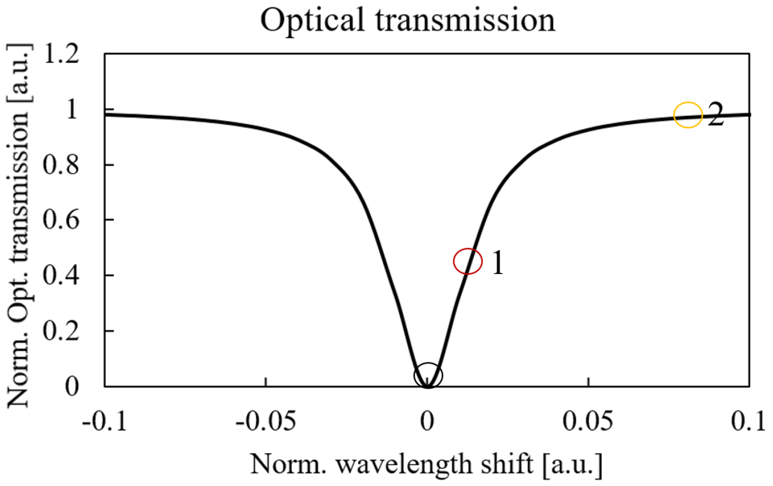
In the final part of the interferometric devices section, problem inversion is discussed. By this, we mean the following: The forward problem is, given ${\varphi }_0$ and $\Delta \varphi$, calculating the optical response $T_n\left(t\right)$. For the inverse problem, we take a measured or simulated $T_n\left(t\right)$, and try to extract the thermal time constant, even in the presence of optical non-linearity. This is useful, as it allows to reverse-engineer a thermal time constant from a ’bad’ set of measurements. Because the forward problem was solved using an analytical expression, the inverse problem is simply solved by taking Equation (7) and rewriting it in function of $\Delta \varphi \left(t\right)$:

$$\Delta \varphi \left(t\right)=2·\arccos \left(\sqrt{{10}^{T_n\left(t\right)/10}}\right)$$

(13)

Multiple heating optical transmission curves are simulated in Figure 9, for increasing non-linearity. The inverse model in Equation (13) is used to calculate the time dependent phase (which is directly proportional to waveguide temperature), and the results are shown as dashed lines. It is clear that independent of the choice of ${\varphi }_0$, the inverted thermal response remains constant.

3. Resonant Devices

In the second part of this work, we discuss the dynamic thermo-optic response for resonant devices. Ring modulators (RM) or ring wavelength filters fall under this category. These devices are ring-based to exploit optical resonance, and are equipped with an integrated ring heater to control the waveguide temperature and resonance wavelength. Accurately describing the thermo-optic time constant is important for the design of the thermal tuning controller. In the present study, we only consider heat generation in the integrated heater, and ignore any waveguide self-heating due to optical absorption. Any heat that originates from thermal crosstalk is also ignored. A typical SiPho die cross-section is shown in Figure 10a, and a basic ring modulator with ring heater in Figure 10b. The main difference with the interferometric devices from the previous section is the optical transmission function, which is based on a Lorentzian lineshape for resonant devices.

3.1. Theoretical Description

The analytical solution to the heat equation (Equations (4) and (5)) also applies here, meaning that the same time constant for heating and cooling is expected. This is verified numerically by conducting a transient finite element (FE) thermal simulation [19] of a heating step followed up by a cooling step in Figure 11a. More details on FE modeling is available in [20]. It is also observed that the introduction of UCUT causes a rise in thermal time constant. Furthermore, if the transient heating response is simulated for different UCUT sizes between 23 µm and 51 µm, a linear relationship between UCUT size and thermal time constant is obtained (Figure 11b,c). This can be explained by using the definition of the time constant (Equation (3)): $\tau \propto \rho Vc$; as the UCUT size increases, heat conduction is forced around the edges of the UCUT and more material is required to heat up before steady state is reached.

The aforementioned results showcase the pure thermal behavior. Now, the waveguide temperature has to be linked to the optical transmission. To model the optical transmission, a simplified form of the transmission function is proposed, based on a normalised Lorentzian lineshape [21] and a fitting parameter $\beta$, which is proportional to the ring Q factor [22].

$$P_{opt}\left(t\right)=1-\frac{1}{1+\beta {\left({\lambda }_r\left(t\right)\right)}^2}$$

(14)

The definition of the heater efficiency is used to relate waveguide temperature to resonance wavelength [20]:

$${\eta }_h=\frac{d\overline{T_{wg}}}{dP}=\frac{d\lambda }{dP}\frac{\lambda }{FSR·2\pi r·\frac{d{n}_{eff}}{dT}},$$

(15)

where $FSR$ is the free spectral range, $\lambda$ is the wavelength, r the RM radius and $d{n}_{eff}/dT=1.95·{10}^{-4}{K}^{-1}$ the thermo-optic coefficient of the effective refractive index for C-band wavelength (∼1.55 µm) for this modulator. The heater efficiency ${\eta }_h$ is either expressed in units of K/mW or pm/mW, and both figures of merit can be converted into each other using Equation (15). This equation also shows that there exists a linear relationship between waveguide temperature and resonance wavelength, which will be utilized later on. The resonance wavelength shift ${\lambda }_r\left(t\right)$ in Equation (14) is substituted with the expression for average waveguide temperature $\overline{T_{wg}}\left(t\right)$ (Equation (15)):

$$P_{opt}\left(t\right)=1-\frac{1}{1+\beta {\left(\overline{T_{wg}}\left(t\right)\times \left[\frac{FSR·2\pi \left(\frac{\partial n_{eff}}{\partial T}\right)}{\lambda }\right]\right)}^2}$$

(16)

With these expressions for optical power in function of waveguide temperature, both the heating and cooling response can be simulated by substituting $\overline{T_{wg}}\left(t\right)$ with a thermal step response obtain from FE simulation [20] (Figure 11). Because of the non-linear optical transmission, an optical hysteresis is introduced into the system. This hysteresis causes the heating and cooling curve to have a different time constant ${\tau }_{TO}$.

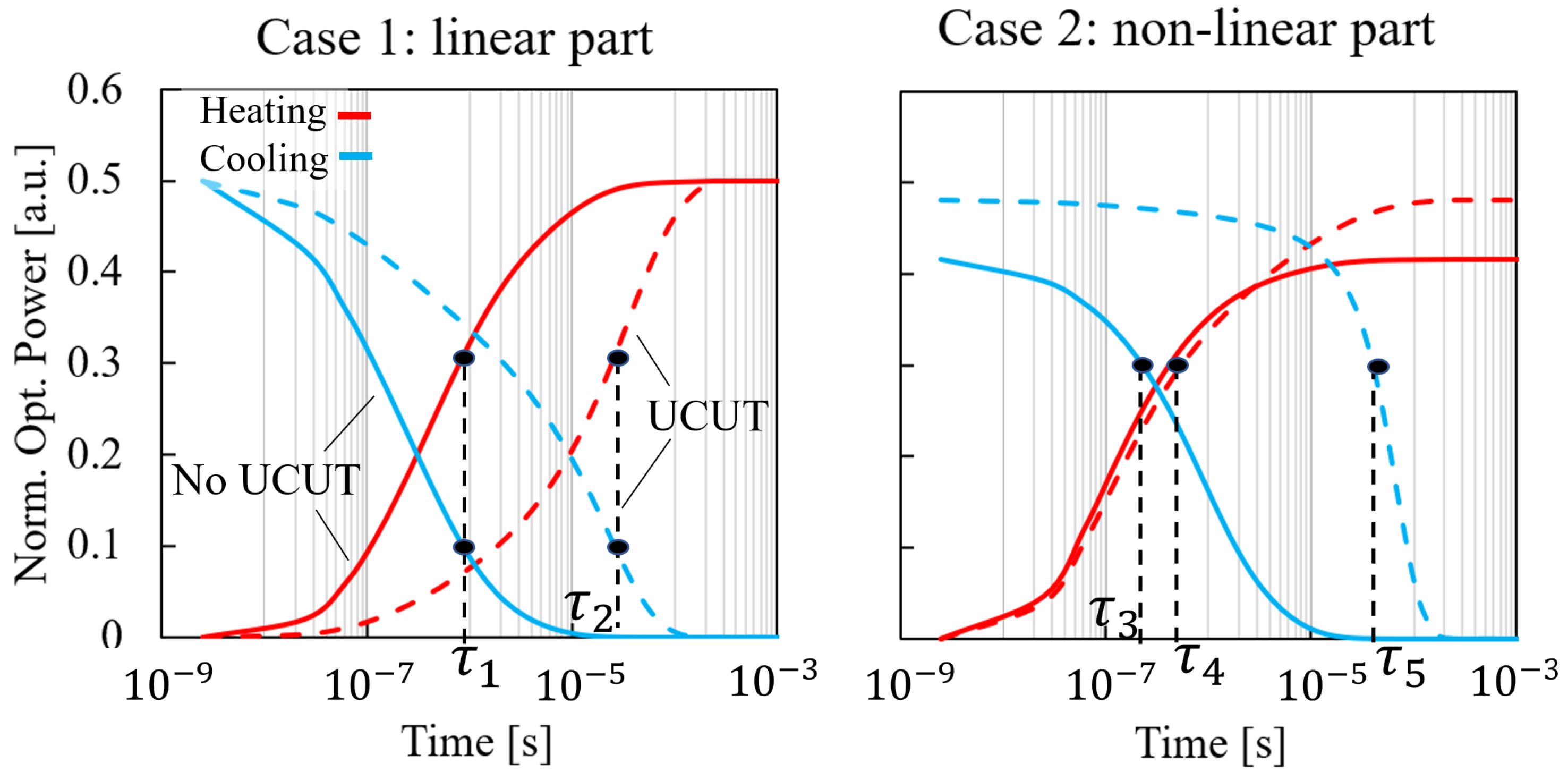
3.2. Dynamic Characterization Method

The dynamic characterization method for ring heaters is similar to the method used for the MZI heater. A square wave of heater power is applied, such that the device alternates between two states (unheated and heated), and the resulting optical transmission is measured. This concept is illustrated in Figure 12b. Given the positive thermo-optic coefficient, a temperature increase will result in a red-shift of the device resonance wavelength.

The measurement result in Figure 12a shows the optical transmission for a ring with and without UCUT. The vertical off-set between the curves can be ignored, as the measurement result is normalized and plotted such that the different curves are visible (not on top of each other). Interestingly, heating times stay the same for all cases. This is contrary to what is simulated in the previous section (Figure 11), where the UCUT clearly increased the thermal time constant of the waveguide. Furthermore, cooling time increases by the introduction of UCUT; the device with UCUT has a larger cooling time than heating time. Again, this is not in line with the simulated heating and cooling in Figure 11 which, theoretically, should have the same time constant. How is it possible that the experiments do not agree with the simulations?

In order to further explore the impact of the non-linear optical transmission, two different scenarios are compared through simulation. In Figure 13, the two scenarios are shown: for the first scenario, heating and cooling happens between state 0 and state 1. For the second scenario, this is between state 0 and state 2. The simulation results for both scenarios are shown in Figure 14. The first scenario shows that heating and cooling have the same time constant, and the time constant increases by the addition of UCUT. The reason for this behavior is that heating and cooling occurs inside the linear part of the transmission curve. The second scenario falls outside the linear part. This results in different time constants for heating and cooling: in Figure 14, ${\tau }_4\ne {\tau }_5$ and furthermore because of the optical non-linearity, it appears that the heating time constant is identical with and without UCUT. The simulated time constants are summarized in

Table 1. Simulated thermal time constants ${\tau }_{TO}$ [µs] for two cases (Figure 14) with model of ring modulator.

	Case 1		Case 2
	Heating	Cooling	Heating	Cooling
No UCUT	6	6	0.3	4.8
UCUT	28	28	0.6	66.2

. Due to the optical non-linearity, it appears that cooling is slower. Intuitively, this can be understood by inspecting the optical transmission curve (Figure 14): when cooling down, the transmission shifts from point (2) to (0), where the fast initial thermal response mainly covers the flat part of the transmission curve, so it appears that the device response is delayed. Only close to the steady-state is there a sudden drop in optical transmission at the resonance peak. For the heating response, the opposite is true when moving from point (0) to (2).

It is beneficial to stay within the (approximately) linear part of the optical transmission when doing the characterization. This way, the experimental result can directly be compared with simulation results. A criterion for staying in the linear regime (Figure 13, 0–1) is that the wavelength shift from resonance should be smaller than 50% full width at half maximum (FWHM). This is explained using Figure 15: FWHM/2 overlaps with the linear part (gray zone) of the transmission curve (black). The derivative of the transmission is also shown in red: in the gray zone, the derivative is approximately constant. Because the ring modulator FWHM is related to its quality factor according to $FWHM={\lambda }_{res}/Q_{fac}$, the allowed heater power that can be used during the characterization in order to stay in the linear regime is:

$$P_{heater}<\frac{2{\lambda }_{res}}{Q_{fac}{\eta }_h}$$

(17)

with ${\eta }_h$ being the heater efficiency in units of nm/mW. This rule of thumb is applied, and the ring modulators are characterized experimentally. The result is shown in Figure 16, for devices without UCUT (left), small UCUT (16 × 24 µm², middle) and large UCUT (34 × 34 µm², right). By limiting the applied voltage to the heater, operation within the linear regime is ensured. Note that the heater voltage step is decreased from 0.2 V to 0.1 V for the large UCUT case, because of the increased heater efficiency. The results now show what is theoretically predicted in Figure 10: a larger UCUT size corresponds to larger time constants. Furthermore, heating and cooling time constants are the same (within the accuracy limits of the measurement).

3.3. Problem Inversion

Using the model proposed in Equation (16), the forward problem is solved: a simulated waveguide temperature can be converted into an optical power change at the device output. This is useful for comparing simulations with experimental results, which show signs of optical hysteresis or non-linearity. Furthermore, experimental characterization according to the described method is fast and efficient: the experiment is only performed for a single wavelength.

As a next step, the inverse problem is solved. Can a measured optical response containing hysteresis (${\tau }_{TO}$), such as the one in Figure 12, be converted to waveguide temperature or equivalent resonance wavelength (${\tau }_{th}$)? To solve this, the model in Equation (16) is written in function of ${\lambda }_r$:

$${\lambda }_{r,heating}\left(t\right)=\sqrt{\frac{1}{\beta }\left(\frac{1}{1-P_{opt}\left(t\right)}-1\right)}$$

(18)

To simplify the equations, they are written in terms of the function of resonance wavelength (instead of the waveguide temperature). The results are shown in Figure 17. The experimental results (from Figure 12) are shown in solid lines: they are obtained by doing characterization outside the linear regime of the optical transmission. The dotted lines show the simulation according to the model in Equation (18): for cooling, the time constants are overestimated by the measurements ${\tau }_{2,TO}>{\tau }_{1,th}$, while for heating, the opposite is true ${\tau }_{3,TO}<{\tau }_{4,th}$. These simulated time constants (

Table 2. Time constants ${\tau }_{TO}$ extracted from the profiles in Figure 17. The experiments are carried out outside of linear regime, but can still be converted using the inverse model (Equation (18)) to obtain time constants ${\tau }_{th}$ [µs], which are in line with the predicted results from FE simulation.

	Cooling		Heating
	Exp. ${\mathit{\tau }}_{\mathit{TO}}$	Converted ${\mathit{\tau }}_{\mathit{th}}$	Exp. ${\mathit{\tau }}_{\mathit{TO}}$	Converted ${\mathit{\tau }}_{\mathit{th}}$
No UCUT	6	5	4	5
Small UCUT	12	9	4	9
Large UCUT	24	18	4	18

), derived from experiments with hysteresis, are in good agreement with the experimental results without hysteresis (Figure 16).

3.4. Alternative Dynamic Characterization Method

To conclude the discussion on the thermo-optic time constant in resonant devices, we propose an alternative characterization method. Instead of measuring the optical transmission (which can contain non-linear effects), we propose to measure the change in resonance wavelength, which is linearly proportional to waveguide temperature (Equation (15)).

The experimental method is explained using the measurement result in Figure 18: the ring transmission is red-shifted after application of a heater step function (black to purple in Figure 18, bottom). The input wavelength of the light is chosen to be between the start and end resonance wavelength of the ring. As the ring resonance passes by the light input wavelength during heating, one optical power trace is obtained for this specific wavelength. The shape of the curves can be explained as follows: we are effectively measuring a convolution of the ring transmission spectrum (Lorentzian) and an exponential waveguide temperature increase. The wavelengths (colors) in Figure 18, which are close to the idle ring resonance are passed quickly (<1 µs), resulting in a sharp optical power trace. The wavelengths that are a further distance away are passed when the ring is close to thermal steady state, which occurs much slower (<10 µs). This optical power trace is shown in Figure 18 (top). From the optical power trace, the time required for reaching the new resonance wavelength can be extracted. Combined with the wavelength mismatch between the input light and original ring resonance, the time evolution of the resonance wavelength is found. This measurement is repeated for multiple input wavelengths (different colors in Figure 18). To calibrate the FE model, it is suggested to measure at least ten different wavelengths to obtain sufficient resolution in the extracted wavelength shift over time. In our experiment, a 10 mW heater power step is applied, which corresponds to an approximately 2.5 nm wavelength shift. This 2.5 nm is divided in 10 steps of 250 pm, and this results in a smooth curve of wavelength vs. time. The most important drawback of this type of experimental characterization is the larger number of required measurements for the extraction of a single time constant. The main benefit, however, is that the pure thermal time constant is obtained, which is unaffected by the non-linear optical transmission.

4. Discussion

The results for both interferometric and resonant devices show that the extracted thermo-optic time constant depends on the settings of the characterization experiment. The proposed models allow us to interpret any variations that are measured, for example a different heating and cooling time constant within the same device. One aspect that was not touched upon is device-to-device variability. Wafer-level intrinsic or extrinsic variations in material properties can cause a difference in dynamic thermal responses [23]. For example, the heat capacity of Si can vary across the wafer which, in turn, influences the thermal time constant. This analysis is left for future work. In this work, we focused on the optical non-linearities of the photonic devices. There also exist different types of non-linearities: thermal non-linearity is caused by the temperature dependent thermal conductivity of the material. As silicon’s thermal conductivity decreases with temperature, a different thermal time constant will be obtained at room temperature vs. at 100 °C. Electrical non-linearity can also impact the measurement result: the metallic heaters exhibit a positive temperature coefficient of resistance (TCR). At elevated temperatures, the electrical resistance will be increased, resulting in more Joule heat dissipation for the same current. This can be counteracted by monitoring both heater voltage and current, and carrying out the experiment at constant power condition.

The MZI is analyzed theoretically; we did not present any new measurement data that validates our claims. However, the numerical simulations agree well with analytical predictions using the heat equation. The outlook for this device research is to replicate the theoretical results from Figure 4 and Figure 5 experimentally, such that the difference between heating and cooling time constant can be documented. For the ring modulator, we present a theoretical model and experimental data that validates the model.

5. Conclusions

In the literature, there exist ambiguity on how to measure and report thermo-optic time constants in silicon photonic devices. In this paper, we propose guidelines for the dynamic thermo-optic characterization of such devices. The analysis is performed for a Mach–Zehnder interferometer (MZI) and a ring modulator. If these guidelines are not followed, the obtained thermo-optic time constant for heating and cooling can be significantly different. For MZIs, the characterization is to be performed at ${\varphi }_0=\pi /2+n\pi$, such that balanced transmission is achieved ($T_n\left({\varphi }_0\right)=0.5$), and the applied phase shift $\Delta \varphi <\pi /10$ has to be sufficiently small. This ensures a linear optical transmission response. For the dynamic characterization of the ring modulator, we show experimentally that the obtained thermo-optic time constant greatly varies depending on the settings of the experiment. A maximum allowed heater power to remain in the linear part of the optical transmission is derived based on device metrics ($P_{heater}<2{\lambda }_{res}/\left(Q_{fac}{\eta }_h\right)$). Finally, an alternative method for characterization is proposed for the ring modulator where the temporal evolution of the ring resonance wavelength is tracked. This is useful, as it is directly proportional to waveguide temperature, and this type of measurement can be used to extract a pure thermal time constant.

References

1. Rakowski, M.; Ban, Y.; De Heyn, P.; Pantano, N.; Snyder, B.; Balakrishnan, S.; Van Huylenbroeck, S.; Bogaerts, L.; Demeurisse, C.; Inoue, F.; et al. Hybrid 14 nm FinFET–Silicon Photonics Technology for Low-Power Tb/s/mm2 Optical I/O. In Proceedings of the 2018 IEEE Symposium on VLSI Technology, Honolulu, HI, USA, 18–22 June 2018. [Google Scholar]
2. Coenen, D.; Kim, M.; Oprins, H.; Ban, Y.; Velenis, D.; Van Campenhout, J.; De Wolf, I. Thermal Impact of 3D Hybrid Photonic-Electronic Integration on Ring Modulators. SPIE J. Opt. Microsyst. 2024, 4, 011004. [Google Scholar]
3. Nagarajan, R.; Ding, L.; Coccioli, R.; Kato, M.; Tan, R.; Tumne, P.; Patterson, M.; Liu, L. 2.5D Heterogeneous Integration for Silicon Photonics Engines in Optical Transceivers. IEEE J. Sel. Top. Quantum Electron. 2023, 29, 8200209. [Google Scholar] [CrossRef]
4. Ferraro, F.J.; De Heyn, P.; Kim, M.; Rajasekaran, N.; Berciano, M.; Muliuk, G.; Bode, D.; Lepage, G.; Janssen, S.; Magdziak, R.; et al. Imec silicon photonics platforms: Performance overview and roadmap. In Proceedings of the SPIE 12429, Next-Generation Optical Communication: Components, Sub-Systems, and Systems XII, San Francisco, CA, USA, 31 January–2 February 2023. [Google Scholar]
5. Masood, A.; Pantouvaki, M.; Goossens, D.; Lepage, G.; Verheyen, P.; Van Thourhout, D.; Absil, P.; Bogaerts, W. CMOS-compatible Tungsten heaters for silicon photonic waveguides. In Proceedings of the 9th International Conference on Group IV Photonics, San Diego, CA, USA, 29–31 August 2012. [Google Scholar]
6. Masood, A.; Pantouvaki, M.; Lepage, G.; Verheyen, P.; Van Campenhout, J.; Absil, P.; Van Thourhout, D.; Bogaerts, W. Comparison of heater architectures for thermal control of silicon photonic circuits. In Proceedings of the 10th International Conference on Group IV Photonics, Seoul, Republic of Korea, 28–30 August 2013. [Google Scholar]
7. Dourado, D.M.; Rocha, M.L.; Carmo, J.P.P. Mach-Zehnder modulator modeling based on imec-ePixFab ISIPP25G SiPhotonics. In Proceedings of the 2018 SBFoton International Optics and Photonics Conference (SBFoton IOPC), Campinas, Brazil, 8–10 October 2018. [Google Scholar]
8. Liu, S.; Tian, Y.; Lu, Y.; Feng, J. Comparison of thermos-optic phase-shifters implemented on CUMEC silicon photonics platform. In Proceedings of the Seventh Symposium on Novel Photoelectronic Detection Technology and Application, Kunming, China, 5–7 November 2020. [Google Scholar]
9. Fang, Q.; Song, J.F.; Liow, T.Y.; Cai, H.; Yu, M.B.; Lo, G.Q.; Kwong, D.L. Ultralow power silicon photonics thermo-optic switch with suspended phase arms. IEEE Photonics Technol. Lett. 2011, 23, 525–527. [Google Scholar] [CrossRef]
10. Lu, Z.; Murray, K.; Jayatilleka, H.; Chrostowski, L. Michelson inter ferometer thermo-optic switch on SOI with a 50-uW power consumption. In Proceedings of the 2016 IEEE Photonics Conference (IPC), Waikoloa, HI, USA, 2–6 October 2016. [Google Scholar]
11. Celo, D.; Goodwill, D.J.; Jiang, J.; Dumais, P.; Li, M.; Bernier, E. Thermo-optic silicon photonics with low power and extreme resilience to over-drive. In Proceedings of the 2016 IEEE Optical Interconnects Conference (OI), San Diego, CA, USA, 9–11 May 2016. [Google Scholar]
12. Murray, K.; Lu, Z.; Jayatilleka, H.; Chrostowski, L. Dense dissimilar waveguide routing for highly efficient thermo-optic switches on silicon. Opt. Express 2015, 23, 19575–19585. [Google Scholar] [CrossRef] [PubMed]
13. Liu, S.; Feng, J.; Tian, Y.; Zhao, H.; Jin, L.; Ouyang, B.; Zhu, J.; Guo, J. Thermo-optic phase shifters based on silicon-on-insulator platform: State-of-the-art and a review. Front. Optoelectron. 2022, 15, 9. [Google Scholar] [CrossRef] [PubMed]
14. Yue, W.; Cai, Y.; Yu, M. Review of 2 × 2 Silicon Photonic Switches. Photonics 2023, 10, 564. [Google Scholar] [CrossRef]
15. Tong, W.; Wei, Y.; Zhou, H.; Dong, J.; Zhang, X. The Design of a Low-Loss, Fast-Response, Metal Thermo-Optic Phase Shifter Based on Coupled-Mode Theory. Photonics 2022, 9, 447. [Google Scholar] [CrossRef]
16. Cengel, Y.A.; Ghajar, A.J. Heat and Mass Transfer, 5th ed.; Mc Graw Hill: New York, NY, USA, 2015; pp. 74–237. [Google Scholar]
17. Ducournau, G.; Latry, O.; Ketata, M. The All-fiber MZI Structure for Optical DPSK Demodulation and Optical PSBT Encoding. Syst. Inform. 2013, 4, 79–89. [Google Scholar]
18. Coenen, D.; Kim, M.; Oprins, H.; Croes, K.; De Heyn, P.; Van Campenhout, J.; De Wolf, I. Static and Dynamic Thermal Modelling of Si Photonic Thermo-Optic Phase Shifter. In Proceedings of the 2024 23rd IEEE Intersociety Conference on Thermal and Thermomechanical Phenomena in Electronic Systems (iTherm), Denver, CO, USA, 28–31 May 2023. [Google Scholar]
19. MSC Software Corporation, Marc: Advanced Nonlinear Simulation Solution. Available online: https://www.mscsoftware.com/product/marc (accessed on 4 May 2022).
20. Coenen, D.; Oprins, H.; Ban, Y.; Ferraro, F.; Pantouvaki, M.; Van Campenhout, J.; De Wolf, I. Thermal modelling of Silicon Photonic Ring Modulator with Substrate Undercut. IEEE J. Lightwave Technol. 2022, 40, 4357–4363. [Google Scholar] [CrossRef]
21. Bogaerts, W.; De Heyn, P.; Van Vaerenbergh, T.; De Vos, K.; Kumar Selvaraja, S.; Claes, T.; Dumon, P.; Bienstman, P.; Van Thourhout, D.; Baets, R. Silicon microring resonators. Laser Photonics Rev. 2012, 6, 47–73. [Google Scholar] [CrossRef]
22. Coenen, D.; Kim, M.; Oprins, H.; Van Campenhout, J.; De Wolf, I. Coupled Dynamic Thermo-Optical Analysis and Compact Modelling of Self-Heating in Ring Modulator. In Proceedings of the 2023 International Conference on Photonics in Switching and Computing (PSC), Mantova, Italy, 26–29 September 2023. [Google Scholar]
23. Martinez-Hernandez, H.D.; Martinez-Munoz, P.E.; Ramirez-Gutierrez, C.F.; Martinez-Ascencio, E.U.; Millan-Malo, B.M.; Rodriguez-Garcia, M.E. Effect of Intrinsic and Extrinsic Defects on the Structural, Thermal, and Electrical Properties in p-Type CZ-Si Wafers with Different Carrier Concentrations. Int. J. Thermophys. 2022, 43, 181. [Google Scholar] [CrossRef]
Figure 1. The literature data for SiPho thermo-optic phase shifters without UCUT (left) and with UCUT (right). Orange data shows the heating time constant, and blue data shows the cooling time constant. A. Masood [6], S. Liu [8], Q. Fang [9], Z. Lu [10], D. Celo [11], K. Murray [12]. More examples are available in [13,14,15].
Photonics 11 00603 g001
Figure 2. (A) Sketch of waveguide with electro/thermo-optic modulation, and substrate undercut (UCUT). (B) shows the cross-section of the Si photonic die, with the thermal parts of interest: metal heater (MHD), Si waveguide (WG), UCUT and trench.
Photonics 11 00603 g002
Figure 3. Left: MZI transmission T n on a logarithmic scale. Right: transmission on a linear scale, zoomed-in between ϕ = π and ϕ = 2 π . The input for the thermal characterization is the applied square wave Δ ϕ power to the heater, which is centered around ϕ 0 . The resulting transmission Δ T n is measured optically.
Photonics 11 00603 g003
Figure 4. Simulated transient optical transmission with the model in Equation (12), for ϕ 0 = 3 / 2 π and Δ ϕ = [ π / 10 : 10 : π ] . (a) Heating response and (b) cooling response. (c) Extracted thermo-optic time constant τ T O and pure thermal time constant τ t h .
Photonics 11 00603 g004
Figure 5. Simulated transient optical transmission with the model in Equation (12), for ϕ 0 = 3 / 2 π (left) and ϕ 0 = 9 / 5 π (right) and Δ ϕ = [ π / 10 : 10 : π ] . The amplitude of the optical response is normalized. The results on the left show symmetry between heating and cooling, while the right results show asymmetry.
Photonics 11 00603 g005
Figure 6. Simulated time constants τ T O of optical transmission with the model in Equation (12), in function of Δ ϕ , with ϕ 0 = [ 3 / 2 π : 10 : 9 / 5 π ] as parameter. Left: heating response; middle: cooling. By increasing Δ ϕ and moving ϕ 0 towards 2 π , increasing levels of asymmetry are introduced. This is visualized in the right figure, which shows the difference between heating and cooling Δ τ T O = τ h e a t i n g τ c o o l i n g . For reference, the pure thermal time constant τ t h is also plotted (red).
Photonics 11 00603 g006
Figure 7. Left: optical transmission. The color code is used to indicate which time constant is the largest: in the red interval, cooling is the slowest; in the green interval, heating is the slowest. Four ϕ 0 points are indicated, and the transient optical response at these points for π / 20 < Δ ϕ < π / 2 is simulated (right). Solid lines are the heating response, dashed lines the cooling response.
Photonics 11 00603 g007
Figure 8. Simulated time constant for heating (solid) and cooling (dashed). In the green interval, heating is slower than cooling, and vice versa in the red interval.
Photonics 11 00603 g008
Figure 9. Simulated optical response (solid) for ϕ 0 = [ 1.8 π , 1.85 π , 1.9 π ] , for π / 20 < Δ ϕ < π / 2 , plotted for the left y-axis. The dashed lines represent the MZI phase Δ ϕ ( t ) , calculated with the inverted model in Equation (13), plotted for the right y-axis.
Photonics 11 00603 g009
Figure 10. (a) SiPho die cross-section. (b) Model geometry: ring heater, waveguide and UCUT are highlighted.
Photonics 11 00603 g010
Figure 11. (a) FE simulation of ring modulator heating and cooling response to a step function in linear time scale. Simulation shows identical rise and fall time τ t h . Addition of UCUT increases time constants. (b) Transient heating response (logarithmic time scale) for increasing UCUT size. (c) Extracted thermal time constants in function of UCUT size.
Photonics 11 00603 g011
Figure 12. (a) Dynamic measurement of optical response of ring modulator to a square wave heater power with 10 kHz frequency, without UCUT (red), with small UCUT (black) and large UCUT (grey, 5 kHz square wave is used in this measurement because cooling time did not reach steady state with 10 kHz heater frequency). Indicated time constants are thermo-optic τ T O . (b) Illustration of the unheated (black) and heated (purple) ring transmission spectrum, and the input wavelength (dotted line).
Photonics 11 00603 g012
Figure 13. Two different scenarios: heating and cooling between 0 and 1, and between 0 and 2.
Photonics 11 00603 g013
Figure 14. All indicated time constants are thermo-optic τ T O . Left: simulation (Equation (16)) of case 1 (Figure 13): inside the linear part of the transmission curve heating and cooling have the same time constants. Right: simulation of case 2: heating and cooling have different time constants ( τ 4 τ 5 ) and heating curves coincide; numerical results in Table 1. For case 1, τ 1 and τ 2 are the same for heating and cooling.
Photonics 11 00603 g014
Figure 15. Normalized ring modulator optical transmission (black) and its derivative with respect to wavelength (red). Full width half maximum (FWHM, green) is indicated, which matches well with the linear part of the spectrum, i.e., at constant derivative.
Photonics 11 00603 g015
Figure 16. Top: dynamic characterization inside linear regime of the optical transmission curve, heater voltage (x-axis) is limited < 0.3 V. Bottom: measured optical response (black) and model fit (red). Device without UCUT (left), small UCUT (16 × 24 µm2, middle) and large UCUT (34 × 34 µm2, right).
Photonics 11 00603 g016
Figure 17. Solid: measured optical power (Figure 12) outside of device linear regime. Dashed: simulated resonance wavelength shift with the inverse model in Equation (18). For cooling (left), the time constants are overestimated with the measurements: τ 2 , T O > τ 1 , t h . For heating (right), the time constants are underestimated: τ 3 , T O < τ 4 , t h , numerical results in Table 2.
Photonics 11 00603 g017
Figure 18. Dynamic measurement of resonance wavelength. Top: measured optical power over time after applying a heater power step function, for different input wavelengths which are progressively further from the ring resonance wavelength. Bottom: normalized optical transmission of ring modulator (black) and after applying a heater power step function (purple). Dotted lines correspond to experiments at different wavelengths.
Photonics 11 00603 g018