Fast 2D Subpixel Displacement Estimation

Abstract

Fast and simple methods for motion estimation with subpixel accuracy are of interest in a variety of applications. In this paper, we extend a recently proposed method for quantifying 1D displacements with subpixel accuracy, referred to as the subtraction method (SM) to 2D motion. Simulation and experimental results are presented. The results indicate that any general motion in 2D involving combinations of in-plane motions in x and y can be determined using SM after a 1D calibration. The errors between the actual motion and estimated are examined.

1. Introduction

Subpixel displacement estimation is a technique used in various fields to measure the shifts or movements of an object at a scale smaller than the pixel resolution of an imaging sensor, based on the images taken before and after the translation. Its importance spans several areas due to its capability to provide higher accuracy and finer details than standard pixel-level methods. For instance, subpixel methods enhance the capability to detect and analyze subtle motions, leading to a better performance in tracking and monitoring systems [1,2]. It also improves the analysis of satellite and aerial images by providing more precise data on land use, environmental changes, and urban development. Other applications include video compression [3], image stabilization [4], super-resolution imaging [5], and computer vision [6].

At present, such displacements are commonly determined using the correlation of images before and after the motion; we will refer to the correlation method (CM). Frequency-based correlation is considered more accurate and faster than commonly used spatial correlation methods such as normalized cross-correlation. The principles and algorithms used in digital image correlation for this application of in-plane displacement (along with strain measurement) have been described in [7,8]. The importance of CM is such that there is an extensive literature devoted to reducing the CM calculation time, increasing the lateral resolution, reducing peak-locking bias error and suppressing noise effects in digital images [9,10,11,12,13,14]. Other non-correlation-based techniques have been used to determine displacement, such as gradient-based methods [15] by analyzing the intensity gradients in the image, block matching [16] by dividing the image into blocks and finding the best match for each block in the next frame, phase-based techniques [2,17] by the use of phase gradients or phase unwrapping methods, analyzing the phase information of signals to estimate displacement, and pattern recognition techniques [18] by leveraging machine learning or deep learning models trained to recognize and predict displacement patterns based on image data. Each of these techniques has its advantages and is suitable for different applications, depending on factors like computational efficiency, robustness to noise and the specific characteristics of the displacement being measured.

We have previously introduced a novel fast approach, the subtraction method (SM), to estimate displacement [8,19,20] which only employs subtraction and addition operations. This algorithm is much faster than CM. One-dimensional motion measurement has been demonstrated in detail using both simulated and experimental data. Detailed comparisons of CM results to the corresponding SM results are also reported. In [21], Belen et al. performed an experiment with a portable photo booth having lead stripes and reflective walls. Hence, they demonstrated the capabilities of the SM to track subpixel displacements. They compared it with an interpolated cross-correlation function. Four different targets with displacements of 0.002 pixels were used, which they claim approaches the theoretical digital resolution limit. They demonstrate that SM can be used for motion estimation without suffering from peak-locking error, and thus is a reliable alternative to the correlation method.

In this paper, SM is analyzed and applied to 2D motion estimation using both simulated and experimental data for the first time. This is a non-trivial extension because of crosstalk between the two dimensions. We present simulation and experimental results that demonstrate how SM can be used to determine 2D motion following appropriate 1D calibration.

This paper is organized as follows: In Section 2, a 2D analysis of SM, using continuous and discrete functions, is presented. In Section 3, simulation results are used to examine in detail the relationship between 2D in-plane motion and the corresponding 1D components (in x and y) of that motion. In Section 4, illustrative experimental results are presented, and the errors examined. Finally, we present our conclusions.

2. Two-Dimensional Theory

In this section, we derive the theoretical model of SM for 2D motion. In Section 2.1 of [1], a theoretical analysis of SM for 1D motion was presented based on the Taylor series expansion, and we follow that presentation. It is also possible to derive the algorithm using Newton’s difference quotient or by interpreting it as a digital filter [20], but we omit those for space considerations. We consider the case of a continuous image in Section 2.1 and a discrete image in Section 2.2.

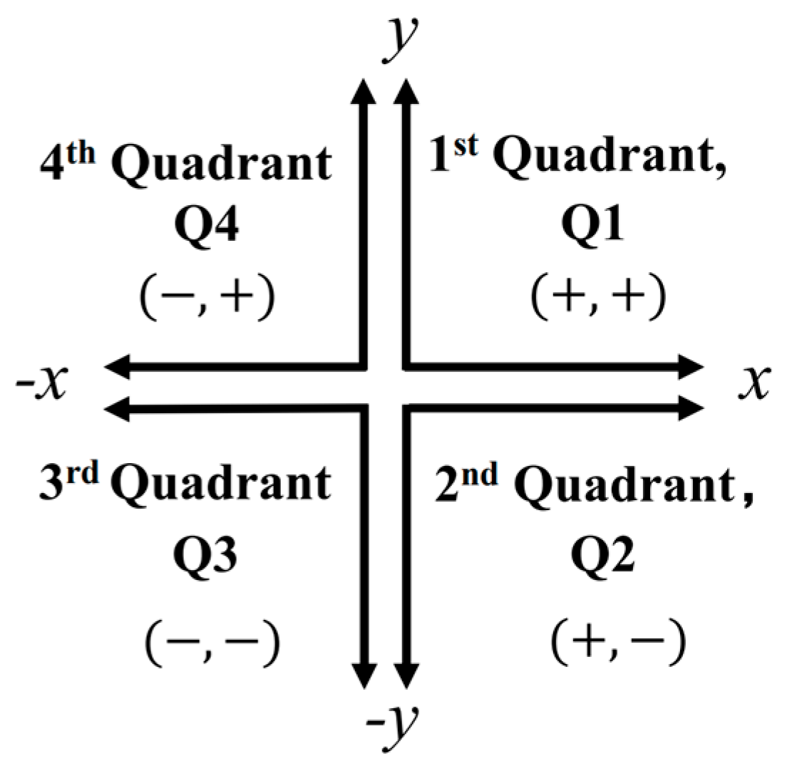
2.1. Continuous Model 2D Motion

Given an image, $I(x,y)$, over a given region, $a\le x\le b$, $c\le y\le d$, we expand $\left(x+∆x,y+∆y\right)$ around (x, y) using a Taylor series expansion.

$$I\left(x+∆x,y+∆y\right)=I\left(x,y\right)+I_x\left(x,y\right)∆x+I_y\left(x,y\right)∆y+R_{2,N},$$

(1)

We assume that higher-order terms are negligible, i.e., the remainder $R_{2,N}\approx 0$.

Let $I_x\left(x,y\right)$ and $I_y\left(x,y\right)$ be the partial derivatives of $I\left(x,y\right)$ with respect to x and y,

$$I_x\left(x,y\right)=\frac{\partial I\left(x,y\right)}{\partial x},\hspace{1em}\hspace{1em}\hspace{1em}\hspace{1em}{I}_y\left(x,y\right)=\frac{\partial I\left(x,y\right)}{\partial y}.$$

(2)

We now define a difference function between the original image and the translated image.

$$D\left(x,y;∆x,∆y\right)=I\left(x+∆x,y+∆y\right)-I\left(x,y\right)\approx I_x\left(x,y\right)∆x+I_y\left(x,y\right)∆y.$$

(3)

This difference may be trivially calculated from the images before and after translation; this forms the basis of the SM algorithm. The difference function is used to calculate the following 1D functions,

$$C\left(x;∆x,∆y\right)=\int D\left(x,y;∆x,∆y\right)dy=∆x\int I_x\left(x,y\right)dy+∆y\int I_y\left(x,y\right)dy,$$

(4a)

$$R\left(y;∆x,∆y\right)=\int D\left(x,y;∆x,∆y\right)dx=∆x\int I_x\left(x,y\right)dx+∆y\int I_y\left(x,y\right)dx .$$

(4b)

The absolute sum of $C\left(x,y;∆x,∆y\right)$ and $R\left(x,y;∆x,∆y\right)$ are used to find two further functions, as follows.

$$T_C\left(∆x,∆y\right)=\int \left|C\left(x,y;∆x,∆y\right)\right|dx=\int \left|∆x\int I_x\left(x,y\right)dy+∆y\int I_y\left(x,y\right)dy\right|dx,$$

(5a)

$$T_R\left(∆x,∆y\right)=\int \left|R\left(x,y;∆x,∆y\right)\right|dy=\int \left|∆x\int I_x\left(x,y\right)dx+∆y\int I_y\left(x,y\right)dx\right|dy.$$

(5b)

Equations (5a) and (5b) permit us to bound T_C and T_R as follows.

$$\begin{array}{c}\left|\int \left|∆x\int I_x\left(x,y\right)dy\right|dx-\int \left|∆y\int I_y\left(x,y\right)dy\right|dx\right|\le T_C\left(∆x,∆y\right)\\ \hspace{1em}\hspace{1em}\hspace{1em}\hspace{1em}\hspace{1em}\hspace{1em}\hspace{1em}\hspace{1em}\hspace{1em}\hspace{1em}\hspace{1em}\hspace{1em}\hspace{1em}\le \int \left|∆x\int I_x\left(x,y\right)dy\right|dx+\int \left|∆y\int I_y\left(x,y\right)dy\right|dx,\end{array}$$

(6a)

$$\begin{array}{c}{\left|\int \left|∆x\int I_x\left(x,y\right)dx\right|dy-\int \left|∆y\int I_y\left(x,y\right)dx\right|dy\right|\le T}_R\left(∆x,∆y\right)\\ \hspace{1em}\hspace{1em}\hspace{1em}\hspace{1em}\hspace{1em}\hspace{1em}\hspace{1em}\hspace{1em}\hspace{1em}\hspace{1em}\hspace{1em}\hspace{1em}\hspace{1em}\hspace{1em}\hspace{1em}\hspace{1em}\hspace{1em}\hspace{1em}\hspace{1em}\hspace{1em}\hspace{1em}\le \int \left|∆x\int I_x\left(x,y\right)dx\right|dy+\int \left|∆y\int I_y\left(x,y\right)dx\right|dy.\end{array}$$

(6b)

By examining these equations for 1D motion, we can define some useful (image-dependent) constants. For motion only in the x direction,

$$T_C\left(∆x,∆y=0\right)=\int \left|∆x\int I_x\left(x,y\right)dy\right|dx=P_{C,1}\left|∆x\right|,$$

(7a)

$$T_R\left(∆x,∆y=0\right)=\int \left|∆x\int I_x\left(x,y\right)dx\right|dy=P_{R,1}\left|∆x\right|.$$

(7b)

$T_C\left(∆x,∆y=0\right)$ and $T_R\left(∆x,∆y=0\right)$ are both linear functions of $\left|∆x\right|.$ From their definitions, we observe that $P_{C,1}$ and $P_{R,1}$ are positive real variables.

Similarly, for motion exclusively in the y direction, we find the following:

$$T_C\left(∆x=0,∆y\right)=\int \left|∆y\int I_y\left(x,y\right)dy\right|dx=M_{C,1}\left|∆y\right|,$$

(8a)

$$T_R\left(∆x=0,∆y\right)=\int \left|∆y\int I_y\left(x,y\right)dx\right|dy=M_{R,1}\left|∆y\right|.$$

(8b)

Again, we find positive coefficients, now named $M_{C,1}$ and $M_{R,1}$. The relative sizes of the coefficients $P_{C,1}$, $P_{R,1}$, $M_{C,1}$ and $M_{R,1}$ will be critical to the sensitivity of the method. Again, the coefficients are object-dependent, meaning a calibration step is needed.

We return to the case of 2D motion, i.e., $∆x\ne 0,\mathrm{a}\mathrm{n}\mathrm{d}∆y\ne 0.$ Now, $T_C\left(x,y;∆x,∆y\right)$ and ${ T}_R\left(x,y;∆x,∆y\right)$ from Equation (6) can be rewritten more compactly as follows.

$$\left|P_{C,1}\left|∆x\right|-M_{C,1}\left|∆y\right|\right|\le T_C\left(∆x,∆y\right)\le P_{C,1}\left|∆x\right|+M_{C,1}\left|∆y\right|,$$

(9a)

$$\left|P_{R,1}\left|∆x\right|-M_{R,1}\left|∆y\right|\right|\le T_R\left(∆x,∆y\right)\le P_{R,1}\left|∆x\right|+M_{R,1}\left|∆y\right|.$$

(9b)

Next, we derive the model for discrete images.

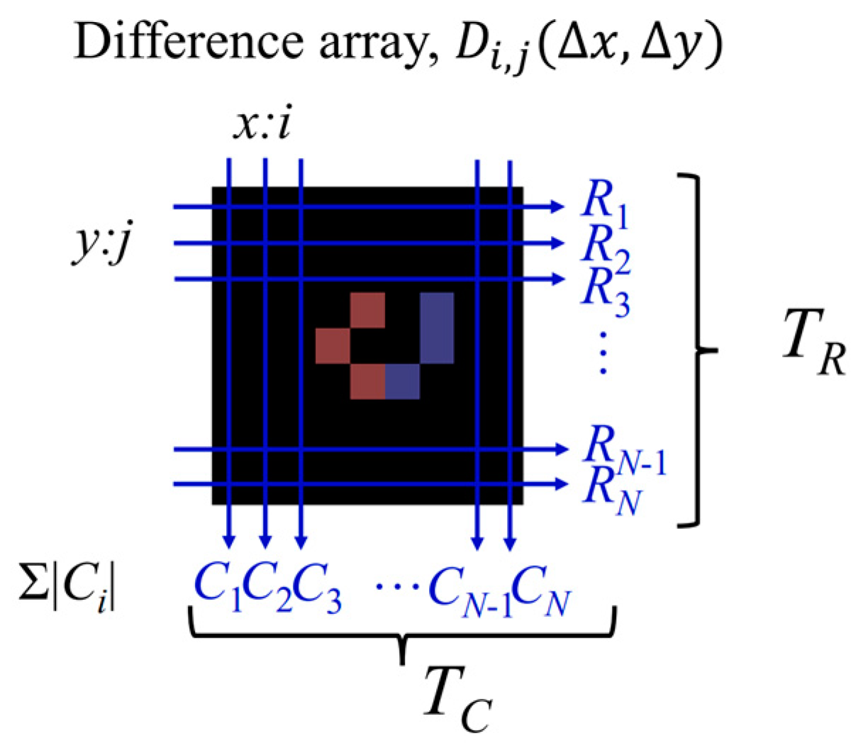
2.2. Discrete Model 2D Motion

This section follows the derivation for the continuous case closely. The difference is that we assume our image, $I_{i,j}$, is discrete. Following Equation (1), over the sampled region $1\le \left(x: i, y: j\right)\le N$,

$$I_{i,j}(∆x,∆y)\approx I_{i,j}\left(\mathrm{0,0}\right)+I_{i,j;∆x}\left(\mathrm{0,0}\right)∆x+I_{i,j;∆y}\left(\mathrm{0,0}\right)∆y,$$

(10)

where $I_{i,j;∆x}\left(\mathrm{0,0}\right)$ and $I_{i,j;∆y}\left(\mathrm{0,0}\right)$ are the partial derivatives of $I_{i,j}\left(\mathrm{0,0}\right)$ with respect to x and y,

$$I_{i,j;∆x}\left(\mathrm{0,0}\right)\approx {[I}_{i,j}(∆x,∆y=0)-I_{i,j}\left(\mathrm{0,0}\right)]/∆x,$$

(11a)

$$I_{i,j;∆y}\left(\mathrm{0,0}\right)\approx {[I}_{i,j}(∆x=0,∆y)-I_{i,j}\left(\mathrm{0,0}\right)]/∆y$$

(11b)

The discrete difference function $D_{i,j}\left(∆x,∆y\right)$ is as follows.

$$D_{i,j}(∆x,∆y)=I_{i,j}\left(∆x,∆y\right)-I_{i,j}\left(\mathrm{0,0}\right)\approx I_{i,j;∆x}\left(\mathrm{0,0}\right)∆x+I_{i,j;∆y}\left(\mathrm{0,0}\right)∆y$$

(12)

We use $D_{i,j}\left(∆x,∆y\right)$ to generate two 1D vectors. The first is the sum of the values in the jth row, yielding $R_j$($∆x,∆y$), a $1\times N$ vector. The second is the sum of the values in the ith column, yielding $C_i\left(∆x,∆y\right)$, an $N\times 1$ vector. Explicitly,

$$C_i\left(∆x,∆y\right)=\sum _{j=1}^N{D}_{i,j}\left(∆x,∆y\right),\hspace{1em}\hspace{1em}\hspace{1em}{R}_j\left(∆x,∆y\right)=\sum _{i=1}^N{D}_{i,j}\left(∆x,∆y\right).$$

(13)

Hence,

$$T_C\left(∆x,∆y\right)={\sum }_i\left|C_i\left(∆x,∆y\right)\right|,\hspace{1em}\hspace{1em}\hspace{1em}{T}_R\left(∆x,∆y\right)={\sum }_j\left|R_j\left(∆x,∆y\right)\right|.$$

(14)

Equations (13) and (14) are illustrated in Figure 1.

For the 1D case, $∆y=0$ or $∆x=0$, in the x and y directions, respectively. We define the following:

$$T_C\left(∆x,∆y=0\right)=\sum _i\left|C_i\left(∆x,∆y=0\right)\right|, T_R\left(∆x,∆y=0\right)=\sum _j\left|R_j\left(∆x,∆y=0\right)\right|,$$

(15)

$$T_C\left(∆x=0,∆y\right)=\sum _i\left|C_i\left(∆x=0,∆y\right)\right|, T_R\left(∆x=0,∆y\right)=\sum _j\left|R_j\left(∆x=0,∆y\right)\right|.$$

(16)

As before, both $T_C\left(∆x,∆y=0\right)$ and $T_R\left(∆x,∆y=0\right)$ are linear functions of $\left|∆x\right|.$ Hence,

$$T_C\left(∆x,∆y=0\right)=P_{C,1}\left|∆x\right|, \mathrm{a}\mathrm{n}\mathrm{d} T_R\left(∆x,∆y=0\right)=P_{R,1}\left|∆x\right|.$$

(17)

Further, if $T_R\left(∆x=0,∆y\right)$ and $T_C\left(∆x=0,∆y\right)$ are linear functions of $\left|∆y\right|$,

$$T_R\left(∆x=0,∆y\right)=M_{R,1}\left|∆y\right|, \mathrm{a}\mathrm{n}\mathrm{d} T_C\left(∆x=0,∆y\right)=M_{C,1}\left|∆y\right|.$$

(18)

From Equations (17) and (18), the linear coefficients $P_{C,1}$, $P_{R,1}$, $M_{C,1}$ and $M_{R,1}$ can be found.

Given these coefficients (M and P), and the values for T_C and T_R for any general motion in 2D, involving any combination of $∆x \mathrm{a}\mathrm{n}\mathrm{d} ∆y$, can we determine the values of $∆x \mathrm{a}\mathrm{n}\mathrm{d} ∆y$ and could we even possibly find the direction of motion?

To examine this situation, we return to the 2D case, i.e., when $∆x\ne 0,\mathrm{a}\mathrm{n}\mathrm{d} ∆y\ne 0,{T_C\left(∆x,∆y\right) \mathrm{a}\mathrm{n}\mathrm{d} T}_R\left(∆x,∆y\right)$ as defined in Equation (14) can be rewritten from Equation (19) as,

$${\mathrm{L}\mathrm{o}\mathrm{w}(T}_C)=\left|P_{C,1}\left|∆x\right|-M_{C,1}\left|∆y\right|\right|\le T_C\left(∆x,∆y\right)\le P_{C,1}\left|∆x\right|+M_{C,1}\left|∆y\right|=\mathrm{U}\mathrm{p}\left(T_C\right),$$

(19)

$$\mathrm{Low}\left(T_R\right)=\left|P_{R,1}\left|∆x\right|-M_{R,1}\left|∆y\right|\right|\le T_R\left(∆x,∆y\right)\le P_{R,1}\left|∆x\right|+M_{R,1}\left|∆y\right|=\mathrm{U}\mathrm{p}\left(T_R\right).$$

(20)

In these equations, we have introduced the upper and lower limiting values of T_C and T_R, i.e., Up(T₋) and Low(T₋), which are defined assuming the validity of our linear approximation, i.e., $∆x$ and $∆y$ are small and Equation (10) is valid. If T_C and T_R could both be described as linear combinations of $∆x$ and $∆y,$ there would be two simultaneous equations for two unknown values. In such a case, $∆x \mathrm{a}\mathrm{n}\mathrm{d}∆y,$ could be unambiguously determined for any 2D motion. However, Equations (19) and (20) emphasize the ambiguity introduced by the use of the absolute value operation and the loss of directional information.

3. Two-Dimensional Simulation Results

In our simulation, we wish to examine the performance of SM for 2D motion estimation, especially the relationship between 2D motion and the corresponding 1D components. To do so, we first present a set of simulations using the standard USAF chart image. In the next section, Section 4, a corresponding set of experimental results illustrating the calibration process is presented.

To start, we define the quadrants, as shown in Figure 2. Any motion in the first quadrant (Q1) can be described as involving components of motion to the right (+x) and up (+y). Similarly, the second quadrant (Q2) involves motion to the right (+x) and down (−y), the third quadrant (Q3) motion to the left (−x) and down (−y), and the fourth quadrant (Q4) to the left (−x) and up (+y). Reference to diagonal motion in Q1, Q2, Q3 and Q4 involves motion along lines at 45°, −45°, −135° and 135°, with respect to the positive x axis.

Recall that SM is based on the calculation of the absolute sum of accumulated grey level changes, T_C and T_R values, and the direction information has been eliminated. To avoid repetition, we only present the simulation and experimental results for Q1. The corresponding results for Q2–Q4 can be found in [22].

In all the simulations presented below, an 8-bit grey level, 780 × 780-pixel USAF chart is first numerically converted to a 16-bit image, using the ‘im2uint16’ Matlab 2018a command. This is then used as the input, or original image, I; see Figure 3a. Next, we visualized this image positioned behind a fixed window, which represents the limiting field of view of the camera. This results in the 760 × 760-pixel windowed images, I_W, shown in Figure 3b, which are then zero-padded up to 1024 × 1024 pixels, I_PW, shown in Figure 3c. For model displacement, the original image, I, is shifted by δ_x behind the window to form the translated image, I_δx.

In order to simulate subpixel motion, bicubic interpolation is applied to the original image before translation. Simpler interpolation methods, e.g., linear and nearest neighbor, have been examined. In general, the Bicubic command which is the default setting for image interpolation in Matlab provides an accurate representation but requires similar computational time to that of the Linear or Nearest interpolation commands. We note that in all simulation results presented here, double precision calculations are used and, in some cases, this was necessary in order to avoid numerical inaccuracy. For each translation step, the same process is followed, i.e., windowing, padding, etc.

Using this input image, we now examine SM. All calculations are performed using an Intel(R) Core (TM) i7-6700 [email protected] GHz with an installed RAM of 32.0 GB.

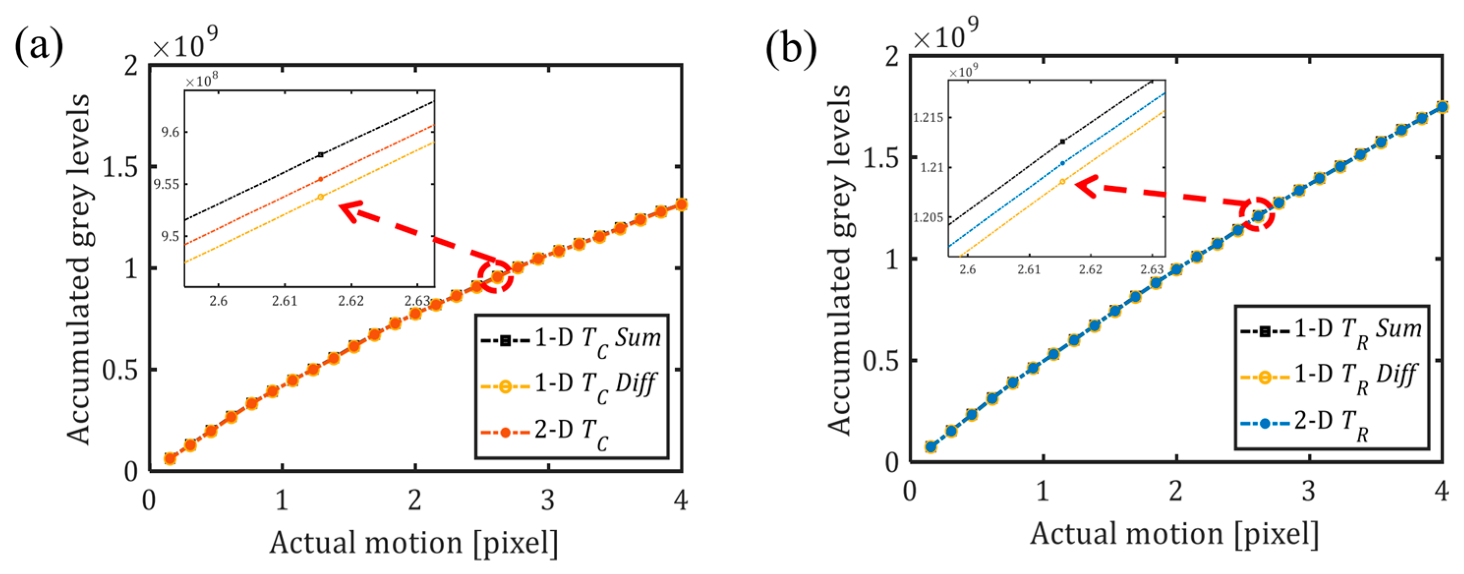
3.1. Subtraction Method: Object without Noise

SM is now applied to examine the same 1D and 2D motion cases. For 1D motion in the +x{+y} direction, the displacement, δx, varies from 1/6.5 to 4 pixels in 26 steps. Two-dimensional motion occurs simultaneously in Q1, in both the x and y directions along the diagonal, y = x, at 45° to the positive x axis. Each step along the diagonal is made up of equal steps in x and y; therefore, both +x and +y vary from 1/6.5 to 4 pixels in 26 steps. The accumulated grey level values (T_C and T_R), i.e., Equation (14), as functions of the translated pixel displacements are presented in Figure 4a,b, respectively. In Figure 4c, the T_R and T_C results shown in Figure 4a,b, and their linear fits are presented. The results for 2D diagonal motion in Q1 are shown in Figure 4d.

We note that the result in Figure 4a corresponds to the case described by Equation (17). The slopes of the line fits to the accumulated grey levels, i.e., the T_C values, over the two regions: (i) 0.15–1 pixels, and (ii) 1–4 pixels, are listed in

Table 1. Piecewise linear fits to simulated data: g = m$\delta$ +c, for motion in Q1. The larger coefficient values are shown in bold text. The quality of the linear fits is indicated by the R² value. Note that this tabulated 1D motion information is used below, in this section, to calibrate the 2D motion.

Q1		+x (m: PC,1 or PR,1)		+y (m: MC,1 or MR,1)		y = x 2D
Range (Pixels)		(i) 0.15~1	(ii) 1~4	(i) 0.15~1	(ii) 1~4	(i) 0.15~1	(ii) 1~4
TC	m c R2	4.328 × 108 −2.67 × 106 0.9994	2.934 × 108 1.697 × 108 0.9946	3.359 × 105 2575 0.9996	2.639 × 105 8.961 × 104 0.9963	4.328 × 108 −2.671 × 106 0.9994	2.934 × 108 1.697 × 108 0.9946
TR	m c R2	2.85 × 105 −632.8 0.9997	2.122 × 105 9.971 × 105 0.9947	5.053 × 108 −6.998 × 105 0.9996	4.168 × 108 1.059 × 108 0.9989	5.053 × 108 −7.044 × 105 0.9996	4.167 × 108 1.059 × 108 0.9989

. In the table, for 1D motion along +x, we list the slopes of the linear fits m, for T_C and T_R, which correspond to the $P_{C,1}$ and $P_{R,1}$ coefficients, respectively. Similarly, for motion along +y, the slopes for T_C and T_R are listed as $M_{C,1}$ and $M_{R,1}$; see Equation (18). The larger coefficient values are shown in bold text. The quality of the linear fits is indicated by the R² value. Note that this tabulated 1D motion information is used below, in this section, to calibrate the 2D motion.

From the table, we note that $P_{C,1}$ >> $P_{R,1}>0$. Similarly, based on the 1D results in Figure 4b, from Table 1, we see that $M_{R,1}$ >> $M_{C,1}>0$. Good quality fits to the 2D y = x results in Figure 4c are shown. To do so quantitively, the values at particular points in Figure 4a,b and their ratios, will be used. For example, from these figures, we see that $\frac{T_R\left(∆x=0,∆y=4\right)}{T_C\left(∆x=4,∆y=0\right)}$ = (1.748 × 10⁹/1.312×10⁹) = 1.33. Furthermore, $\frac{T_R\left(4,0\right)}{T_C\left(4,0\right)}$ = (9.239 × 10⁵/1.312 × 10⁹) = 7.042 × 10⁻⁴; similarly, $\frac{T_C\left(0,4\right)}{T_R\left(0,4\right)}$= (1.119 × 10⁶/1.748×10⁹) = 6.40 × 10⁻⁴. As can be seen, the T_R term in Figure 4a and the T_C term in Figure 4b are very small. The 2D $T_C$ and $T_R$ terms in Figure 4c are almost identical to the corresponding 1D terms in Figure 4a,b.

Based on the results for Q1 presented in Figure 4, we now examine the predictions in Section 2.2 regarding (a) the existence of a linear relationship between the accumulated grey level values and translated distance; (b) the possibility of the expressing 2D motion in terms the corresponding 1D motions; and (c) the existence of upper and lower limits on the values of the 2D accumulated grey level values.

In relation to (a), from Table 1, we see that good quality linear fits exist for all the simulation results, i.e., R² $\approx 1$.

In relation to (b), we examine the results listed in Table 1. It can be seen that the 1D T_C results for +x closely agree with the 2D y = x results. Similarly, the 1D T_R results for +y closely agree with the 2D y = x results. This supports the prediction that the 2D motion can be expressed in terms of the 1D motion.

In relation to (c), let us return to the discussion in Section 2.2 regarding inequalities and limiting values. To define these limits, the Up(T₋) and Low(T₋) expressions in Equations (19) and (20) were introduced. These place limits on the 2D result using the linear fits to the 1D T_R and T_C values given in Table 1. Alternatively, the limits on the 2D simulation results in Figure 4d can be directly calculated using the 1D simulation results in Figure 4a,b. In this case, linear fits are not used. In Equations (21) and (22), we define the 1D T_ Sum and 1D T_ Diff operations as follows:

$$1\mathrm{D} T_C \mathit{Sum} = T_C\left(∆x,∆y=0\right)+T_C\left(∆x=0,∆y\right),$$

(21a)

$$1\mathrm{D} T_C \mathit{Diff} = T_C\left(∆x,∆y=0\right)-T_C\left(∆x=0,∆y\right),$$

(21b)

$$1\mathrm{D} T_R \mathit{Sum} = T_R\left(∆x,∆y=0\right)+T_R\left(∆x=0,∆y\right),$$

(22a)

$$1\mathrm{D} T_R \mathit{Diff} = {T_R\left(∆x=0,∆y\right)-T}_R\left(∆x,∆y=0\right)$$

(22b)

In Figure 5a, the 2D results for T_C in Figure 4d are shown to lie between the sum of the 1D results for T_C in Figure 4a,b, using Equation (21a), and the difference between these same results, using Equation (21b). Similarly, in Figure 5b, the results for T_R in Figure 4d lie between the sum of the values for T_R in Figure 4a,b and their difference; see Equations (22a) and (22b).

For the simulated results presented in Figure 5, if we compare the corresponding T₋ Sum and Up(T₋) values or T₋ Diff and Low(T₋) values, it found that they closely agree. For example, for a displacement value of 1.077 pixels, i.e., at the interface between the line fits in regions (i) and (ii), Up(T_C) = 4.86 × 10⁸ $\approx$ Low(T_C) = 4.853 × 10⁸ > T_C Sum = 4.466 × 10⁸ $\approx$ T_C Diff = 4.459 × 10⁸.

From Figure 5, it can once again be seen that in this case, i.e., when y = x, the SM simulations predict that $T_C\left(∆x,∆y\right)\cong$ $T_C\left(∆x,∆y=0\right)$ and $T_R\left(∆x,∆y\right)\cong$ $T_R\left(∆x=0,∆y\right)$.

Therefore, based on the predictions when y = x shown in Figure 5, we next estimate the general 2D motion case in terms of the corresponding 1D calibration; see Table 1. The 2D motion in Q1 along the trajectories (1) y = 2x, (2) y = x and (3) y = x/2 are examined, and the corresponding accumulated grey levels for these three cases are calculated using SM. The 2D motion estimation results are shown in Figure 6a.

To generate Figure 6a, the 1D piecewise calibration process (see Figure 4 and Table 1) is used to estimate the corresponding 2D motion. To examine 2D motion estimation accurately, a separate 1D calibration process is performed for the 2D motion of y = 2x and y = x/2, respectively. In other words, the corresponding 1D +x from 0 to 2 pixels and 1D +y from 0 to 4 pixels is calibrated for the 2D motion along the y = 2x estimation. Similarly, the 1D +x from 0 to 4 pixels and 1D +y from 0 to 2 pixels is calibrated for 2D motion along the y = x/2 estimation. The chosen lines are arbitrary and illustrative; we have also examined additional angles including some with irrational multipliers with equivalent results but excluded them for brevity.

Using 1D calibration, given the linear coefficients m and c, and the values for T_C and T_R, the linear fits coefficient values for 2D estimation along the trajectories (1) y = 2x, (2) y = x and (3) y = x/2 are listed in

Table 2. The linear fit coefficients for 2D motion examination along the trajectories: y = 2x, y = x and y = x/2.

Data (TC & TR)	y = 2x		y = x	y = x/2
1D Calibration	x: 0~2 y: 0~4	x: 0~4 y: 0~4	x: 0~4 y: 0~4	x: 0~4 y: 0~2	x: 0~4 y: 0~4
m	1.998	2.004	0.9991	0.5036	0.4978
c	0.0018	0.0205	0.0017	−0.0118	−0.0019
R2	0.9988	0.9931	0.9996	0.998	0.9965
RMSE	0.0405	0.0955	0.0237	0.0256	0.0338

. The root mean square error is defined as $RMSE=\sqrt{{\sum }_{i=1}^N{(\mathrm{E}\mathrm{s}\mathrm{t}\mathrm{i}\mathrm{m}\mathrm{a}\mathrm{t}\mathrm{e}\mathrm{d} \mathrm{m}\mathrm{o}\mathrm{t}\mathrm{i}\mathrm{o}\mathrm{n}-\mathrm{L}\mathrm{i}\mathrm{n}\mathrm{e} \mathrm{F}\mathrm{i}\mathrm{t}\mathrm{s})}^2/N},$ where N is the number of translation steps. Once again, the 2D motion can be determined. We note that the simulated results in Table 2 indicate that when the ranges over which the 1D calibrations take place are identical to the range of the 2D motion, the RMSE values are reduced. Furthermore, increasing the range of motion over which the 1D calibration takes place increases the fit (lowers the RMSE).

To explore the accuracy of SM in determining the displacements of the USAF image in Figure 3, a series of 500 displaced images were numerically generated along y = x, from 0 to 10 pixels, i.e., in steps of 0.02 pixels in x and y. For motion along y = 2x, the image is translated by a maximum of 5 pixels in x (250 steps of 0.02 pixels each) and 10 pixels in y (250 steps of 0.04 pixels each). Similarly, along y = x/2, there is a maximum of 10 pixels translated in x (250 steps, 0.04 pixels each) and 5 pixels translated in y (250 steps, 0.02 pixels each). The T_R and T_C accumulated values are calculated using SM from the sequenced 2D displaced images. The 2D motion is estimated by applying the 1D calibration, as shown in Figure 4a,b and Table 1.

The error (in pixels) between the estimated and actual motion is calculated as follows: Error = Estimated motion—Actual motion. The resulting errors in x and y motion for up to a 10-pixel displacement along y = x are shown in Figure 6b,d. The smaller inserted figure shows the same errors over 0–4 pixels.

Piecewise 1D calibration was performed for motions over the ranges of 0–1 for the subpixel region and 1–4 pixels for the super-pixel region. As can be seen in Figure 6b,d, the extremum errors identified over this range are relatively small, i.e., −0.15 (at 1 pixel) and 0.07 pixels (at 2.76 pixels) in x, and −0.06 (at 1 pixel) and 0.038 pixels (at 2.64 pixels) in y. For motion larger than 4 pixels, the error rapidly increased, i.e., −2.75 pixels at 10 pixels, ~27.5% error, due the use of super-pixel calibration, i.e., 1–4 pixels, rather than 1–10 pixels.

A significant error (and discontinuity) appears at one pixel motion. We know that this is a numerical artifact caused by our choice of a piecewise linear fitting during calibration, i.e., use of the sub- and super-pixel displacement regions, as shown in Figure 4a,b. The error is a function of displacement, i.e., it is not a random process, but systematic. This could be avoided by employing a quadratic, cubic or higher-order polynomial fit to the T_R and T_C accumulated values. However, we have intentionally emphasized the linearity of SM, and piecewise linear fitting is simple and effective.

The mean absolute error, MAE = mean(abs(Estimated motion—Actual motion)), was calculated. Small values, e.g., 0.005 pixels in x and 0.004 in y, are indicated in the subpixel region in the small, inserted figures in Figure 6b,d. In the range of 1–4 pixels, the MAE are 0.056 and 0.024 in x and y, and 0.948 and 0.588 in the range of 1–10 pixels in x and y. The error increases significantly over 4 pixels, which again shows that calibration is necessary in the use of SM.

Large and small inserted histograms corresponding to the results presented in Figure 6b,d are shown in Figure 6c,e, respectively. The intervals in the two histograms are 0.2 pixels and 0.01 pixels for motion over the 0–10 pixel and 0–4 pixel ranges, respectively. Examining the two smaller inserted histograms indicates the presence of two clusters of error values. The lower error value cluster predominantly arises in the subpixel range, while the higher error value cluster is dominated by the errors arising in the super-pixel range. This characteristic, which reflects the piecewise linear calibration process, also appears in our experimental results in Section 4.

At the start of Section 3, we noted that bicubic interpolation was used to model the translation of the image by subpixel resolution steps. One question that arises is as follows: what are the effects of the type of interpolation used? For the example presented (y = x and the range of 0–4 pixels), the maximum absolute error difference between results predicted using bilinear and bicubic interpolation were calculated. Maximum values of 0.062 pixels in x and 0.039 in y were found, and we note that the bicubic results were smoother. To avoid numerical artifacts, clearly the choice of interpolation algorithm is important.

The results presented here are explored experimentally in Section 4.3.

3.2. Subtraction Method: Simulated Object with Noise

The object we used for simulation is a binary USAF chart. To examine the robustness of SM, we add random noise into the USAF chart. The random noise is defined by the standard deviation (σ) and the mean value (µ). In the case of SM, the mean value has been subtracted; therefore, we choose the noise with a mean value equal to zero, i.e., µ = 0. The signal to noise ratio (S/N) is calculated by the total power of the signal and noise. As the standard deviation increases linearly, the S/N decreases exponentially. Here, we examine the cases when S/N = 10 (σ = 6619) and S/N = 1 (σ = 6.632 × 10⁴). For the 2D motion along y = x, the results of SM for these two cases, S/N = 10 and S/N = 1, are shown in Figure 7a,b, respectively.

As can be seen in Figure 7, for S/N = 10 and S/N = 1, the SM results show a good linear performance in both the sub- and super-pixel regions. Therefore, it demonstrates that SM is very robust. The experiments using the USAF with a diffuser will be examined in Section 4.4.

4. Two-Dimensional Experiment Results

We now describe our measurement system.

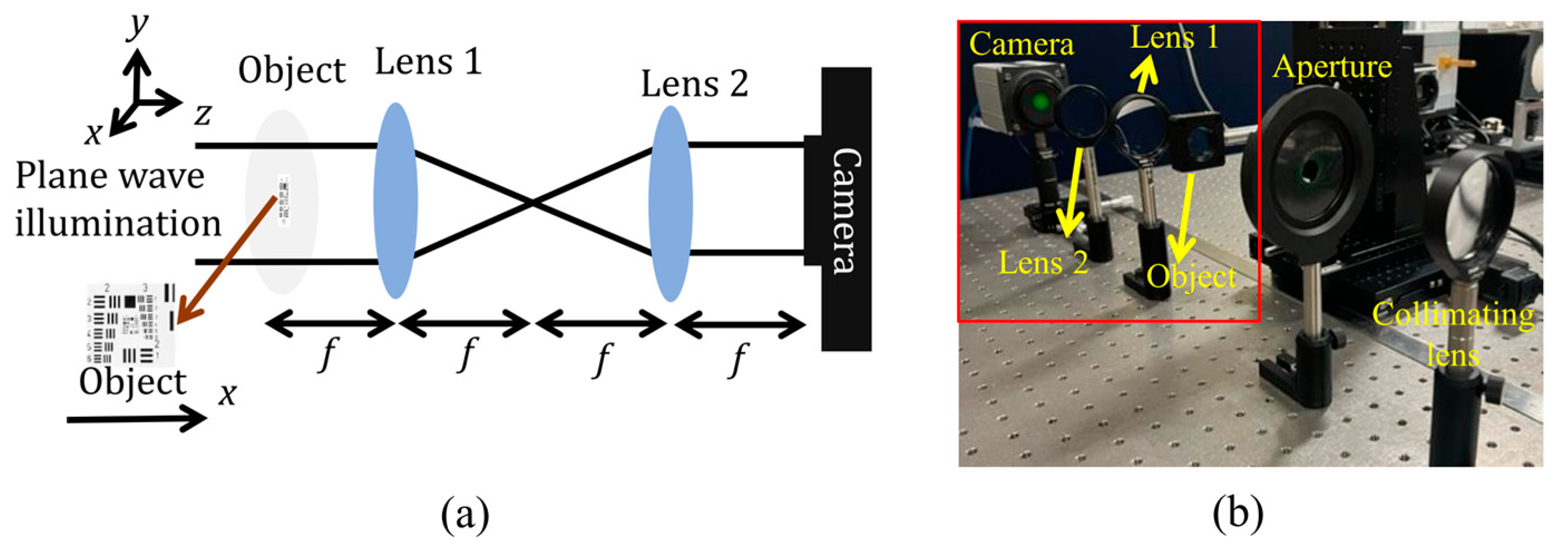
4.1. Image Capturing

To examine the practical performance of our algorithm in determining 2D translations, images were captured using the transmission type 4-f imaging system with unit magnification, shown in Figure 8. The experiments are performed using a 1951 USAF chart. This is illuminated by a collimated plane wave from a diode pumped crystal laser of wavelength 532 nm. A Zyla 5.5 sCMOS camera with 2560 × 2160 pixels and 6.5 µm pixel pitch is used to capture the resulting 16-bit digital images. The object position is altered using a 3D-translation stage, controlled using LabVIEW.

In this section, 1D and 2D motion are examined in detail. In the case of Q1, we begin by capturing a sequence of 14 images in the +x direction {1}, as shown in Figure 9. The motors in the motion stage are then reversed to move the object back to the starting point (0,0). Next, 14 images are captured with the same displacements in the +y direction {2} and once again we return to (0,0). Finally, combining steps in x and y, 14 images are captured along the diagonal direction, corresponding to trajectory {3} as shown in Figure 9.

Each of the adjacent images in the sequences, i.e., along the x and y axis, involve the object being translated by 2 µm (0.3077 pixels). Therefore, the first image, I₀, and the Mth image, I_(M−1)δx, have a relative displacement of (M−1)δx between them. Given M = 14, and δx = 2 µm, then (M−1) δx = 26 µm (~4 pixels), which is the total distance of travel along each axis. In the case of diagonal motion between each image captured, equal steps are performed in x and y. We note that the sample used is a transparent object and the reflection feedback is strong; therefore, during the experiment, the sample has been slightly rotated. This leads to the misalignment between the object and camera plane which can introduce error in the results. As noted, the camera has a total of 2560 × 2160 pixels. In our 1:1 imaging system, the USAF chart only fills a central part of this field of view, 620 × 620 pixels. A selected central region of the image captured by the camera, corresponding to 800 × 800 pixels, is used in our calculations following appropriate zero-padding.

If the illumination intensity varies significantly between image captures, temporal normalization may be necessary. To do so, the intensity in each image is normalized with respect to the sum of 100 × 100 pixels values from the top left-hand corner of each image. This is calculated as follows,

$${I^{\prime }}_{\left(M-1\right)\delta x}=\left(\frac{S_0}{S_{\left(M-1\right)}}\right)I_{\left(M-1\right)\delta x},$$

(23)

where $S_0={\sum }_{i,j}{I}_0\left(i,j\right)$, $S_{\left(M-1\right)}={\sum }_{i,j}{I}_{\left(M-1\right)\delta x}\left(i,j\right)$ and $a\le \left(i,j\right)\le b$. As indicated, we choose a = 1, b = 100. The resulting 800 × 800 data values are next zero-padded up to an array of 1024 × 1024 values. This is the form of the optical image data used to produce the results presented below.

Applying SM, two distinct approaches are used to extract subpixel information. Method 1 refers to the ‘M- -1′ method, and Method 2, refers to the ‘M+q- -M’ method; see [8,19].

4.2. Examination of 2D Experimental Results

In Section 3.1, applying SM, the simulated results for motion in Q1 were presented. Before proceeding to describe the calibration of this method, we first wish to provide some validation of the simulation results.

In Figure 10, experimental results, produced using the USAF chart, which correspond to the simulation results presented in Figure 4, are given. We recall that a 16-bit camara is used in our experiments. The line fits to the data, i.e., the $T_C$ and $T_R$ values, over the two regions: (i) 0.3–1 pixels and (ii) 1–4 pixels, are listed in

Table 3. Piecewise linear fits to experimental data: g = m$\delta$ +c, for motion in Q1.

Q1		+x (m: PC,1 or PR,1)		+y (m: MC,1 or MR,1)		y = x 2D
Range (Pixel)		(i) 0.3~1	(ii) 1~4	(i) 0.3~1	(ii) 1~4	(i) 0.3~1	(ii) 1~4
TC	m c R2	1.592 × 108 2.758 × 107 0.9828	1.123 × 108 8.017 × 107 0.9976	−1.51 × 107 3.573 × 107 0.9914	1.533 × 106 3.469 × 107 0.0367	1.462 × 108 3.654 × 107 0.9924	1.143 × 108 7.018 × 107 0.9989
TR	m c R2	2.673 × 107 2.094 × 107 0.9061	5.356 × 106 5.805 × 107 0.3275	1.825 × 108 3.361 × 107 0.9987	1.48 × 108 8.124 × 107 0.9961	1.851 × 108 4.833 × 107 0.9975	1.511 × 108 7.677 × 107 0.9996

.

We note that in Figure 10a, unlike in Figure 4a, the $T_R\left(∆x,∆y=0\right)$ values are relatively larger. Similarly, in Figure 10b, the $T_C\left(∆x=0,∆y\right)$ values are larger than the corresponding simulation results in Figure 4b.

As noted, in Section 3.2, we wish to compare our experimental and simulation results. We previously examined the results in Figure 4a,b. It was shown for example that $\frac{T_R\left(0,4\right)}{T_C\left(4,0\right)}$ = 1.33. Examining Figure 10a,b, we see that in this case $\frac{T_R\left(0,4\right)}{T_C\left(4,0\right)}$ = (6.67 × 10⁸/5.19 × 10⁸) = 1.28. This indicates a reasonably good quantitative agreement between the simulated and experimental results. However, there are clearly significant differences. Thus, for example, from Figure 10a,b, we can also see that $\frac{T_R\left(4,0\right)}{T_C\left(4,0\right)}$ = (6.53 × 10⁷/5.19 × 10⁸) = 0.126; similarly, $\frac{T_C\left(0,4\right)}{T_R\left(0,4\right)}$ = (4.29 × 10⁷/6.67 × 10⁸) = 0.064. The values of these ratios are much larger than those for the corresponding simulated results in Figure 4a,b.

In Figure 11, the experimental results corresponding to the predictions of our simulation in Figure 5 are presented. We note the agreement is not as close as in the simulation; however, the 2D results are consistently bound by the 1D values (Sum above and Diff below).

In Figure 11a, in agreement with Figure 5a, the measured 2D T_C results, which correspond to displacements in Q1 along the y = x line, lie between the 1D T_C Sum and T_C Diff results, i.e., Equation (21). Similarly, in agreement with Figure 5b, the 2D T_R results lie between the 1D T_R Sum and T_R Diff results, shown in Figure 11b. However, a larger gap separates the 1D T₋ Sum and T₋ Diff results in Figure 11 than in Figure 5. This may be due to experimental errors.

In Figure 12, we compare the 2D results from Figure 10c with the corresponding 1D results in Figure 10a,b.

These experimental results confirm the predictions in Section 2.2, that in this case, i.e., when y = x, $T_C\left(∆x,∆y\right)\cong$ $T_C\left(∆x,∆y=0\right)$ and $T_R\left(∆x,∆y\right)\cong$ $T_R\left(∆x=0,∆y\right)$. However, we again note the larger difference between the 1D and 2D cases than that predicted by our simulations in Figure 4.

In this section, it has been shown that qualitative and quantitative agreements exist between the simulation and experimental results. However, the results presented in Figure 11 are different from those presented in Figure 5. As indicated, some of this difference may arise due to experimental errors. Any calibration of the system will require that both systematic and random errors are included.

4.3. Calibration: 1D and 2D

As discussed in Section 2.2, in order to extract accurate 2D motion information we wish to examine the relationship between the 1D calibration results and the corresponding 2D results. In the case of Q1, we previously discussed expressing the variations along {3}: y = x, in terms of the results for {1}: +x and {2}: +y; see Figure 11. Before proceeding, we recall that in that case, both our simulations and our experimental results in Section 4.2 indicate that $T_C\left(∆x,∆y\right)\cong T_C\left(∆x,∆y=0\right),$ and $T_R\left(∆x,∆y\right)\cong T_R\left(∆x=0,∆y\right),$ for some range of displacement, e.g., $0<∆x<4 \mathrm{p}\mathrm{i}\mathrm{x}\mathrm{e}\mathrm{l}\mathrm{s}$, when moving along y = x; see Figure 5 and Figure 12 for simulation and experimental results, respectively. In this case, when y = x, if we find that $T_C\left(∆x,∆y\right)$ we know $∆x$, and therefore, we also know $∆y$. Therefore, we perform estimation of the general 2D motion case using 1D calibration experimental data. The experimental 2D motion in Q1 along the trajectories (1) y = 2x, (2) y = x and (3) y = x/2 are examined; a similar procedure is performed as in Section 3.1. The corresponding accumulated grey levels for (1) y = 2x, (2) y = x and (3) y = x/2 are calculated using SM. The 2D motion estimation results for these three cases are shown in Figure 13a.

As can be seen in Figure 13a, a general 2D motion along (1) y = 2x, (2) y = x and (3) y = x/2 can be estimated using the 1D calibrated data. The corresponding linear fits to the results in Figure 13a are listed in

Table 4. The linear fit coefficients for 2D motion examination along y = 2x, y = x and y = x/2.

Data (TC & TR)	y = 2x	y = x	y = x/2
1D Calibration	+x: 0~4 pixels          +y: 0~4 pixels
m	2.037	0.9375	0.4453
c	−0.1316	−0.05981	0.02585
R2	0.9811	0.9992	0.9903
RMSE	0.1386	0.0332	0.0475

.

We note that no attempt is made here to correct the systematic error occurring in the experimental results presented in Figure 13a. Therefore, the line fit or estimated 2D motion, i.e., along y = x, does not intersect the origin (0,0) and the point (4,4); see the purple line in Figure 13a. This misalignment indicates that the SM suffers from systematic error when estimating 2D motion.

In Figure 13b–e, we examine the errors present following the previous discussion of the simulation results in Figure 6. The errors in the estimated x and y motion with respect to the desired motion from 0–4 pixels along y = x are shown in Figure 13b,d. In Figure 13b, the smallest error value is 0.028 pixels occurring for a desired motion of at 1.077 pixels, corresponding to a 2.9% error. The largest error value is 0.41 pixels for a 2.308-pixel shift (corresponding to a 17.76% error) in x. In Figure 13d, the smallest error is −0.012 for a 1.077-pixel shift (1.11%) and the highest 0.14 pixels at 2.308-pixel shift (6.7% error) in y.

In Figure 13b, the MAE values are 0.160 and 0.321 pixels in x for the sub- and super-pixel regions. In Figure 13d, the corresponding MAE values are 0.064 and 0.081 pixels in y. This indicates the presence of measurement bias. Systematic errors can arise in our desired motion value due to background lighting fluctuations, system drift (due to temperature variations) or if the motor is improperly calibrated, e.g., the desired motion is not equal to the actual motion taking place (the real object displacement). Optoelectronic noise and mechanical vibration can introduce random errors. These issues are not discussed further here.

The corresponding histograms of Figure 13b,c with 0.02-pixel intervals are shown in Figure 13c,e. The presence of two clusters of error values is again shown in these two histograms, which have similar characteristics to the smaller inserted histograms in Figure 6c,e in simulation.

From the table, good linear fits, with high R² values of 0.9811, 0.9992 and 0.9903; slope values, m, close to the ideals (2~2.037, 1~0.9375 and 0.5~0.4453); and magnitudes of c < 1 are found for motion along the three trajectories: (1) y = 2x, (2) y = x and (3) y = x/2, respectively. As in Table 2, the RMSE value is calculated using the estimated motion and line fits.

4.4. Object with Diffuser

Although the experimental data typically include random noise, to further examine the robustness of the SM for a general object, a layer of diffuse material (paper) is inserted just before and attached to the USAF test target. Both are simultaneously moved by the translation stage. The SM results for 2D motion along y = x are shown in Figure 14.

As can be observed in Figure 14, the accumulated grey level values, T_C and T_R, are the linear function of the desired motion in regions (i) and (ii).

5. Discussion

We have examined a subpixel motion estimation method, called the subtraction method, SM, for 2D motion estimation using 1D calibration. A detailed basis for the use of SM in 2D motion estimation is provided. Both continuous and discrete analyses are presented, and the relationships between the 1D calibration results and the corresponding 2D results are indicated. It is demonstrated that, following careful calibration, the in-plane motion in 2D can be determined. The robustness of the SM is also examined using both simulated and experimental results. Simulations for different noise levels, i.e., S/N = 10 and S/N = 1, are presented, and experiments involving a diffuse speckle field are performed. In the experiments, the RMSE values followed the same trend observed for the simulations with the linear fits for the 2D motion, y = x being better (having a lower RMSE) than for the other two, y ≠ x, cases. We note that the results for 1D motion estimation using SM and CM are compared in detail in [8]. The systematic and random errors have been examined. To avoid repetition, the CM results for 2D motion estimation are not shown here but have been presented in [22].

In all cases, the results show the SM results exhibit highly linear variation. It is shown that, given such linear variation, a change from increasing to decreasing accumulated grey level values indicates a change in direction [8]. When measuring in 2D, tracking the direction of motion becomes critically important. It is also worthwhile to note that SM will be unsuitable for use as a standalone method; some calibration process will be necessary.

SM is a fast method to measure in-plane object motion with subpixel accuracy. It can be used as a complement to standard correlation methods and/or in conjunction with a reported extension of SM [20] to determine the direction which permits an improvement in overall performance. SM offers significant computation time savings (3N²+ 2N) in comparison to the corresponding CM calculation (O (N²log₂N). To quantify this, we note that subtracting two N by N images requires N² operations. Adding across the N rows and down the N columns requires N² + N² operations. Adding the absolute values of the elements of the C and R vectors, to calculate the T_C and T_R, requires dropping the sign bit and 2N operations. Therefore, it only requires 3N² + 2N addition operations and no multiplications.

As noted, when performing experimental measurements to calibrate the system, knowing the relative position of the object with respect to the camera is critically important. Any inaccuracy in controlling the position (the object displacement) will degrade the calibration process. Therefore, methods to correct for systematic and random errors during calibration will be further explored [22].

6. Conclusions

In this paper, we proposed an SM method for quantifying 2D displacements with subpixel accuracy. The theoretical analysis has been driven by both discrete and continuous models. Simulation and experimental results are presented and the corresponding error analysis (between the actual motion and estimated) for 2D motion has been given. The results indicate that any general motion in 2D involving combinations of in-plane motions in x and y can be determined using the SM after a 1D calibration.

Since the method does not indicate the direction of motions but a change in direction, some calibration process will be necessary. However, in conjunction with standard correlation methods and/or recently proposed methods [20], SM offers significant computation time-saving advantages.

Potential applications of this method would appear to exist; for example, with only slight modifications the accumulated grey level values T_R and T_C can be used to perform image stitching, subpixel registration, particle tracking and to determine the frequency of vibration.

References

1. Pan, Z.; Geng, D.; Owens, A. Self-Supervised Motion Magnification by Backpropagating Through Optical Flow. Adv. Neural Inf. Process. Syst. 2024, 36, 1–21. [Google Scholar]
2. Konstantinidis, D.; Stathaki, T.; Argyriou, V. Phase amplified correlation for improved sub-pixel motion estimation. IEEE Trans. Image Process. 2019, 28, 3089–3101. [Google Scholar] [CrossRef] [PubMed]
3. Chi, Y.M.; Tran, T.D.; Etienne-Cummings, R. Optical flow approximation of sub-pixel accurate block matching for video coding. In Proceedings of the IEEE International Conference on Acoustics, Speech and Signal Processing-ICASSP’07, Honolulu, HI, USA, 15–20 April 2007; Volume 1, p. I-1017. [Google Scholar]
4. Tico, M.; Alenius, S.; Vehvilainen, M. Method of motion estimation for image stabilization. In Proceedings of the IEEE International Conference on Acoustics Speech and Signal Processing Proceedings, Toulouse, France, 14–19 May 2006; Volume 2, p. II-277-280. [Google Scholar]
5. Ruan, H.; Tan, Z.; Chen, L.; Wan, W.; Cao, J. Efficient sub-pixel convolutional neural network for terahertz image super-resolution. Opt. Lett. 2022, 47, 3115–3118. [Google Scholar] [CrossRef] [PubMed]
6. Feng, Y.; Yang, T.; Niu, Y. Subpixel computer vision detection based on wavelet transform. IEEE Access 2020, 8, 88273–88281. [Google Scholar] [CrossRef]
7. Yoneyama, S. Basic principle of digital image correlation for in-plane displacement and strain measurement. Adv. Compos. Mater. 2016, 25, 105–123. [Google Scholar] [CrossRef]
8. Wan, M.; Healy, J.J.; Sheridan, J.J. Fast subpixel displacement measurement: Part I: 1-D Analysis, simulation, and experiment. Opt. Eng. 2022, 61, 043105. [Google Scholar] [CrossRef]
9. Guizar-Sicairos, M.; Thurman, S.T.; Fienup, J.R. Efficient subpixel image registration algorithms. Opt. Lett. 2008, 33, 156–158. [Google Scholar] [CrossRef] [PubMed]
10. Karybali, I.; Psarakis, E.; Berberidis, K.; Evangelidis, G. An efficient spatial domain technique for subpixel image registration, Sig. Process. Image Commun. 2008, 23, 711–724. [Google Scholar] [CrossRef]
11. Michaelis, D.; Neal, D.R.; Wieneke, B. Peak-locking reduction for particle image velocimetry, Meas. Sci. Technol. 2016, 27, 104005. [Google Scholar]
12. Tong, W. Subpixel image registration with reduced bias. Opt. Lett. 2011, 36, 763–765. [Google Scholar] [CrossRef] [PubMed]
13. Mas, D.; Ferrer, B.; Sheridan, J.T.; Espinosa, J. Resolution limits to object tracking with subpixel accuracy. Opt. Lett. 2012, 37, 4877–4879. [Google Scholar] [CrossRef] [PubMed]
14. Mas, D.; Perez, J.; Ferrer, B.; Espinosa, J. Realistic limits for subpixel movement detection. Appl. Opt. 2016, 55, 4974–4979. [Google Scholar] [CrossRef] [PubMed]
15. Liu, G.; Li, M.; Zhang, W.; Gu, J. Subpixel matching using double-precision gradient-based method for digital image correlation. Sensors 2021, 21, 3140. [Google Scholar] [CrossRef] [PubMed]
16. Wang, K.; Zhang, Y.; Li, Z. Motion estimation of the common carotid artery wall in ultrasound images using an improved sub-pixel block matching method. Optik 2022, 270, 169929. [Google Scholar] [CrossRef]
17. Marinel, C.; Mathon, B.; Losson, O.; Macaire, L. Comparison of Phase-based Sub-Pixel Motion Estimation Methods. In Proceedings of the IEEE International Conference on Image Processing (ICIP), Bordeaux, France, 16–19 October 2022; pp. 561–565. [Google Scholar]
18. Tu, B.; Ren, Q.; Li, Q.; He, W.; He, W. Hyperspectral image classification using a superpixel-pixel-subpixel multilevel network. IEEE Trans. Instrum. Meas. 2023, 72, 5013616. [Google Scholar] [CrossRef]
19. Wan, M.; Healy, J.J.; Sheridan, J.T. Fast, sub-pixel accurate, displacement measurement method: Optical and terahertz systems. Opt. Lett. 2020, 45, 6611–6614. [Google Scholar] [CrossRef] [PubMed]
20. Healy, J.J.; Wan, M.; Sheridan, J.T. Direction-sensitive fast measurement of sub-sampling-period delays. In Proceedings of the 8th International Conference on Signal Processing and Integrated Networks, SPIN-2021, Noida, India, 26–27 August 2021; pp. 228–232. [Google Scholar]
21. Ferrer, B.; Tomás, M.B.; Wan, M.; Sheridan, J.T.; Mas, D. Comparative Analysis of Discrete Subtraction and Cross-Correlation for Subpixel Object Tracking. Appl. Sci. 2023, 13, 8271. [Google Scholar] [CrossRef]
22. Wan, M. Optical Imaging Techniques in the THz Regime. PhD Thesis, University College Dublin, Dublin, Ireland, 2021. [Google Scholar]
Figure 1. Illustration of the calculation for Equations (13) and (14) [19].
Photonics 11 00625 g001
Figure 2. Motion in the four quadrants. In this paper, simulation and experimental results are presented for Q1.
Photonics 11 00625 g002
Figure 3. The windowing and zero-padding processing for image simulation. (a) The original image with 780 × 780 pixels; (b) the central part of (a) having 760 × 760 pixels, IW; (c) zero-padding, IPW, of (b) with 1024 × 1024 pixels.
Photonics 11 00625 g003
Figure 4. The SM results for the USAF chart for motion in Q1; (a) 1D motion in +x, (1D,+x), i.e., giving T C x , y = 0 and T R x , y = 0 ; (b) 1D, +y, i.e., giving T C x = 0 , y and T R x = 0 , y ; (c) 1D motion, T R x , y = 0 , from (a), and T C x = 0 , y , from (b); (d) 2D motion along the path y = x, (2D, y = x), i.e., giving T C x , y and T R x , y . Two regions are separated by green line: (i) subpixel at 0.15–1 pixels, and (ii) super-pixel at 1–4 pixels.
Photonics 11 00625 g004
Figure 5. The 2D results when y = x lies between the sum, TSum, and the difference, TDiff, of the 1D results: (a) TC and (b) TR. This figure clearly indicates that the 2D TC results and the 2D TR results are in this case practically identical (within a fraction of a percentage point) to the corresponding 1D TC and 1D TR results.
Photonics 11 00625 g005
Figure 6. (a) Simulated 2D motion in Q1 along the estimated trajectories (1) y = 2x, (2) y = x and (3) y = x/2. Accumulated grey level values are converted to displacements using 1D calibration (1D, +x and 1D, +y) shown in Table 1. The linear fits to the estimated motion are found; see Table 2. (be) The errors in estimated motion for the y = x case are examined. The errors for (b) the x motion and (d) the corresponding y motion for displacements of 0–10 pixels (inserted figure 0–4 pixels) are presented. (c,e) The corresponding histograms are shown for the results in (b,d).
Photonics 11 00625 g006
Figure 7. SM results for the USAF chart with noise for 2D motion in Q1 along y = x. (a) S/N = 10 and (b) S/N = 1.
Photonics 11 00625 g007
Figure 8. (a) Schematic diagram of the 4-f optical imaging systems, f = 10 cm, M = 1; (b) experimental setup. The red box represents (a).
Photonics 11 00625 g008
Figure 9. Trajectories used in the experiments in Q1.
Photonics 11 00625 g009
Figure 10. Application of SM to experimental data. These results for the USAF chart correspond to the simulated results in Figure 4. Motion in Q1; (a) 1D motion in +x, i.e., giving T C x , y = 0 and T R x , y = 0 ; (b) 1D motion in +y, i.e., giving T C x = 0 , y and T R x = 0 , y ; (c) 2D motion along y = x, i.e., giving T C x , y and T R x , y .
Photonics 11 00625 g010
Figure 11. The 2D experimental results, 2D T, when y = x, lie between the sum, T Sum, and the difference, T Diff, of the 1D results for (a) TC and (b) TR. No corrections for systematic experimental errors are included.
Photonics 11 00625 g011
Figure 12. Comparison between the experimental 2D accumulated grey level results and the corresponding 1D results for (a) T C and (b) T R . No corrections for systematic experimental errors are included. This figure experimentally demonstrates that the 2D TC results and the 2D TR results are practically identical (within a fraction of a percentage point) to the corresponding 1D TC and 1D TR results.
Photonics 11 00625 g012
Figure 13. (a) The experimental 2D motion in Q1 along y = 2x, y = x and y = x/2 estimation using 1D calibration (1D, +x and 1D, +y). The linear fits to the estimated motion are performed; see Table 4. The error for (b) x motion and (d) the corresponding y motion for displacements of 0–4 pixels are presented. (c,e) are the corresponding histograms for the results in (b,d).
Photonics 11 00625 g013
Figure 14. The SM results for the USAF chart with a diffuser for 2D motion in Q1 along y = x.
Photonics 11 00625 g014