Abstract
Tilt-to-length (TTL) coupling noise arises from angular misalignments of interfering beams in optical path length (OPL) measurements and significantly impacts the accuracy of interferometry measurement systems. This paper focuses on geometric TTL coupling in a test mass (TM) interferometer and examines how an imaging system influences TTL noise suppression. First, the analytical expression of the geometric TTL coupling in a TM interferometer with alignment errors is derived and confirmed through numerical simulation. Subsequently, an imaging system is incorporated into the geometric model and the corresponding analytical expressions are obtained under two common conjugate relationships. Nevertheless, the TTL coupling remains beyond the requirement of TM interferometer, as the residual TTL coupled with alignment errors persists even with the imaging system. Therefore, an optimal position of the imaging system capable of eliminating the second-order term of the TTL coupling is determined. Meanwhile, the first-order term can be mitigated through in-orbit calibrations. These findings offer valuable guidance for the design and adjustment of imaging systems in space-borne gravitational wave detection missions, which require high-precision laser interferometry.
1. Introduction
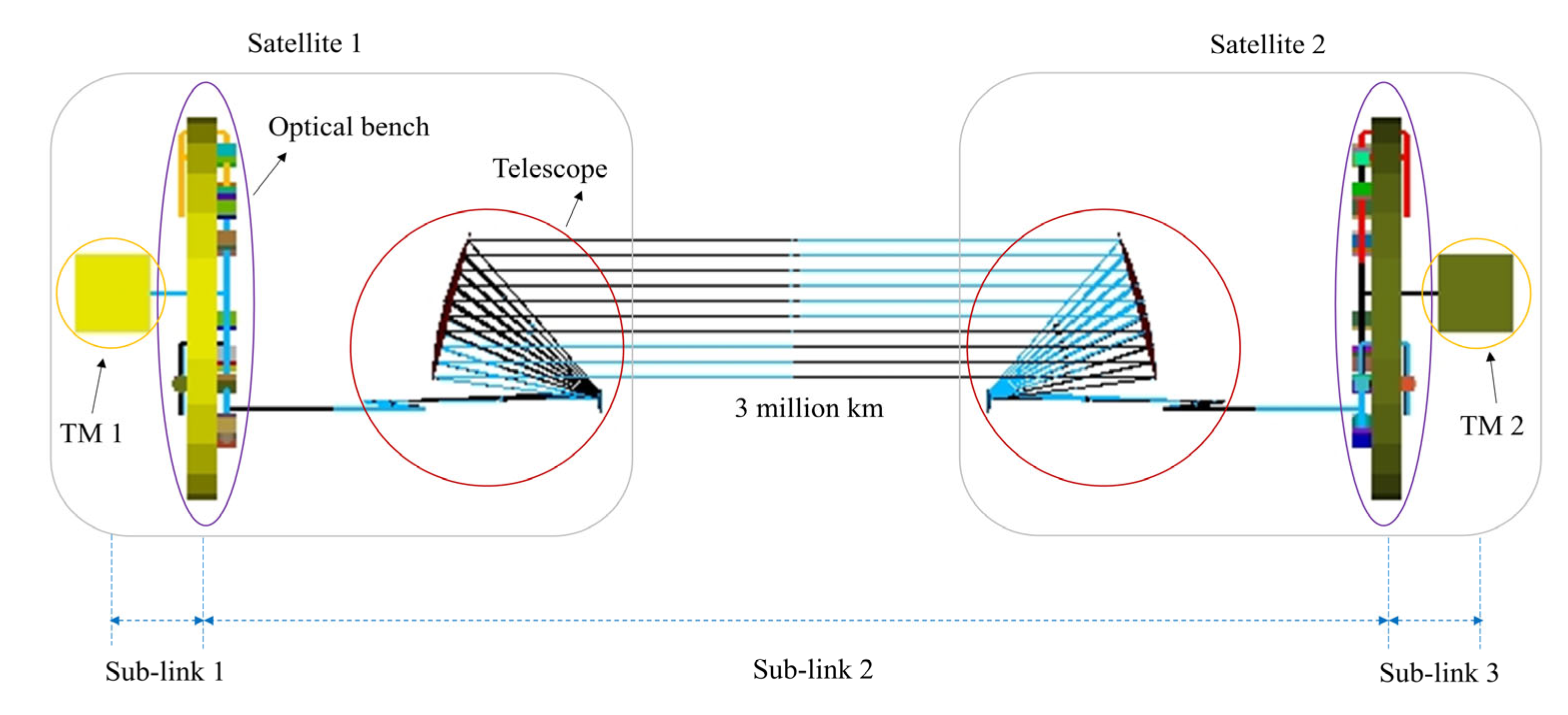
Space-borne and long-baseline laser interferometers such as the Laser Interferometer Space Antenna (LISA) [1,2], the Taiji program [3,4,5,6,7], and the Tianqin program [8,9] aim to detect gravitational waves in the frequency band within 0.1 mHz–1 Hz. In each interferometer, there are three spacecraft forming an equilateral triangle with arm lengths of millions of kilometers, and each satellite has two free-floating test masses (TMs) enclosed by gravitation reference sensors (GRSs), two optical benches inside for guiding the beams to interfere, and two telescopes to send (receive) the expanding laser beam from the local (distant) optical bench to (from) the distant (local) satellite. As illustrated in Figure 1, in order to measure the distance fluctuation between two reference objects (i.e., TMs) for detecting their gravitational waves, the laser link can be split into three sub-links whose length variations are measured via independent interferometers. The distance fluctuation of the TMs relative to the local satellite (sub-link 1 and sub-link 3) is measured by the TM interferometer, and the distance fluctuation between the two satellites (sub-link 2) is measured by the long-arm interferometer [2]. However, the angular jitters of the measurement beam due to the unintended tilt motions of the TM generate the misalignment of the two interfering beams and couple into the optical path length (OPL) readout, which is called tilt-to-length (TTL) coupling noise. Similarly, the unavoidable jitters of the satellite couple into the length readout in the long-arm interferometer, introducing TTL coupling as well. The TTL coupling is a considerable noise source in high precision laser interferometry [10,11,12,13] and is considered to be the second largest contributor to the noise in space-borne gravitational wave detection missions [14]. Therefore, effective approaches to remove or suppress TTL coupling need to be investigated.

Figure 1.
Schematic diagram of a single arm of the Taiji program. The laser link between two TMs consists of three sub-links. The two TM interferometers measure the distance fluctuation between TM 1 and satellite 1 (sub-link 1), TM 2 and satellite 2 (sub-link 3), and the long-arm interferometer measures the distance variation between the two satellites (sub-link 2). The optical bench on each satellite houses several interferometers that utilize identical telescopes for both sending and receiving beams between satellites.
Generally, imaging systems are designed through imaging the center of rotation of the beam onto the detector, causing no beam walk and unchanged OPL despite the jitter of the TM, and the TTL coupling decreases in numerical simulations [15,16]. With regard to TTL coupling experiments, the AEI team made significant efforts to create the four generations of interferometers [15,17]. In the first generation of the large detector heterodyne interferometer, to remove the longitudinal movement of the conventional actuator, which introduces a tilted beam from the measured signal behind the imaging system, a large SEPD (single-element photodiode) only sensing the actuator movement was introduced according to the research that indicated TTL coupling can vanish when two equal Gaussian beams interfere on a very large SEPD [18]. However, the two interfering beams generated by different fiber injections have different beam parameters, arousing additional TTL coupling. To overcome the uncertainty in the beam parameters, a proof-of-principle experiment with one laser source was built in the second generation of the large detector homodyne interferometer [19], and the TTL coupling was mitigated by two orders of magnitude through a two-lens imaging system. However, the homodyne interferometry in this setup is not fully representative for LISA, which performs the experiment featuring unequal beams and heterodyne readout. To solve the problems in the previous first and second TTL coupling experiments, a pinhole sensing only the longitudinal movement of the actuator was made in the third generation of the LISA optical bench testbed, which can mimic the tilted beam from a TM or telescope [12,14,15,20]. Furthermore, a two-lens and four-lens imaging system were designed and tested to prove the suppression of the TTL coupling, both satisfying the LISA requirement that the TTL coupling should be within in the beam tilt angle of [12]. However, the setup in the LISA testbed is complicated and has high requirements for its construction and alignment, and the setup is not suitable for more universal tests of varying interferometric designs and beam parameters for most optical components’ glueing onto the baseplate. To resolve the troublesome difficulty regarding the actuation error and lack of flexibility in the LISA testbed, an actuator without longitudinal movement was implemented in the fourth generation of advanced tilt actuators (ATAs) which provided a tilted beam and simultaneously measured its motion by dedicated interferometers to be subtracted from the length readouts [17]. In a TM scenario, the TM is replaced with the ATA in the original optical layout of the TM interferometer, and the ATA is placed in the intended rotation point to test imaging systems. Although the TTL coupling in the above ground experiments is mitigated below the required level, either a beam rotating around a fixed point (the test bed does not feature a TM) represents the reflection point on the rotating TM, or the position of the imaging system is constantly adjusted to reduce the TTL coupling, which is significantly difficult to operate in orbit for space-borne gravitational wave detection missions.
Another strategy to remove TTL coupling from the readout is data post-processing [21] through a dedicated fit model [10,22], which was successfully applied to the LISA Pathfinder by intentionally tilting the TM and measuring the output. To sufficiently model the underlying mechanisms resulting in the observed TTL coupling, and considering that the subtraction method requires a good signal-to-noise ratio and the range of successful subtraction is limited, an analytical TTL model accounting for all coupling mechanisms present in the LISA Pathfinder was derived [23,24,25,26]. However, an imaging system is not considered in the analytical model, which is utilized to mitigate TTL coupling to a deductible level in space-borne gravitational wave detection missions like LISA or Taiji.
Considering that it is difficult to completely simulate the jitter of an in-orbit TM in a ground experiment, and that the position of the imaging system needs to be determined in the optical bonding process, the analytical expression of the geometric TTL coupling with the imaging system in a TM interferometer is derived in this paper. We find that part of the TTL coupling is eliminated through the introduction of the imaging system, but there is still residual coupling which can be subtracted by in-orbit calibration. Furthermore, the optimal position of the imaging system is deduced, wherein the TTL coupling can be theoretically removed via the placement of the imaging system. This conclusion provides valuable insights and useful guidance for mitigating the TTL coupling in gravitational wave detection programs like LISA or Taiji.
This paper is organized as follows: the theoretical model of the geometric TTL coupling effect in a TM interferometer is given and the accuracy of the corresponding analytical expressions is verified by numerical simulation in Section 2. Then, the imaging system is introduced in the above model and the corresponding TTL analytical expressions under the two typical conjugate relationships are investigated, and also the optimal position of the imaging system is obtained, in Section 3. The TTL theoretical models with the imaging system are confirmed via the numerical simulations, and the sensitivity analysis between the TTL and the optimal position offset is implemented in Section 4. Finally, a summary of the theoretical models and numerical results analysis is given in Section 5.
2. Geometric TTL Coupling Effect in the TM Interferometer
The LISA requirement for TTL coupling is within in the beam tilt angle of . However, for the Taiji program, whose system parameters may be different from LISA, the requirement can also be a little different. Here, taking the TM interferometer of the Taiji program as an example, the TTL coupling noise budget is and the angle jitter of the TM is controlled to ( after division), with the static angle deviation being , i.e., the Taiji requirement for the TTL coupling in TM interferometers is less than @ . Such astringent requirement necessitates an in-depth investigation of TTL coupling, particularly its generation mechanisms.
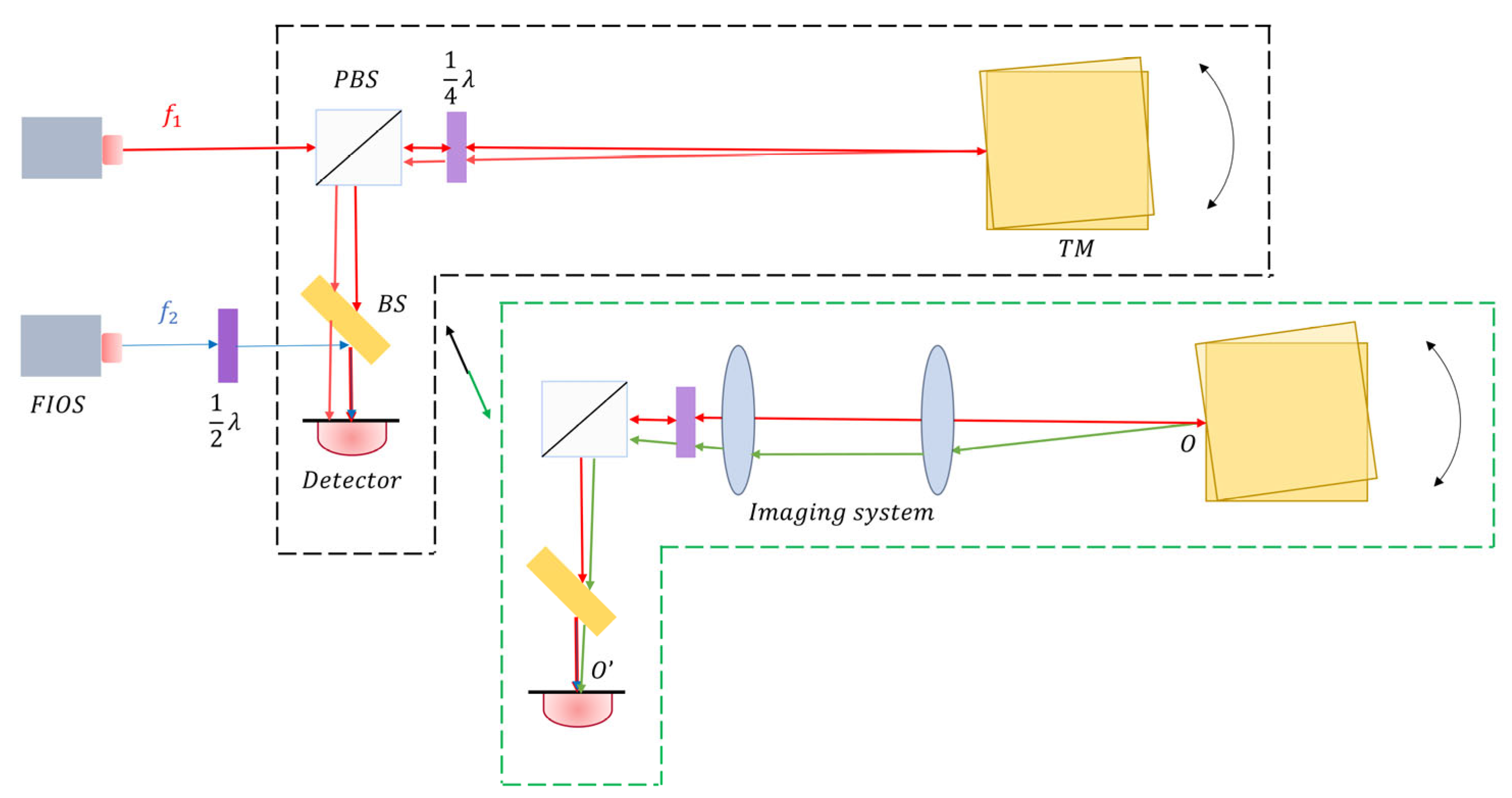
Taking the Taiji program as an example, a sketch of the TTL coupling in the TM interferometer is illustrated in Figure 2. As shown in the black dotted frame of Figure 2, the laser beam is divided into two beams and tuned by two AOMs (Acoustic-Optic Modulators) to generate the reference beam (depicted in blue) and the measurement beam (depicted in red) with the frequency difference of . The measurement beam passes through a PBS (Polarizing Beam Splitter) and (quarter waveplate) in turn, and reaches the hypothetically perfectly aligned TM’s surface. After reflecting off the TM’s surface, it transmits through the again and reflects on the PBS, then interferes with the reference beam transmitting through the at the BS (Beam Splitter) and hitting the center of the detector. However, the measurement beam will deflect away along with the rotation of the TM and the incident position deviates from the center of the detector, as depicted in the black dotted frame of Figure 2, thus introducing the TTL coupling. This specific noise is considered to be the second largest contributor to the noise in space-borne gravitational wave detection [14]. Therefore, a full understanding of the mechanisms of TTL coupling is very significant for TTL reduction and post-processing.

Figure 2.
Schematic diagram of a TM interferometer. In the black dotted frame, the measurement beam (red) is reflected from the tilting TM, while the reference beam (blue) does not change, causing the optical path length difference (OPD) between the two interfering beams. In the green dotted frame, the imaging system is designed to image the point of reflection from the TM () onto the center of the detector (), causing the OPL to remain unchanged, independently of the jitter of the TM (green), based on the Fermat principle. FIOS = Fiber Injector Optical Subassembly, BS = Beam Splitter, TM = test mass, PBS = Polarizing Beam Splitter, = quarter waveplate, = half waveplate.
For a better understanding and clear description of the geometric TTL coupling present in the TM interferometer, we can render the prior image into a more simplified version, isolating the TM and detector, and minimizing the optical path of the fixed reference beam, as depicted in Figure 3. In the geometric TTL coupling model, the measurement beam cannot transmit absolutely vertically to the TM surface due to the alignment error of the detector . Further, there is an initial position deviation of and between the reflection point and the rotation center , which are the longitudinal and lateral deviation, respectively. In addition, denotes the optical path of the reflected beam without the assembly and alignment errors. Before the rotation of the TM, the measurement beam is nominally incident to point on the TM’s surface with the angle of from the point , and hits the point of the detector after reflecting from the TM. When the TM rotates around the point with the angle , the measurement beam is reflected at point and reaches point of the detector; thus, the OPL changes correspondingly. The variation of the OPL is the geometric TTL coupling, which is related to the angle fluctuation . Next, we will analyze the theoretical model to obtain the analytical expression, and implement the simulation computations to validate the result.
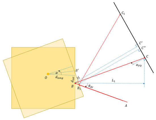
Figure 3.
Schematic diagram of the simplified geometric TTL theoretical model. The OPL changes from the length ( to to ) to the length ( to to ) owing to the rotation of the TM. and denote the initial angular deviation when installing and adjusting the interferometer. and define the longitudinal and lateral displacement between the center of rotation and the point of reflection, respectively. The direction and angle exhibited in the graph are positive, and on the contrary, they are negative.
2.1. Theoretical Model
First of all, it is easy to calculate the length of through the geometric relationships as follows:
thus, the distance between the reflection points before and after the TM’s rotation can be calculated in the following equation:
Then, the vertical distance from to the detector is given as follows:
thus, we can calculate the vertical distance from to the detector:
then, the reflection arm length after the rotation of the TM is calculated as well:
In summary, we can obtain the corresponding OPD before and after the rotation of the TM in the following equation:
In actuality, the jitter of the TM is very small in the space-based gravitational wave detections like LISA or Taiji, and thus the Taylor series to second-order near zero is performed to simplify and improve the analysis of the expression:
By differentiating Equation (), we derive the TTL coupling coefficient , which measures the sensitivity of the OPD to angle fluctuation. Considering that the noise budget of space-borne gravitational wave detections for TLL coupling noise is , along with the jitter amplitudes of the TM under electrostatic control in the range of hundreds of , and accounting for assembly and alignment errors such as , , , and , we exclude contribution factors smaller than . As a result, we obtain the TTL coupling coefficient and the simplified OPD as follows:
Further, is generally very small and can be ignored; thus, the TTL coupling coefficient and the OPD are simplified as follows:
According to Equation (), the transverse component between the center of rotation and the reflection point contributes to the first-order term, and the combination of and the longitudinal component between the center of rotation and the reflection point introduces the second-order term. By substituting the structural parameters and alignment errors of the Taiji program, it can be estimated that the maximum values of the OPD and TTL coupling are in the order of 100 nm and , respectively, which greatly exceed the Taiji and LISA programs’ requirements.
2.2. Numerical Simulation Verification
Building on the theoretical model of the geometric TTL coupling effect outlined in Section 2.1, the numerical simulation of the analytic expression will be verified in this section. Here, the optical model is established and geometric ray tracing is carried out in the ASAP (2010) optical simulation software, then the OPD and TTL coupling are calculated and analyzed using MATLAB (R2018b). The combination of ASAP and MATLAB has been successfully validated in previous studies [27], so it is employed here.
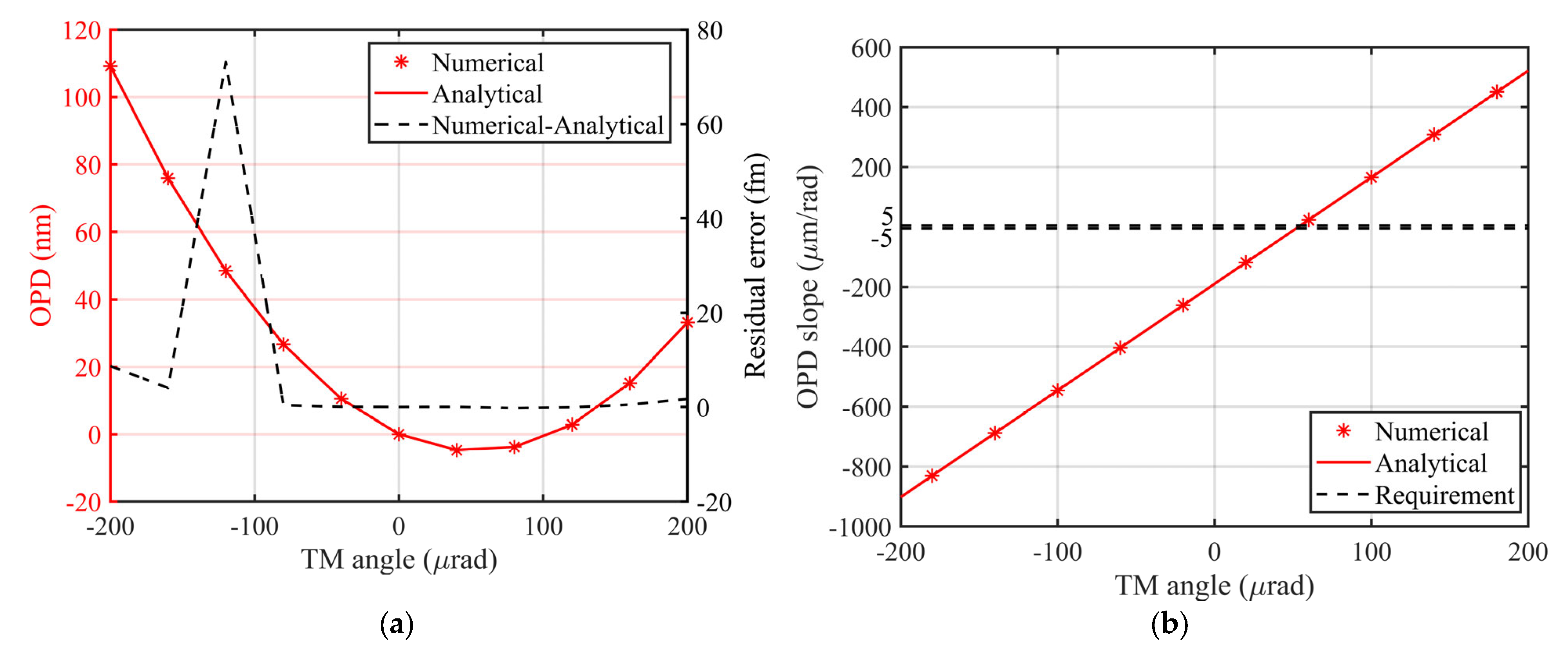
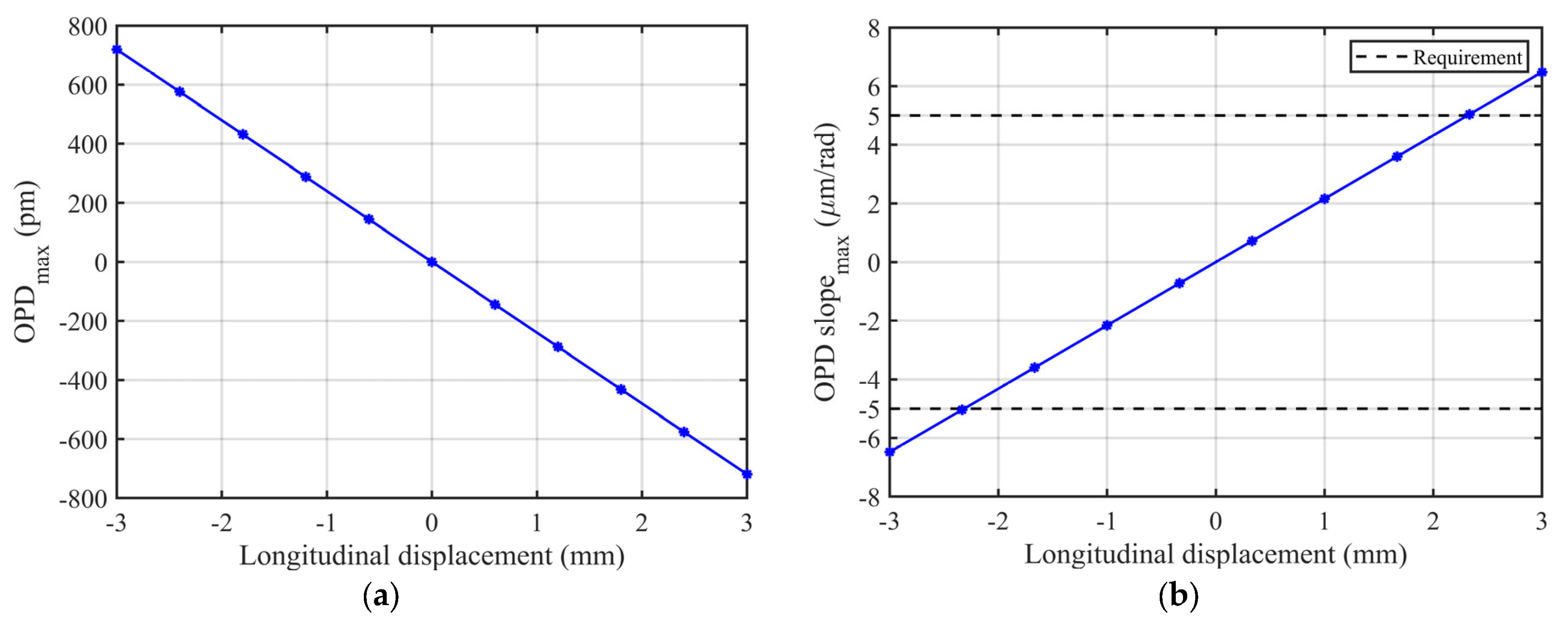
Taking the optical model of the TM interferometer in the Taiji program as an example, the Gaussian optical model in the optical simulation software is set up as follows: , , and . The angular dynamic range of the TM’s rotation is . The corresponding simulation results, illustrated in Figure 4, show that the analytical expressions and simulation outcomes (represented by red solid lines and asterisks, respectively) align closely. The residual error, which arises from the series expansion of the analytical model in Equation (), is less than 0.073 pm. This demonstrates the accuracy of the theoretical model of the geometric TTL coupling effect.
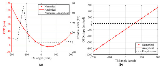
Figure 4.
Numerically and analytically computed OPD (a) and OPD slope (b) of the geometric TTL coupling model of the TM interferometer. The numerical values are marked with red asterisks, while the analytical expressions are solid lines, and the residual error is represented by a black dotted line in the right longitudinal axis.
However, as shown in Figure 4b, the TTL coupling significantly exceeds the Taiji requirement, indicating the need for additional measures, such as an imaging system, to suppress the TTL coupling.
3. Geometric TTL Coupling Effect with Imaging System in the TM Interferometer
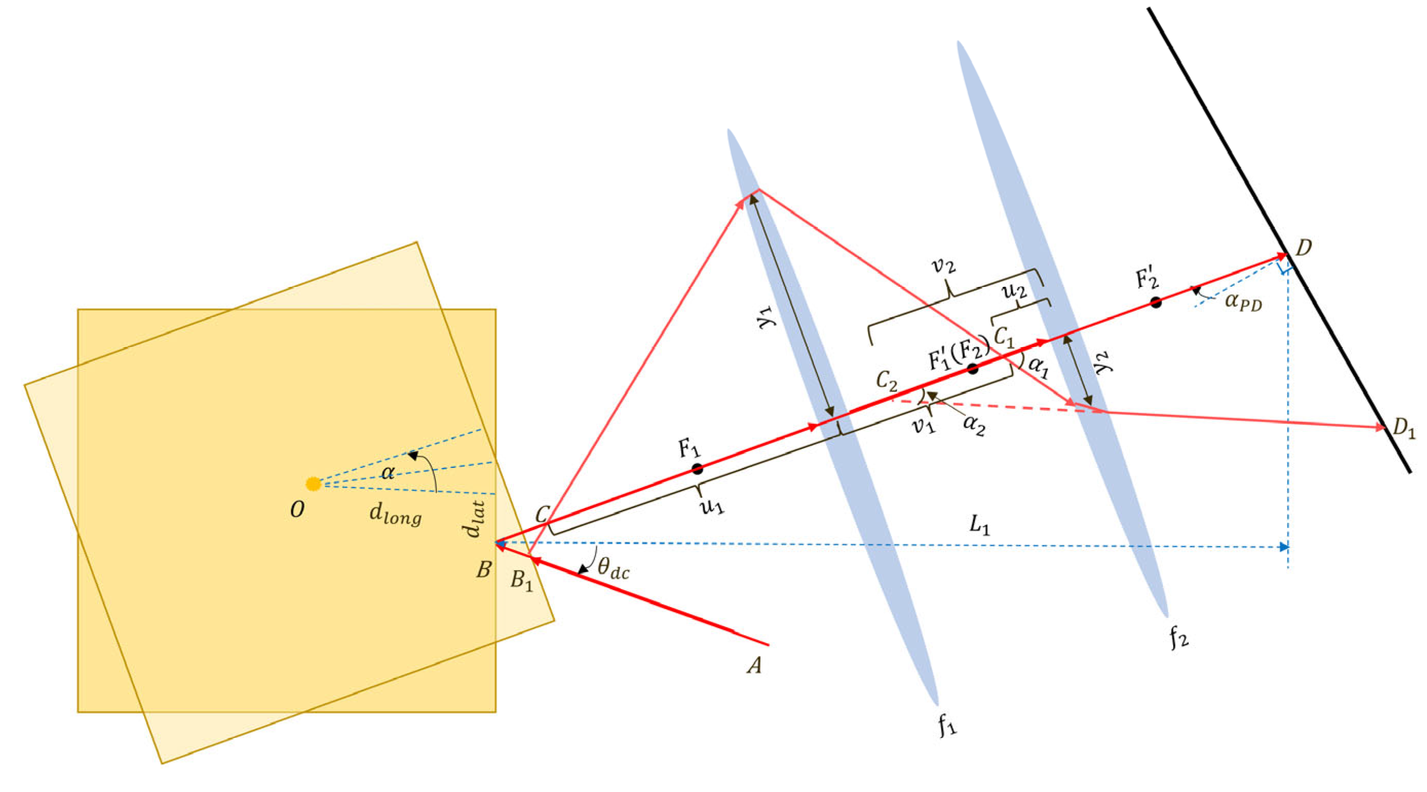
In Section 2.1, we scrutinize the comprehensive theoretical model of TTL coupling within the TM interferometer and provide the associated analytical expression. This scrutiny reveals that the first- and second-order terms originate from lateral and longitudinal deviations between the reflection point and the center of rotation, respectively. To subdue the TTL coupling, an imaging system is employed by projecting the center of rotation of the TM onto the center of the detector, as illustrated within the green dotted frame of Figure 2. For accurate comparison with the geometric model without the imaging system, we also consider the assembly and alignment errors , , , and in the theoretical model, as illustrated in Figure 5. To derive the analytical expression of the complete geometric model following the introduction of the lens group, we first need to focus on the positions of the image point, and , where the intersection between the optical axis and the reflected beam after TM rotation passes through the confocal imaging system and in sequence, as explained below.
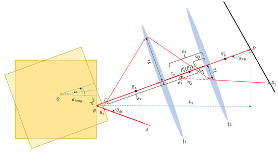
Figure 5.
Schematic diagram of the simplified geometric TTL theoretical model when introducing the imaging system. The OPL changes from the length ( to to to ) to the length ( to to to to to ) owing to the rotation of the TM. and are the object focus of the lens and , respectively, and and are the image focus of the lens and , respectively. and are the image point of passing through the afocal optical system and , respectively. and are the object distance and image distance of imaging through , respectively, and and are the object distance and image distance of imaging through the , respectively. and are the angle between the optical axis and the beam passing through the lens and , respectively. The definitions of , , and are the same as those in Figure 3.
3.1. Theoretical Model
The first part of the reflected OPLs to the point are calculated as follows:
where the and are the OPLs before and after the rotation of the TM, respectively. In order to deduce the OPL of point after passing through the lenses and , we successively calculate the positions of the image points and of point transmitting through the two lenses. First of all, the position of the image point passing through the first lens is obtained according to the imaging theorem [28]:
In the formula above, represents the distance from the point to the center of the first lens , which varies depending on the position of the imaging system. The image distance of the first imaging of the point can be calculated as . Since both lenses in the defocus system share the same focus point, the object distance of the second imaging is determined by . Thus, we can calculate the image distance of the second imaging based on the imaging theorem [28] as follows:
The sign of is negative, i.e., the object point and the image point are on the same side of the lens ; accordingly, the distance is calculated as follows:
In order to trace the OPL from the image point to the detector, we assume that the heights of the beam in the imaging system and are and , respectively. The formular can be easily derived from the geometric relationships, giving us the tangent value of the angle (i.e., the angle between the optical axis and the beam passing through the lens ) after the rotation of the TM:
Similarly, the height of the beam in the lens and the tangent value of the angle (i.e., the angle between the optical axis and the beam passing through the lens ) after the rotation of the TM are calculated, respectively, as follows:
Then, we can obtain the distances and , which represent the distances from the point to the detector before and after the rotation of the TM, respectively:
In summary, in the geometric model with the imaging system, the OPD is calculated by subtracting the OPL after the TM’s rotation from the OPL before the TM’s rotation, which is expressed as follows:
Among them, the , meaning the OPL from the point to the point , can be easily obtained through the geometric relationship in Figure 5:
In the above equation, and denote the extra OPLs introduced in the middle of the lenses and due to the refractive index difference between the lenses and the air, respectively. As the object point and the image point are conjugate, according to the Fermat’s theorem, we can find out the meaning the OPL from the point to the point is as follows:
After substituting Equations () and () into (), we calculate the OPD in the geometric model of the TTL coupling after introducing the imaging system in the following:
For describing the position of the imaging system more clearly, we define the distance from the reflection point to the first lens as in the following:
By substituting the above equation into Equation () and implementing the Taylor series to second-order around zero, we can obtain the replaced by :
Similarly, the contribution items which are much smaller than are omitted, and thus the TTL coupling coefficient is obtained:
In order to express the above expression more clearly, we define , the above equation is changed to the following:
Further, is generally very small and can be ignored; thus, the TTL coupling coefficient and the OPD are simplified as follows:
Meanwhile, the simplified expression between the OPD and the angle is obtained in the following equation:
From the above formula, it is evident that contributes to the first-order term. and , which consists of , , , and , contribute to the second-order term of the TTL coupling. In addition, the first-order term can be subtracted through in-orbit calibration and the second-order term can be eliminated by identifying the optimal position for the imaging system, which will be addressed in the following sections.
So far, we have obtained the complete analytical expression of the geometric TTL after the introduction of the imaging system, which is not only related to the assembly and alignment errors, but also to the position of the imaging system. Ideally, the optimal position of the imaging system aligns the reflection point with the center of rotation, ensuring that this point is conjugate with the center of the detector, as depicted in the green dotted frame of Figure 2, effectively eliminating the TTL coupling. However, this ideal condition may not be achievable in a practical TM interferometer due to the alignment errors, and the TTL coupling in Equations () and () needs to account for the specific position of the imaging system. As such, we will next discuss two common cases with the actual design of an imaging system, the rotation center and the reflection point, which are conjugated with the detector, respectively. Furthermore, the best position of the imaging system is proposed to theoretically eliminate the TTL coupling.
3.2. Discussion on TTL Coupling Based on the Two Typical Conjugate Relationships in an Actual TM Interferometer Design
3.2.1. Conjugation between the Reflection Point and the Detector
When an imaging system is designed to suppress the TTL coupling, the reflection point is usually conjugate with the detector. According to the imaging theorem [28], the image distance of the reflection point imaged by the lens is as follows:
Similarly, the image distance through the lens is as follows:
Based on the geometric relationships in the diagram, it is obvious that the conjugate condition between the reflection point and the center of the detector needs to satisfy the following formula:
Thus, the object distance is solved as follows:
By substituting the above equation into Equations () and (), we can obtain the TTL coupling in the following:
Compared with the geometric TTL without an imaging system in Equation (), the factor concerning the arm length () is removed, yet the first-order term introduced by and the second-order term introduced by remain. Taking into account the parameters of the Taiji program and recognizing that the position of the imaging system discussed in this section does not affect the characteristics of the first-order term of the TTL coupling, the coefficient of the first-order term is set to 0 and the maximum residual TTL is calculated to be . It is obvious that the TTL does not meet the Taiji requirement for the TM interferometer in the case of the conjugation between the reflection point and the detector.
3.2.2. Conjugation between the Center of Rotation and the Detector
Analogous to the discussion in Section 3.2.1, the conjugate condition between the center of the rotation and the detector needs to satisfy the following formula:
Thus, the object distance is solved as follows:
By substituting the above formula into Equations () and (), we can obtain the TTL coupling in the following:
Compared with the geometric TTL without an imaging system in Equation (), the factor concerning the arm length () is removed, but there is still the first-order term introduced by and the second-order term introduced by . Combined with the parameters of the Taiji program and considering that the position of the imaging system discussed in this section does not affect the characteristics of the first-order term of the TTL coupling, is also set to 0 and the maximum residual TTL is calculated to be . It is obvious that the TTL does not meet the Taiji requirement for the TM interferometer in the case of the conjugation between the rotation center and the detector. So far, neither of the two common conjugation relationships in the actual TM interferometer can meet the Taiji requirement, so we will find the optimal position where the TTL coupling can theoretically vanish.
3.3. Optimal Conjugate Relationship and Its Corresponding Position
From the first two parts, we find that under the typical conjugate relationship, the TTL coupling with the imaging system can only be partially suppressed. To theoretically eliminate TTL coupling entirely, we revisit Equation (). By adjusting the position of the imaging system , we can set the coefficient of the second-order terms in to 0 as follows:
which ensures that the OPD does not vary with the change of angle, i.e., the second-order term of the TTL coupling is totally eliminated. At the same time, we obtain the distance from the reflection point to the first lens , which satisfies the above equation as follows:
Meanwhile, we intend to figure out the location of the conjugate point with the detector in this scenario, which can be calculated through the imaging theorem [28] in turn. First of all, it is easy to know the distance between the center of the detector point and the lens is . Through the imaging of lens , we can calculate the image distance is . Then, through the imaging of the lens , it can be known from the geometric relation that the object distance is . According to the imaging theorem [28], the can be calculated as follows:
and the position relationship between the conjugate point of the detector and the reflection point is
which means that in the ideal case (i.e., the TTL coupling is nearly zero), the conjugate point with the detector is at on the right side of the reflection point.
So far, we have derived an analytical expression of the geometric TTL coupling after the introduction of an imaging system which depends on the position of the imaging system. We have detailed the theoretical expressions for two common positions of the imaging system where the reflection point and the rotation center are each conjugated with the detector. However, we find that the TTL coupling in these two configurations far exceeds the Taiji requirement for a TM interferometer. Consequently, we aim to identify the optimal position for the imaging system where the second-order term of the TTL can be eliminated. In the next section, we will verify the theoretical results through numerical simulation.
4. Numerical Simulation Verification of the TTL Coupling with the Imaging System
Based on the theoretical model of the geometric TTL coupling with the imaging system analyzed in Section 3.2, the numerical simulation of the analytic expression under the three different conjugate relationships will be verified in this section. Similar to the numerical simulation in Section 2.2, the approach of combining ASAP and MATLAB is also performed here.
Taking the optical model of the TM interferometer in the space-borne gravitational wave detection Taiji program as an example, the Gaussian optical model in the optical simulation software is set up as: , , , , and (the position of the imaging system discussed in this section does not affect the first-order term coefficient of the TTL coupling), i.e., this section introduces only the imaging system to the optical model from Section 2.2. To achieve the three cases of conjugate relationships, the imaging system is placed on (reflection point and detector conjugate), (rotation center and detector conjugate), and (optimal conjugate), respectively, and the angular dynamic range of the TM rotation is .
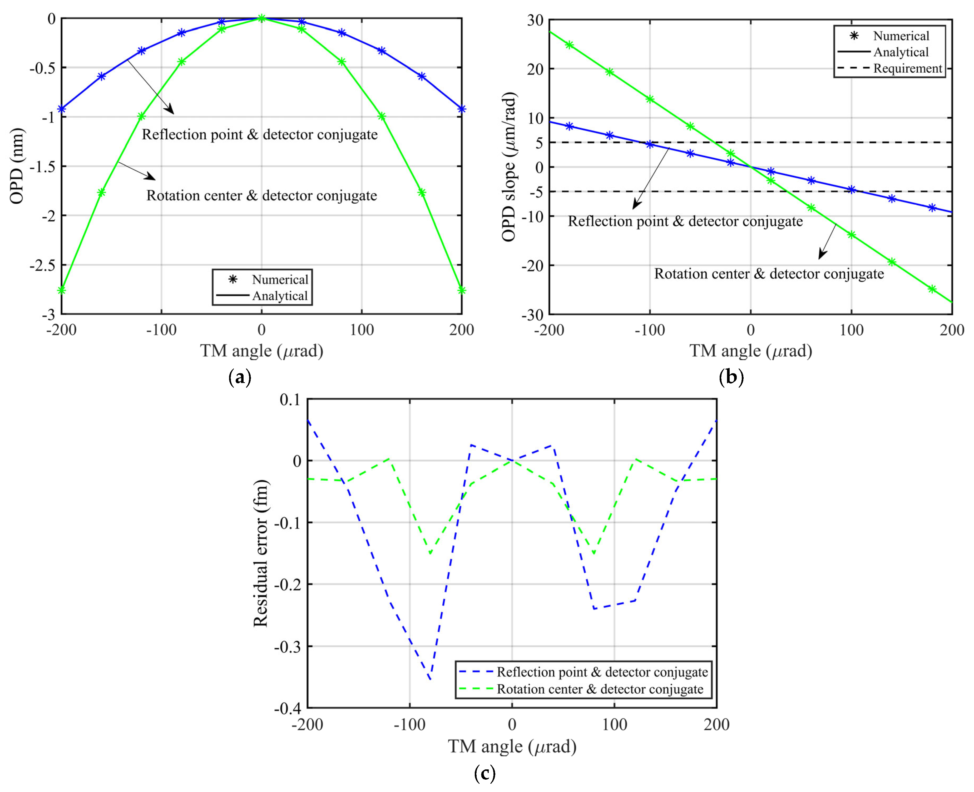
For the theoretical model in Section 3.2.1 and Section 3.2.2, the reflection point and the rotation center are conjugate with the center of the detector, respectively. The corresponding simulation results are illustrated in Figure 6, in which the analytical expressions and simulation results are represented by the solid lines and asterisks, respectively, and the residual errors are shown in Figure 6c. The numerical computations closely match the analytical expressions, with a residual error of less than 0.0004 pm, attributed to the high-order residues in Equations () and (). Nevertheless, as indicated in Figure 6b, both of the OPD slopes are far beyond the Taiji requirement.
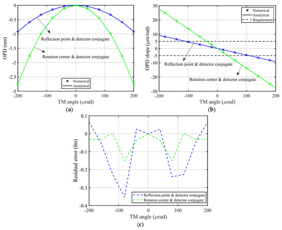
Figure 6.
Numerically and analytically computed OPD (a) and OPD slope (b) of the geometric TTL coupling model of the TM interferometer with the imaging system. The TTL coupling corresponding to the conjugation between the reflection point and the detector (), and that to the conjugation between the rotation center and the detector (), are represented by the blue and green lines (numerical: asterisks, analytical: solid line), respectively. The residual errors are shown in (c). The simulation results coincide with the analytic expressions, and the differences are due to the presence of the high-order residues in Equations () and ().
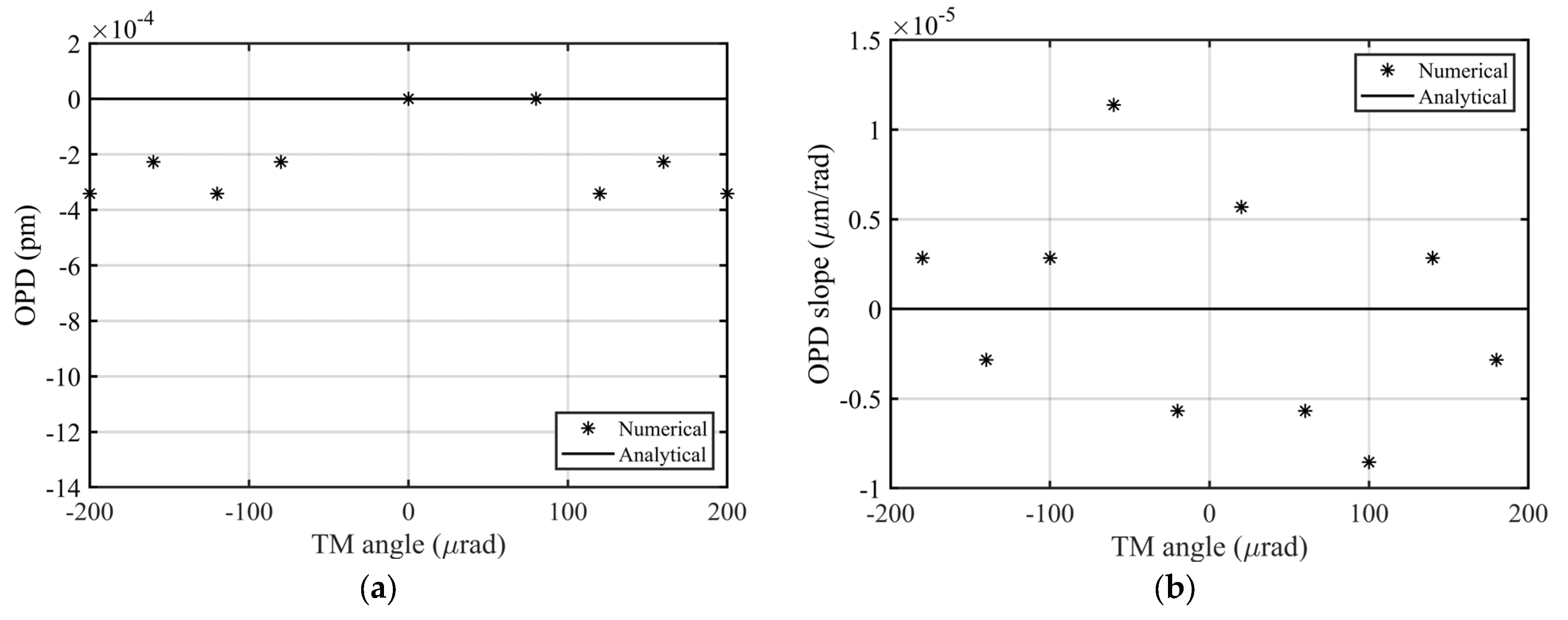
For the theoretical model in Section 3.3, i.e., the optimal conjugate relationship, the corresponding simulation results are shown in Figure 7, in which the analytical expressions and simulation results are represented by the solid lines and asterisks, respectively. We can find that the simulation results agree well with the analytic expressions, and the residual errors are less than 0.0004 pm, which comes from the presence of the high-order residues in Equations () and (). Obviously, the corresponding TTL coupling satisfies the Taiji requirement, and is even five orders of magnitude lower than the requirement.
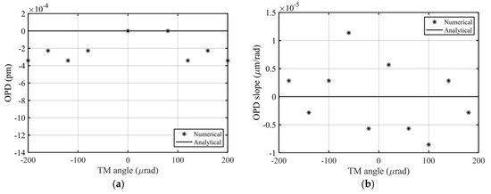
Figure 7.
Numerically and analytically computed OPD (a) and OPD slope (b) of the geometric TTL coupling model of the TM interferometer with the imaging system, under the condition of the optimal conjugation (). The analytical expressions and simulation results are represented by the black solid lines and the asterisks, respectively, and both of them match very well. The differences are due to the presence of the high-order residues in Equations (32) and (43).
Having obtained the optimal position of the imaging system for minimizing the geometric TTL coupling, we analyze the influence of the position deviation of the imaging system on the TTL coupling. This helps us to establish the requirement for the deployment of the imaging system. By intentionally deviating the nominal position of the imaging system in the optical model and measuring the resulting TTL coupling through numerical simulations, as illustrated in Figure 8, we can assess the influence of these deviations. The imaging system is considered as a whole to adjust the position.
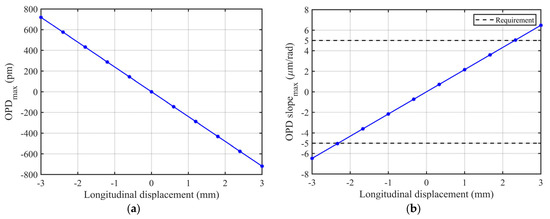
Figure 8.
The sensitivity analysis between the TTL coupling and optimal position offset by numerical simulation. The horizontal axis represents the longitudinal displacement of the optimal position for the imaging system as a whole, and the vertical axis represents the maximum offset of the corresponding OPD (a) and TTL coupling (b). It can be seen that the TTL coupling corresponding to displacement within ±2.33 mm can meet the requirement.
As shown in Figure 8, the imaging system can suppress the TTL coupling to the Taiji program’s requirement for the TM interferometer within a deviation of ±2.33 mm from the optimal position. This result provides valuable guidance for the design and adjustment of imaging systems in high precision interferometers.
5. Conclusions
In this paper, we present the analytical expression for the geometric TTL coupling in a TM interferometer equipped with an imaging system, and propose an optical configuration that theoretically suppresses TTL coupling when combined with post-processing. First, we investigate and demonstrate the geometric TTL coupling in the TM interferometer via numerical simulations. Then, we derive and examine the analytical expression of geometric TTL coupling with the imaging system, considering two typical conjugate relationships in realistic interferometer scenarios. Our findings indicate that TTL coupling in these two common cases significantly exceeds the Taiji program’s requirement. The first-order term cannot be eliminated through the introduction of the imaging system alone, but it can be mitigated by post-processing in orbit. Additionally, we deduce the optimal conjugate relationship, i.e., the nominal position of the imaging system, which nearly eliminates the TTL coupling. Finally, the theoretical analysis results regarding TTL coupling with the imaging system are confirmed through numerical simulations. We also conduct a sensitivity analysis between the TTL coupling and the optimal position offset, further validating the effectiveness of the optimal position of imaging system.
In summary, we have analyzed the mechanism of using an imaging system to suppress the geometric TTL coupling in a TM interferometer with alignment errors, and proposed a targeted method where the second-order term is suppressed through placing the imaging system in the optimal position or the tolerance range, and the first-order term is subtracted by in-orbit calibration. This method provides a theoretical basis for the design and adjustment of the optical layout in the LISA/Taiji program which calls for high precision laser interferometry. In fact, the non-geometric factors, including the wavefront properties, beam walk, diffraction and so on, will also affect the TTL coupling, which can be suppressed through an intentional position deviation of the detector and other means in a subsequent paper.
Author Contributions
Conceptualization, J.S. and S.W.; methodology, R.G.; software, W.T.; validation, J.S., S.W. and K.Q.; formal analysis, M.Z.; investigation, H.L.; resources, Z.L.; data curation, R.Y.; writing—original draft preparation, J.S.; writing—review and editing, J.S.; visualization, Z.L.; supervision, K.Q.; project administration, P.L.; funding acquisition, P.L. All authors have read and agreed to the published version of the manuscript.
Funding
This study was supported in part by grants from The National Key R&D Program of China (2022YFC2203702).
Institutional Review Board Statement
Not applicable.
Informed Consent Statement
Not applicable.
Data Availability Statement
Data are contained within the article.
Acknowledgments
Thanks for the help and technical support from other authors, and thanks for the financial support from the foundation.
Conflicts of Interest
The authors declare no conflicts of interest.
References
- Danzmann, K.; Rüdiger, A. LISA technology: Concept, status, prospects. Class. Quantum Grav. 2003, 20, S1–S9. [Google Scholar] [CrossRef]
- Jennrich, O. LISA technology and instrumentation. Class. Quantum Grav. 2009, 26, 153001. [Google Scholar] [CrossRef]
- Hu, W.-R.; Wu, Y.-L. The Taiji Program in Space for gravitational wave physics and the nature of gravity. Natl. Sci. Rev. 2017, 4, 685–686. [Google Scholar] [CrossRef]
- Luo, Z.; Guo, Z.; Jin, G.; Wu, Y.; Hu, W. A brief analysis to Taiji: Science and technology. Results Phys. 2020, 16, 102918. [Google Scholar] [CrossRef]
- Luo, Z.; Wang, Y.; Wu, Y.; Hu, W.; Jin, G. The Taiji program: A concise overview. Prog. Theor. Exp. Phys. 2021, 2021, 05A108. [Google Scholar] [CrossRef]
- Tao, W.; Deng, X.; Diao, Y.; Gao, R.; Qi, K.; Wang, S.; Luo, Z.; Sha, W.; Liu, H. Design and Construction of the Optical Bench Interferometer for the Taiji Program. Sensors 2023, 23, 9141. [Google Scholar] [CrossRef] [PubMed]
- Wang, Y.; Meng, L.; Xu, X.; Niu, Y.; Qi, K.; Bian, W.; Yang, Q.; Liu, H.; Jia, J.; Wang, J. Research on Semi-Physical Simulation Testing of Inter-Satellite Laser Interference in the China Taiji Space Gravitational Wave Detection Program. Appl. Sci. 2021, 11, 7872. [Google Scholar] [CrossRef]
- Gong, Y.; Luo, J.; Wang, B. Concepts and status of Chinese space gravitational wave detection projects. Nat. Astron. 2021, 5, 881–889. [Google Scholar] [CrossRef]
- Luo, J.; Chen, L.-S.; Duan, H.-Z.; Gong, Y.-G.; Hu, S.; Ji, J.; Liu, Q.; Mei, J.; Milyukov, V.; Sazhin, M.; et al. TianQin: A space-borne gravitational wave detector. Class. Quantum Grav. 2016, 33, 035010. [Google Scholar] [CrossRef]
- Armano, M.; Audley, H.; Auger, G.; Baird, J.T.; Bassan, M.; Binetruy, P.; Born, M.; Bortoluzzi, D.; Brandt, N.; Caleno, M.; et al. Sub-Femto-gFree Fall for Space-Based Gravitational Wave Observatories: LISA Pathfinder Results. Phys. Rev. Lett. 2016, 116, 231101. [Google Scholar] [CrossRef]
- Sasso, C.P.; Mana, G.; Mottini, S. Telescope jitters and phase noise in the LISA interferometer. Opt. Express 2019, 27, 16855–16870. [Google Scholar] [CrossRef] [PubMed]
- Tröbs, M.; Schuster, S.; Lieser, M.; Zwetz, M.; Chwalla, M.; Danzmann, K.; Barránco, G.F.; Fitzsimons, E.D.; Gerberding, O.; Heinzel, G.; et al. Reducing tilt-to-length coupling for the LISA test mass interferometer. Class. Quantum Grav. 2018, 35, 105001. [Google Scholar] [CrossRef]
- Wegener, H.; Müller, V.; Heinzel, G.; Misfeldt, M. Tilt-to-Length Coupling in the GRACE Follow-On Laser Ranging Interferometer. J. Spacecr. Rocket. 2020, 57, 1362–1372. [Google Scholar] [CrossRef]
- Chwalla, M.; Danzmann, K.; Fernández Barranco, G.; Fitzsimons, E.; Gerberding, O.; Heinzel, G.; Killow, C.J.; Lieser, M.; Perreur-Lloyd, M.; Robertson, D.; et al. Design and construction of an optical test bed for LISA imaging systems and tilt-to-length coupling. Class. Quantum Grav. 2016, 33, 245015. [Google Scholar] [CrossRef]
- Schuster, S. Tilt-to-Length Coupling and Diffraction Aspects in Satellite Interferometry. Ph.D. Thesis, Leibniz Universität, Hannover, Germany, 2017. [Google Scholar]
- Wanner, G. Complex Optical Systems in Space: Numerical Modelling of the Heterodyne Interferometry of LISA Pathfinder and LISA. Ph.D. Thesis, Leibniz Universität, Hannover, Germany, 2010. [Google Scholar]
- Lee, Y. Development of an Advanced Tilt Actuator for Tilt-to-Length Coupling Investigations. Ph.D. Thesis, Leibniz Universität, Hannover, Germany, 2021. [Google Scholar]
- Schuster, S.; Wanner, G.; Tröbs MHeinzel, G. Vanishing tilt-to-length coupling for a singular case in two-beam laser interferometers with Gaussian beams. Appl. Opt. 2015, 54, 1010–1014. [Google Scholar] [CrossRef]
- Schuster, S.; Tröbs, M.; Wanner GHeinzel, G. Experimental demonstration of reduced tilt-to-length coupling by a two-lens imaging system. Opt. Express 2016, 24, 10466–10475. [Google Scholar] [CrossRef] [PubMed]
- Chwalla, M.; Danzmann, K.; Alvarez, M.D.; Delgado, J.J.E.; Barranco, G.F.; Fitzsimons, E.; Gerberding, O.; Heinzel, G.; Killow, C.J.; Lieser, M.; et al. Optical Suppression of Tilt-to-Length Coupling in the LISA Long-Arm Interferometer. Phys. Rev. Appl. 2020, 14, 014030. [Google Scholar] [CrossRef]
- Paczkowski, S.; Giusteri, R.; Hewitson, M.; Karnesis, N.; Fitzsimons, E.D.; Wanner GHeinzel, G. Postprocessing subtraction of tilt-to-length noise in LISA. Phys. Rev. D 2022, 106, 042005. [Google Scholar] [CrossRef]
- Wanner, G.; Karnesis, N. Preliminary results on the suppression of sensing cross-talk in LISA Pathfinder. J. Phys. Conf. Ser. 2017, 840, 012043. [Google Scholar] [CrossRef]
- Hartig, M.-S. Tilt-To-Length Coupling in LISA Pathfinder: Model, Data Analysis and Take-Away Messages for LISA. Ph.D. Thesis, Leibniz Universität, Hannover, Germany, 2022. [Google Scholar]
- Hartig, M.-S.; Schuster, S.; Heinzel, G.; Wanner, G. Non-geometric tilt-to-length coupling in precision interferometry: Mechanisms and analytical descriptions. J. Opt. 2023, 25, 055601. [Google Scholar] [CrossRef]
- Hartig, M.-S.; Schuster, S.; Wanner, G. Geometric tilt-to-length coupling in precision interferometry: Mechanisms and analytical descriptions. J. Opt. 2022, 24, 065601. [Google Scholar] [CrossRef]
- Hartig, M.-S.; Wanner, G. Tilt-to-length coupling in LISA Pathfinder: Analytical modeling. Phys. Rev. D 2023, 108, 022008. [Google Scholar] [CrossRef]
- Zhao, Y.; Wang, Z.; Li, Y.; Fang, C.; Liu, H.; Gao, H. Method to Remove Tilt-to-Length Coupling Caused by Interference of Flat-Top Beam and Gaussian Beam. Appl. Sci. 2019, 9, 4112. [Google Scholar] [CrossRef]
- Born, M.; Wolf, E. Principles of Optics: Electromagnetic Theory of Propagation, Interference and Diffraction of Light, 7th ed.; Cambridge University Press: Cambridge, UK, 1999; pp. 160–175. [Google Scholar]

Disclaimer/Publisher’s Note: The statements, opinions and data contained in all publications are solely those of the individual author(s) and contributor(s) and not of MDPI and/or the editor(s). MDPI and/or the editor(s) disclaim responsibility for any injury to people or property resulting from any ideas, methods, instructions or products referred to in the content. |
© 2024 by the authors. Licensee MDPI, Basel, Switzerland. This article is an open access article distributed under the terms and conditions of the Creative Commons Attribution (CC BY) license (https://creativecommons.org/licenses/by/4.0/).