Power Testing of Aspheric Lenses Based on Transmission Phase Deflectometric Method

Abstract

Traditional methods for testing aspheric optical lenses struggle to achieve point-by-point testing across the full aperture of the lens. To facilitate the full-aperture, high-precision, and rapid testing of aspheric optical lenses, a power testing method of lenses based on the transmission phase deflectometric technique was employed. This method determines the phase deviation of light caused by the lens, thereby fitting the transmission wavefront and quickly detecting the power distribution information of the lens. This paper constructs a power testing model based on the phase deflectometric technique, proposes a calibration method that combines DLT (direct linear transformation) and pinhole models to reduce system errors, and combines phase extraction and wavefront fitting for experimental verification. The experimental results are compared with those obtained from the commercial visual lens mapper (VM-2000). The central errors of spherical power and cylindrical power are 1% and 0.7%, respectively. This provides a reliable method for the full-aperture, high-precision, and rapid testing of aspheric optical lenses.

1. Introduction

Traditional spherical lenses can no longer meet the needs of the glasses market, and lenses with higher degrees of freedom, such as aspheric lenses, are needed. Aspheric lenses offer designers enhanced flexibility compared to traditional spherical lenses, enabling significant improvements in the optical performance metrics of optical systems, particularly in correcting aberrations. The high-precision measurement of aspheric optical lens parameters serves as a critical basis for evaluating overall lens performance. Therefore, full-aperture power parameter testing of aspheric lenses is particularly important. Traditional power testing methods use a focimeter [1], which only measures average power and is suitable for spherical lenses and some aspheric lenses. The power parameters of aspheric optical lenses are generally calculated from the transmission wavefront of the lens. Current transmission wavefront testing methods include contact methods [2,3,4], such as three-coordinate measuring instruments and probe contour meters. Contact methods can scratch the surface of the lens, causing damage and disrupting the continuity of the surface.

There are also non-contact methods, such as laser interferometry [5], the Hartmann map method [6], the reflective phase deflection method [7], the transmission phase deflection method [8,9], holographic computational interferometry [10], the Moire deviation method [11], and the Ronchi grating method [12]. Laser interferometry primarily employs instruments like Twyman–Green and Fizeau interferometers [13] for measurements, utilizing phase shifting interferometry principles to capture real-time interference patterns with specific phase differences. This method offers high precision and wide applicability, albeit at higher costs. The core of the Hartmann map method is a microlens array, which cannot accommodate high-resolution and large-range curvature measurements. The reflective phase deviation method requires one side to be painted black during testing, which damages the continuity and integrity of the lens surface. In holographic computational interferometry, the manufacture of the CGH is complex, the accuracy of installation and adjustment is low, it is not universal, and it is not suitable for real-time factory testing and mass production. The Moire deflection method and the Ronchi grating method have similar principles and suffer from long sampling periods, relatively long measurement times, and high-precision requirements for gratings.

Aiming to resolve the problems of the above series of detection methods in order to realize the rapid detection of the full aperture and large curvature range of lenses, this paper reports a transmissive phase deflection method, which further solves the power of the lens by collecting and solving the phase change due to the lens and fitting the wavefront based on Zernike polynomials. The proposed method has the advantages of environmental insensitivity, a simple structure, and fast detection speed, which can realize the full-aperture, large curvature range, and high-precision detection of optical aspheric lenses, and can also be used for the detection of other transmissive optical elements.

2. Materials and Methods

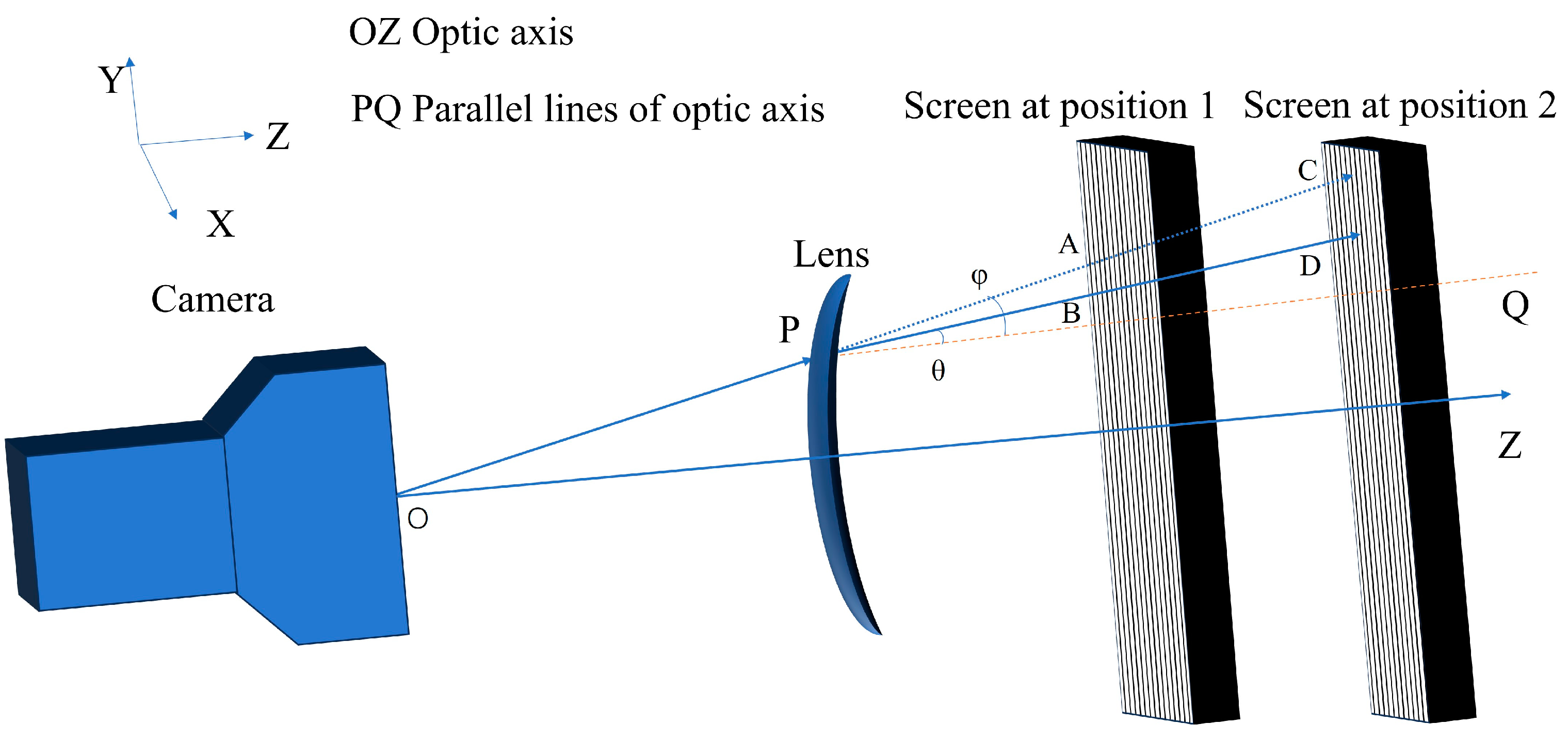
2.1. Principle of Transmission Phase Deflection

The principle of the transmission phase deflectometric method is shown in Figure 1. The entire testing system consists of a camera, a lens, and a screen. The camera captures the periodic in the horizontal direction and vertical direction sinusoidal fringes patterns generated by the screen, with a spatial frequency of fringes of 0.0862 mm⁻¹. The light path is reversible, and the O of the camera is considered the light source. When the lens is not added, the light propagates along the direction of OA and intersects with the screen at positions 1 and 2 at points A and C. After the lens is added, the light is deflected (e.g., at point P) and continues to propagate along the direction of PB and intersects with the screen at positions 1 and 2 at points B and D. The distance between the two screens is d; thus, the following relationship is established:

$$\begin{array}{c}\tan {\phi }_x={\displaystyle \frac{C_x-A_x}{d}}\\ \tan {\theta }_x={\displaystyle \frac{D_x-B_x}{d}}\end{array}$$

(1)

$$\{\begin{array}{c}\tan {\phi }_y={\displaystyle \frac{C_y-A_y}{d}}\\ \tan {\theta }_y={\displaystyle \frac{D_y-B_y}{d}}\end{array}$$

(2)

where φ and θ are the angles between the un-deflected ray AC and the deflected ray BD and the optical axis, respectively.

The changes in the slope of the wavefront at point P in the x and y directions are, respectively, as follows:

$$\{\begin{array}{c}slop{e}_x=\tan ({\phi }_x-{\theta }_x)\\ slop{e}_y=\tan ({\phi }_y-{\theta }_y)\end{array}$$

(3)

The phase information graph on the screen is captured, and the phase shift method and phase unwrapping are used to solve the phase diagram carrying the light deviation information of the lens, and the corresponding phase information is obtained. Combined with the calibration part of the system, the transmission wavefront slope of all points in the optical area is integrated and reconstructed, and the complete transmission wavefront is fitted. Based on the transmission wavefront, optical parameters such as power are calculated.

2.2. System Calibration and Phase Information Extraction

System calibration is divided into internal and external parameters. The technology for calibrating the camera’s internal parameters is well developed, and common calibration methods include checkerboard calibration and Tsai calibration [14]. The calibration of external parameters is usually based on the actual system to establish a calibration method, and finally, all components of the system are unified under the world coordinate system. In order to minimize the system’s calibration error, this paper proposes a calibration method which is DLT [15] (direct linear transformation) combined with a pinhole imaging model to obtain an external reference matrix.

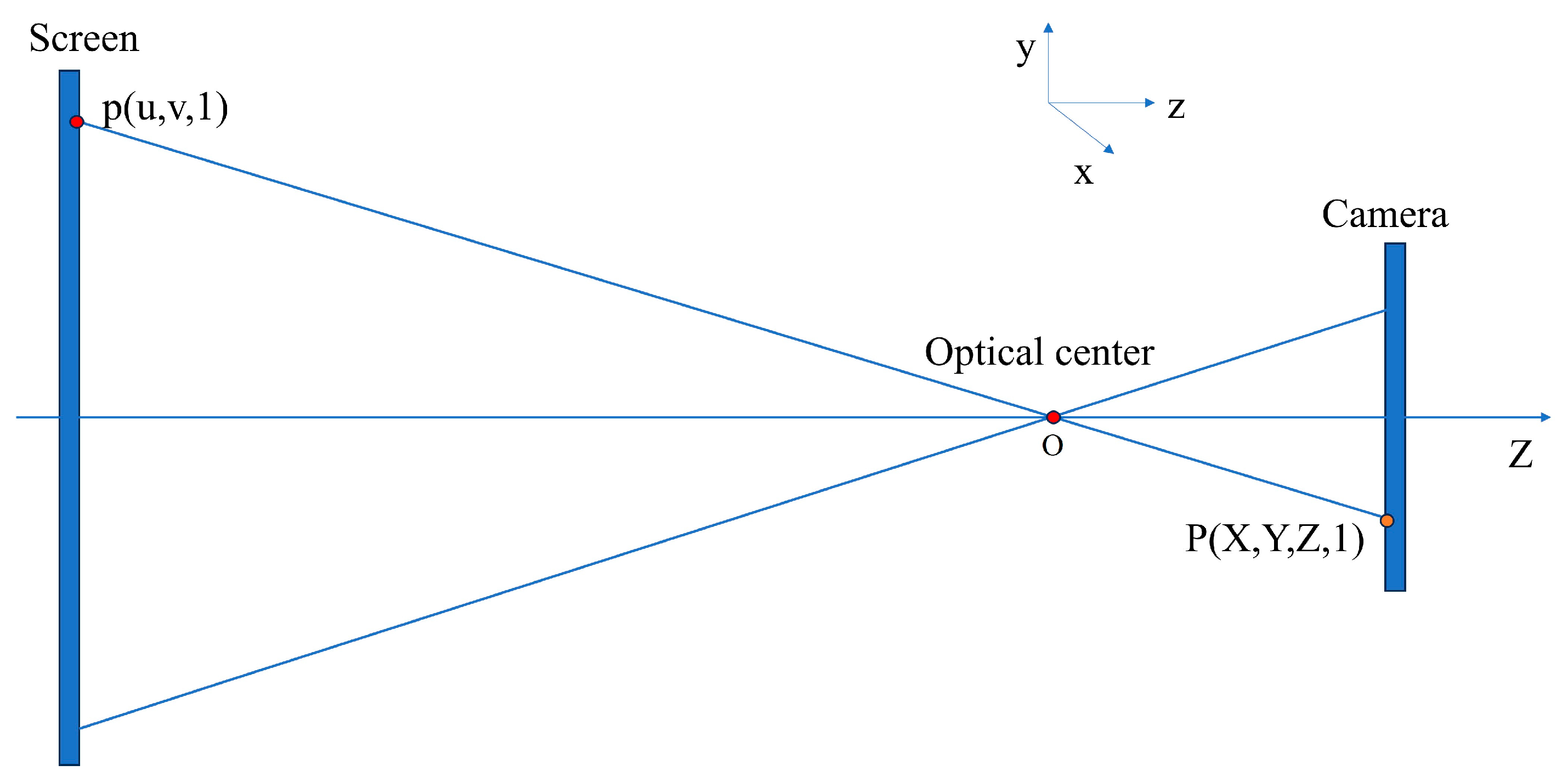
2.2.1. External Parameter Calibration

External parameter calibration is used to determine the relationship matrix between the screen pixel coordinate system and the camera coordinate system, thereby unifying the coordinate system of the entire system. This paper employs the pinhole imaging principle, taking the camera’s optical center as the pinhole, establishing a pinhole model between the camera coordinate system and the screen coordinate system, and implementing external parameter calibration with the DLT algorithm. The schematic diagram is shown in Figure 2.

In the camera coordinate system, a feature point on the camera image plane, for example, point P, whose coordinates are P(X,Y,Z,1), and the pixel coordinates of the corresponding feature point p in the screen coordinate system, which are p(u,v,1), are known by the imaging principle to have the following projection relationship:

$$Sp=[Rt]P$$

(4)

where S is the scale factor, R is the rotation matrix, and t is the translation matrix. We can expand this to obtain Equation (5):

$$S\left(\begin{array}{c}u\\ v\\ 1\end{array}\right)=\left(\begin{array}{cccc}{R}_{11}& R_{12}& R_{13}& t_1\\ R_{21}& R_{22}& R_{23}& t_2\\ R_{31}& R_{32}& R_{33}& t_3\end{array}\right)\left(\begin{array}{c}X\\ Y\\ Z\\ 1\end{array}\right)$$

(5)

We can expand this by each row as follows:

$$\{\begin{array}{l}Su=R_{11}X+R_{12}Y+R_{13}Z+t_1\\ Sv=R_{21}X+R_{22}Y+R_{23}Z+t_2\\ S=R_{31}X+R_{32}Y+R_{33}Z+t_3\end{array}$$

(6)

A point pair can provide two equations, and there are a total of 12 unknowns in the [Rt] matrix, so the number of point pairs n ≥ 6 is required. We can normalize the coordinates of the point pairs and solve the following overdetermined equations to obtain the [Rt] matrix.

$$\left(\begin{array}{ccc}-P^{\prime }& 0& u{P}^{\prime }\\ 0& -P^{\prime }& v{P}^{\prime }\end{array}\right)h=0$$

(7)

where $h=\left(\begin{array}{cccccccccccc}{R}_{11}& R_{12}& R_{13}& R_{21}& R_{22}& R_{23}& R_{31}& R_{32}& R_{33}& t_1& t_2& t_3\end{array}\right)$; the solved [Rt] matrix is the external parameter matrix.

2.2.2. Phase Information Extraction

The phase shift method is used to extract the wrapped phase of the acquired fringe image. Among them, the five-step phase shift method has the advantage of being insensitive to the light in the environment; so, the five-step phase shift method was used to extract the wrapped phase. The five-step phase shifting method aims to evenly collect five intensity maps of the sinusoidal fringe with the same period and a phase difference of π/2 on the time axis. The intensity is denoted as I(x,y), the phase coordinate is φ(x,y), and the initial phases of the five generated sinusoidal phase diagrams are 0, π/2, π, 3π/2, and 2π:

$$\{\begin{array}{c}{I}_1(x,y)=I_B+I_M(x,y)\cos [\phi (x,y)]\\ I_2(x,y)=I_B+I_M(x,y)\cos [\phi (x,y)+{\displaystyle \frac{\pi }{2}}]\\ I_3(x,y)=I_B+I_M(x,y)\cos [\phi (x,y)+\pi ]\\ I_4(x,y)=I_B+I_M(x,y)\cos [\phi (x,y)+{\displaystyle \frac{3\pi }{2}}]\\ I_5(x,y)=I_B+I_M(x,y)\cos [\phi (x,y)+2\pi ]\end{array}$$

(8)

where I_B is the background light intensity and I_M is the modulated light intensity. Equation (9) can be rearranged to obtain

$$\phi (x,y)={\tan }^{-1}{\displaystyle \frac{2(I_2-I_4)}{I_1+I_5-2I_3}}.$$

(9)

The amplitude of the phase φ(x,y) is between −π/2 and π/2, which is the wrapped phase. Further, the true phase is obtained by solving the phase using discrete cosine varying least squares. This method is a phase unwrapping algorithm based on the minimum norm method [16], that is, to find the solution in the sense of the minimum L^p norm of the phase difference between adjacent pixels of the unwrapped phase φ and the wrapped phase φ, thereby obtaining the real phase.

2.3. Transmission Wavefront Fitting and Related Parameter Solving

2.3.1. Transmission Wavefront Fitting

The unwrapped phase coordinates φ(x,y) are converted into screen pixel coordinates p(u,v,1) [17]. Combining Equations (1)–(3) and (9), the slopes slope_x and slope_y in the x and y directions of a point on the surface of the lens can be solved. The mode method based on Zernike polynomials was used for the fitting of the transmission wavefront. The transmission wavefront can be represented as follows:

$$W(x,y)={\displaystyle \sum _{i=0}^n{K}_i{Z}_I(x,y)}$$

(10)

Then, the slope of the transmission wavefront in the x and y directions can be represented as follows:

$$\{\begin{array}{c}{\displaystyle \frac{\partial W(x,y)}{\partial x}}={\displaystyle \sum _{i=0}^n{K}_i\frac{\partial Z(x,y)}{\partial x}}\\ {\displaystyle \frac{\partial W(x,y)}{\partial y}}={\displaystyle \sum _{i=0}^n{K}_i\frac{\partial Z(x,y)}{\partial y}}\end{array}$$

(11)

By solving the above overdetermined equations, the coefficients K_i of the Zernike polynomial can be obtained. We substitute this into Equation (11) to fit the wavefront.

2.3.2. Mathematical Modeling of Power

The transmitted wavefront is solved from the above equation as W(x,y). According to the definition of curvature in differential geometry [18], the coefficients of the first surface equation and the coefficients of the second surface equation at a point on the surface are solved. The coefficients of the first surface are related to the first derivative of the transmission wavefront, and those of the second surface equation are related to the second derivative of the transmission wavefront. The coefficients and the principal curvatures λ_max and λ_min have the following relationship:

$$\left|\begin{array}{cc}L-\lambda E& M-\lambda F\\ M-\lambda F& N-\lambda G\end{array}\right|=0$$

(12)

where E, F, and G are first surface equation coefficients and M, L, and N second surface equation coefficients.

The principal curvatures λ_max and λ_min at that point can be obtained, and the spherical power and cylindrical power corresponding to that point are calculated as follows:

$$\{\begin{array}{l}S={\displaystyle \frac{{\lambda }_{max}+{\lambda }_{min}}{2}}\\ C=\left|\begin{array}{c}{\lambda }_{max}-{\lambda }_{min}\end{array}\right|\end{array}$$

(13)

where S is the spherical power of the lens and C is the cylindrical power of the lens.

3. Results

3.1. Experimental Verification

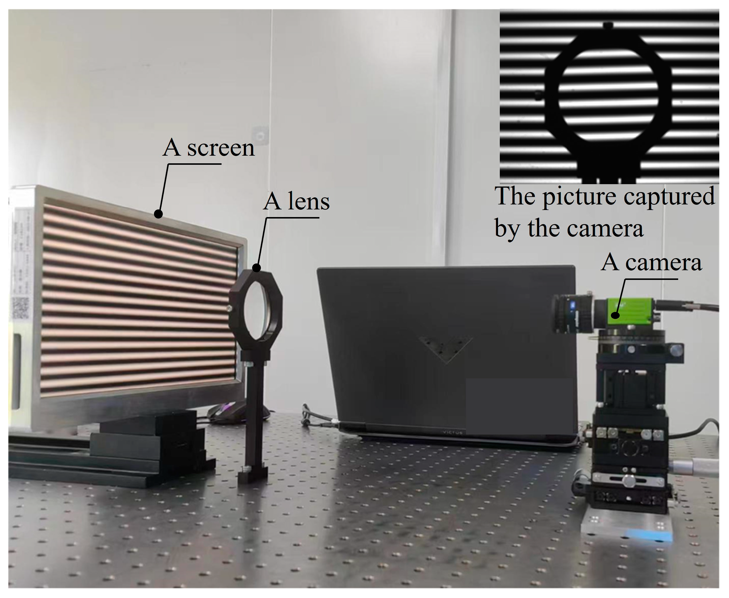
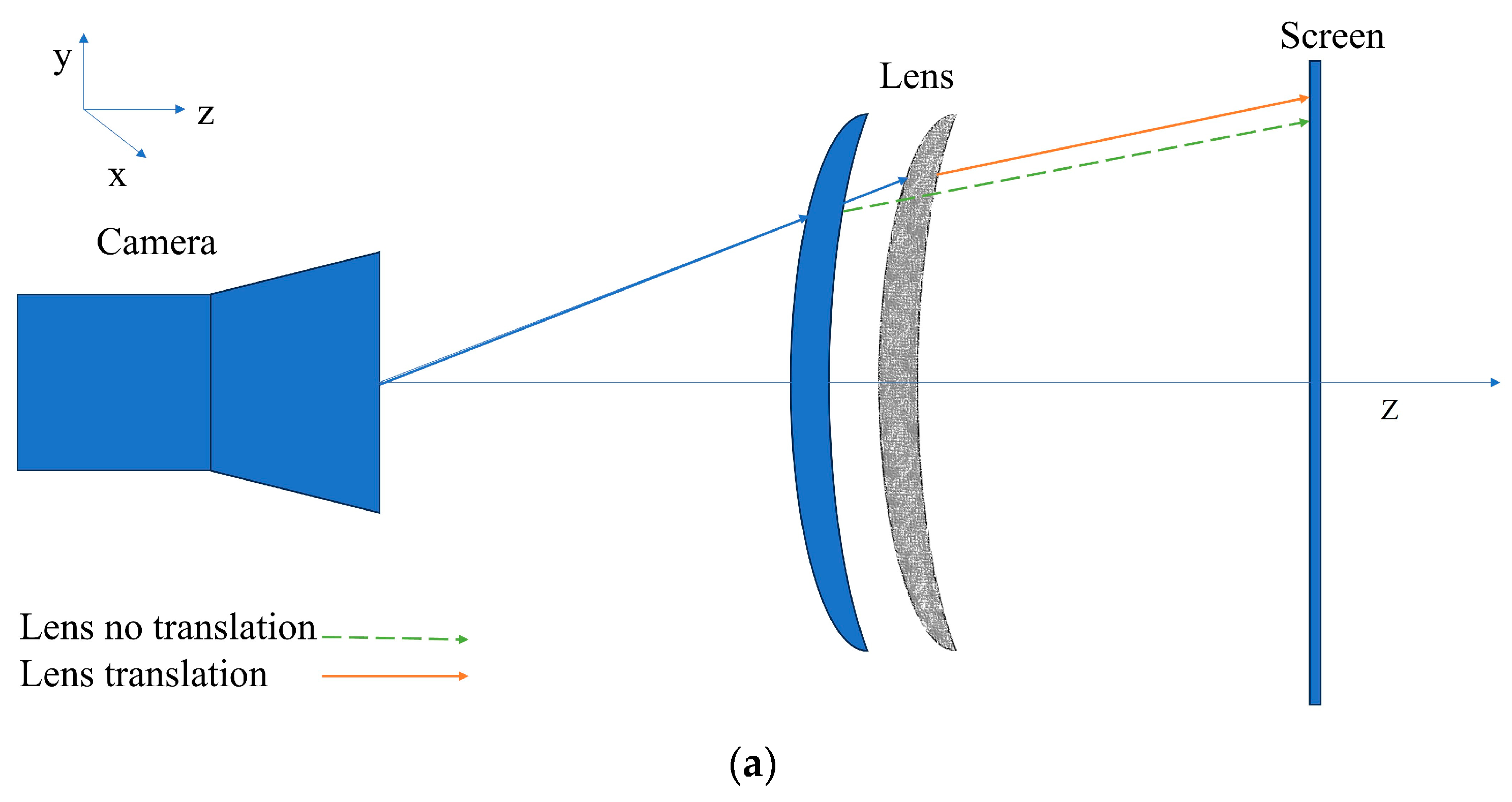
3.1.1. Experimental Setup

In order to verify the accuracy of the refractive power distribution of aspheric lenses detected by the transmission phase deflectometric method, an experimental optical path (Figure 3) was set up according to the principle (Figure 1). An ON-Semiconductor GO_5000 image sensor (resolution: 2560 × 2048, pixel size: 5 μm, image plane size: 16 mm, frame rate: 60 fps) shown in Figure 3 was adopted as the photoreceptor. This sensor has high quantum efficiency. The camera lens uses a 25 mm fixed-focus lens from AZURE company which located in Fuzhou, China; the screen uses a Dell C1422H model 14.0 in. monitor, with a pixel size of 0.1611 mm × 0.1611 mm.

Five sinusoidal fringe images of the same period in the horizontal and vertical directions were generated on the screen. The focal length and aperture of the camera were adjusted so that the camera could capture clear pictures at a distance of both screen position 1 and screen position 2. Next, the adjusted focal depth and aperture were fixed and the camera was calibrated with internal parameters. The internal reference matrix was obtained by using the checkerboard calibration method based on MATLAB R2020b software. A total of 50 checkerboard images with corner point distances of 6.444 mm at different positions were used to obtain the internal reference matrix. The calibration results show that the calibration error of the distance between screen position 1 (L1) and screen position 2 (L2) is 1 mm. The accuracy of this error meets the experimental requirements. The feature point maps of 10 × 20 with the same spacing are used to obtain the external reference matrix based on our proposed external reference calibration method, which adjusts the optical axis of the camera to be perpendicular to the plane of the screen, captures the feature point maps when the spacing between all of the feature points of the image plane is equal, and solves the external reference matrix.

The phase maps in the horizontal and vertical directions were collected at screen position 1 and screen position 2 with and without a lens added, respectively, and the phase was solved by Equations (8) and (9). The phase expansion in the x and y directions is shown in Figure 4 (Figure 4a: phase in the x direction; Figure 4b: phase in the y direction). Then, slope_x and slope_y in the x and y directions were solved by combining them with the system’s calibration, and the transmission wavefront was fitted based on the Zernike polynomials; the lens refractive index distributions (spherical power and cylindrical power) were solved based on the power parameter calculation model.

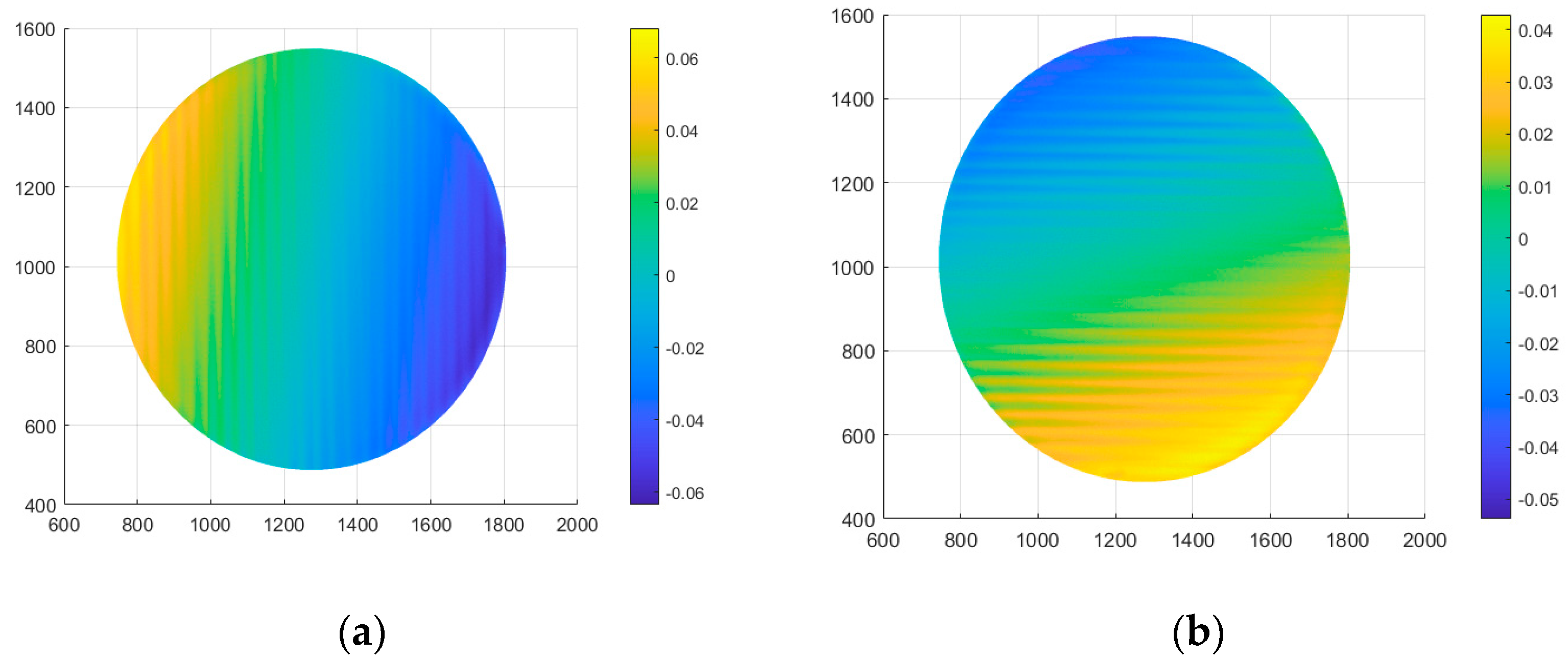
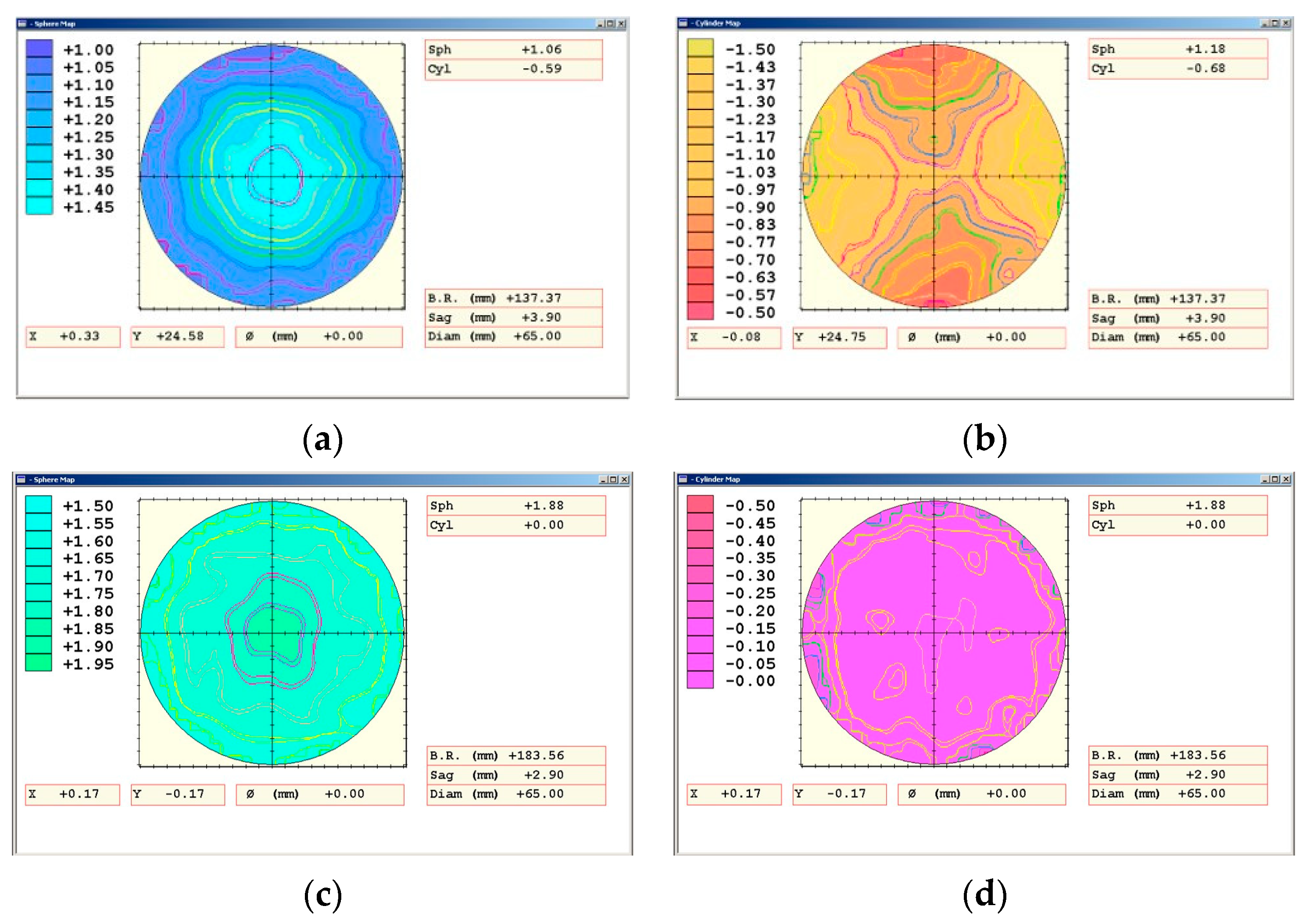
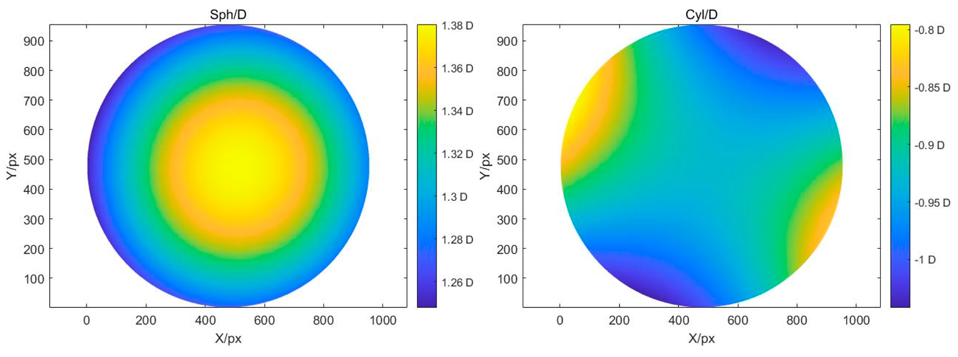
3.1.2. Experimental Results

An aspheric lens (diameter: 65 mm; spherical power: +1 D; cylindrical power: −1 D) was tested based on the constructed transmission phase deflection system. The distance between the lens and the screen was set to 60 mm. The test results are shown in Figure 5 (Figure 5a,b). The center value of the spherical power map (Figure 5a) is 1.45 D, and the edge value of the spherical power map is 1.34 D. From the power map, it can be seen that there is a decreasing trend from the center to the edge, which is in line with the design principle of aspheric lenses. The maximum and minimum values of the edge of the cylindrical power map (Figure 5b) are −0.85 D and −1.10 D. In order to verify the accuracy of the present system, the VM-2000 commercial visual lens mapper from VISIONIX, Israel, was used to carry out the comparison experiments. The test results are shown in Figure 6 (Figure 6a,b). The center and edge values of the spherical power map (Figure 6a) are 1.46 D and −1.34 D, respectively. The difference between their center and edge values is 0.01 D and 0.34 D, respectively. Similarly, the center and edge values of the cylindrical power map maintain high accuracy, with error values of 0.03 D and 0.3 D, respectively. From the comparison results, it can be seen that the transmissive phase deflection system has high accuracy in the testing of the power of lenses. To further validate the accuracy of our proposed measurement technique, another aspheric lens (spherical power: +2 D; cylindrical power: 0 D) was tested based on the constructed transmission phase deflection system. The test results are shown in Figure 5 (Figure 5c,d). Similarly, in order to verify the accuracy of the present system, the VM-2000 commercial visual lens mapper from VISIONIX, Tel-Aviv, Israel, was used to carry out the comparison experiments. The test results are shown in Figure 6 (Figure 6c,d). From the comparison results, it can be seen that the transmissive phase deflection system maintains the same high accuracy in the testing of the power of lenses.

4. Discussion

In the experiment, the camera’s optical center is regarded as an ideal pinhole, the camera’s image plane and the screen are regarded as the image plane and object plane in the experimental system, respectively, and the screen emits parallel light, which is collected by the camera’s image plane through the pinhole. When the lens is not added, the acquired phase map is used as the reference phase; after the lens is added, the acquired phase map is the phase after the lens is deflected, and the deflection between the two is the transmitted wavefront information of the lens itself [19]. In the experiment, the camera’s optical center cannot be an ideal pinhole, and the lens system of the camera lens will introduce aberrations, mainly distortion. This system uses a distortion-free lens, so the distortion introduced by the camera lens is basically eliminated. When there is a large difference in ambient light intensity, it will affect the detection accuracy. The detection is generally conducted indoors with low light intensity. Moreover, the phase shifting method of this system is very insensitive to the light in the environment, which to a certain extent reduces the error caused by ambient light. The main sources of error in this system are the calibration of screen positions L1 and L2 and the tilt of the lens. The perpendicularity of the screen to the system’s optical axis is guaranteed by the workpiece, with an accuracy of 0.01 mm. In addition to the screen’s position, the offset position of the lens under test in the system is also a source of error, as shown in Figure 7. The solid lines in the figure represent the light rays when the lens is offset, and the dashed lines represent the light rays when the lens is in the correct position.

In the experiment, translation, eccentricity, and tilting of the lens will change the path of the original light ray, thus introducing errors. The experimental system remains unchanged and a translation, an eccentricity of 5 mm, and a tilt of 3° are introduced at the original position of the lens; the experimental results are shown in Figure 7a, Figure 7b, and Figure 7c, respectively. The corresponding power maps of the lens results are shown in Figure 8, Figure 9, and Figure 10, respectively. Compared with the experimental results without the introduction of errors, when the lens is translated, the center of the spherical power map is 1.52 D, with a difference of 0.04 D, and the center of the cylindrical power map diagram is −1.05 D, with a difference of 0.05 D. When the lens is eccentric, the center of the spherical power map is 1.58 D, which differs by 0.10 D; the center of the cylindrical power map is −1.06 D, which differs by 0.06 D. When the lens is tilted, the center values of the spherical and cylindrical power are 1.38 D and −0.95 D, respectively, and the difference between their center values is 0.08 D and 0.05 D, respectively. In conclusion, when the lens is translated, eccentric, and tilted, the average error in the center of the spherical and cylindrical power maps is within 8%, and there is no large error in the values of the edge regions. In addition, the shapes of the spherical power maps and cylindrical power maps are almost the same without much variation.

5. Conclusions

This paper presents a measurement of the power of lenses based on the transmissive phase deflection method, along with a calibration technique integrating direct linear transformation (DLT) with a pinhole model. The proposed calibration method not only simplifies operation but also significantly reduces system errors. The experimental results demonstrate that our constructed detection system achieves comparable accuracy to the commercial visual lens mapper (VM-2000). This offers a reliable solution for the full-aperture, high-precision, and rapid testing of aspherical lenses.

References

1. Park, J.; Chen, L.; Wang, Q.; Griesmann, U. Modified Roberts-Langenbeck test for measuring thickness and refractive index variation of silicon wafers. Opt. Express 2012, 20, 20078–20089. [Google Scholar] [CrossRef] [PubMed]
2. Mohtashami, V.; Shishegar, A.A. Modified wavefront decomposition method for fast and accurate ray-tracing simulation. IET Microw. IET Microw. Antennas Propag. 2012, 6, 295–304. [Google Scholar] [CrossRef]
3. Xiao, Y.; Zhou, L.; Chen, W. Wavefront control through multi-layer scattering media using single-pixel detector for high-PSNR optical transmission. Opt. Lasers Eng. 2021, 139, 106453. [Google Scholar] [CrossRef]
4. He, H.; Wong, K.S. An improved wavefront determination method based on phase conjugation for imaging through thin scattering medium. J. Opt. 2016, 18, 085604. [Google Scholar] [CrossRef]
5. Kim, S.; Jeon, J.; Kim, Y.; Sugita, N.; Mitsuishi, M. Design and Assessment of Phase-Shifting Algorithms in Optical Interferometer. Int. J. Precis. Eng. Manuf. Green Technol. 2023, 10, 611–634. [Google Scholar] [CrossRef]
6. Brooks, A.F.; Kelly, T.-L.; Veitch, P.J.; Munch, J. Ultra-sensitive wavefront measurement using a Hartmann sensor. Opt. Express 2007, 15, 10370–10375. [Google Scholar] [CrossRef] [PubMed]
7. Canabal, H.C. Automatic wavefront measurement technique using a computer display and a charge-coupled device camera. Opt. Eng. 2002, 41, 822–826. [Google Scholar] [CrossRef]
8. Vargas, J.; Gómez-Pedrero, J.A.; Alonso, J.; Quiroga, J.A. Deflectometric method for the measurement of user power for ophthalmic lenses. Opt. Dep. 2010, 17, 5125–5132. [Google Scholar] [CrossRef]
9. Markus, C.K.; Jurgen, K.; Gerd, H. Phase measuring deflectometry: A new approach to measure specular free-form surfaces. Proc. SPIE 2004, 5457, 366–376. [Google Scholar]
10. Lanen, T.A.W.M.; Bakker, P.G.; Bryanston-Cross, P.J. Digital holographic interferometry in high-speed flow research. Exp. Fluids 1992, 13, 56–62. [Google Scholar] [CrossRef]
11. Wang, Q.; Yu, J.; Chen, H. Measurement of lenses’ power based on moire deflection technology. In Proceedings of the 3rd International Symposium on Advanced Optical Manufacturing and Testing Technologies: Optical Test and Measurement Technology and Equipment, Chengdu, China, 8–12 July 2007; Volume 6723, pp. 118–123. [Google Scholar]
12. Arasa, J.; Royo, S.; Tomàs, N. Simple method for improving the sampling in profile measurements by use of the Ronchi test. Appl. Opt. 2000, 39, 4529–4534. [Google Scholar] [CrossRef] [PubMed]
13. Ichihara, Y. Evolution of Wavefront Metrology Enabling Development of High-Resolution Optical Systems. Opt. Rev. 2014, 21, 833–838. [Google Scholar] [CrossRef]
14. Chang, G. Surfing the metasurface: A conversation with Din Ping Tsai. Adv. Photonics 2023, 5, 060502. [Google Scholar] [CrossRef]
15. Abdel-Aziz, Y.; Karara, H. Direct linear transformation from comparator coordinates into object space coordinates in close-range photogrammetry. Photogramm. Eng. Remote Sens. 2015, 81, 103–107. [Google Scholar] [CrossRef]
16. Pepe, A.; Manunta, M.; Mazzarella, G.; Lanari, R. A Space-Time Minimum Cost Flow Phase Unwrapping Algorithm for the Generation of Persistent Scatterers Deformation Time-Series. In Proceedings of the 2007 IEEE International Geoscience and Remote Sensing Symposium, Barcelona, Spain, 23–28 July 2007; pp. 5285–5288. [Google Scholar]
17. Flores, J.L.; Bravo-Medina, B.; Ferrari, J.A. One-frame two-dimensional deflectometry for phase retrieval by addition of orthogonal fringe patterns. Appl. Opt. 2013, 52, 6537–6542. [Google Scholar] [CrossRef] [PubMed]
18. Harris, W.F. Calculation and least-squares estimation of surface curvature and dioptric power from meridional measurements. Ophthalmic Physiol. Opt. 1992, 12, 58–64. [Google Scholar] [PubMed]
19. Wang, D.; Xu, P.; Wu, Z.; Fu, X.; Wu, R.; Kong, M.; Liang, J.; Zhang, B.; Liang, R. Simultaneous multisurface measurement of freeform refractive optics based on computer-aided deflectometry. Optica 2020, 7, 1056–1064. [Google Scholar] [CrossRef]
Figure 1. A schematic diagram of the principle of the transmitted phase deflectometric system for testing the lens refractive power.
Photonics 11 00756 g001
Figure 2. A schematic diagram of the DLT principle used to obtain the external reference matrix.
Photonics 11 00756 g002
Figure 3. A picture of the experimental setup of the transmission phase deflection measurement system.
Photonics 11 00756 g003
Figure 4. Phase map differences obtained with fringe orientations: (a) x direction; (b) y direction.
Photonics 11 00756 g004
Figure 5. (a,c) The spherical power map of the design theoretical value 1 D and 2 D lenses, respectively, obtained using our technique for the lens; (b,d) the cylindrical power map of the design theoretical value −1 D and 0 D lenses, respectively, using our technique.
Photonics 11 00756 g005
Figure 6. (a,c) The spherical power map of the design theoretical value 1 D and 2 D lenses, respectively, obtained using the commercial profilometer VM-2500; (b,d) the cylindrical power map of the design theoretical value −1 D and 0 D lenses, obtained using the commercial profilometer VM-2500 from ANCIENTO in Liaoning, China.
Photonics 11 00756 g006
Figure 7. A schematic diagram of the error optical path introduced when the lens placement is (a) translational, (b) eccentric, and (c) tilted.
Photonics 11 00756 g007aPhotonics 11 00756 g007b
Figure 8. The power map obtained when the lens was translated (left: spherical power map; right: cylindrical power map).
Photonics 11 00756 g008
Figure 9. The power map obtained when the lens was placed 5 mm off-center (left: spherical power map; right: cylindric power map).
Photonics 11 00756 g009
Figure 10. The power map obtained when the lens was placed at tilt of 3° (left: spherical power map; right: cylindrical power map).
Photonics 11 00756 g010
Disclaimer/Publisher’s Note: The statements, opinions and data contained in all publications are solely those of the individual author(s) and contributor(s) and not of MDPI and/or the editor(s). MDPI and/or the editor(s) disclaim responsibility for any injury to people or property resulting from any ideas, methods, instructions or products referred to in the content.