Article

Theoretical Investigation of the Influence of Correlated Electric Fields on Wavefront Shaping

1
Institut für Lasertechnologien in der Medizin und Meßtechnik an der Universität Ulm, D-89081 Ulm, Germany
2
Faculty of Natural Sciences, Ulm University, D-89081 Ulm, Germany
*
Author to whom correspondence should be addressed.
Photonics 2024, 11(9), 797; https://doi.org/10.3390/photonics11090797
Submission received: 26 June 2024 / Revised: 15 August 2024 / Accepted: 22 August 2024 / Published: 27 August 2024
(This article belongs to the Special Issue Photonics: 10th Anniversary)

Abstract

:
Wavefront shaping is a well-known method of restoring a focus deep within scattering media by manipulating the incident light. However, the achievable focus enhancement depends on and is limited by the optical and geometrical properties of the medium. These properties contribute to the number of linearly independent transmission channels for light propagating through the turbid medium. Correlations occur when the number of incident waves coupled into the scattering medium exceeds this finite number of transmission channels. This paper investigates the wavefront shaping of such correlated electric fields. The influence of the observed correlations persists even though the average electric field distribution at positions in the focal plane follows a circular complex Gaussian. We show that correlations of the transmitted electric fields reduce the achievable intensity enhancement, even deep in the turbid medium. The investigations are carried out using a Monte Carlo algorithm. It is based on the speckle statistics of independent waves and introduces correlations of neighbouring electric fields via a Cholesky decomposition of the covariance matrix. Additional investigations include scenarios where the electric fields are not completely randomized, such as for ballistic or insufficiently scattered light. Significant contributions from such little-scattered light are observed to reduce the intensity enhancement further. Data from simulations solving Maxwell’s equations are compared with the results obtained from the Monte Carlo simulations for validation throughout this paper.

1. Introduction

Light propagating through a turbid medium is influenced by scattering and absorption. The increasing loss of directionality and intensity with increasing penetration depth limits many optical methods to shallow depths. Enhancing the imaging depth via recovery of a distorted focus, wavefront shaping (WFS) exploits the linear and deterministic behaviour of scattering present in static media. Precise manipulation of the amplitude and the phase of the incident light forces constructive interference inside or behind a turbid medium [1,2,3,4]. Controlling electric fields propagating through disordered media and especially their correlations [5,6], utilizing, e.g., transmission eigenchannels [7,8,9,10,11,12,13] and scattering invariant modes [14] allows further improvements in light transport and thus in the capability of WFS. These correlations have practical applications in wide-field and hidden-object imaging [15,16].
Correlations in the transmission channels of disordered media lead to the robustness of the transmitted speckle pattern to changes in the incident field. This phenomenon is called memory effect (ME) [17,18,19,20]. The influence of correlations is particularly apparent when the number of input modes is greater than the number of transmission modes [1,21]. A direct consequence of this can, e.g., be seen in the deviation of the achievable focus enhancement from the theory curve published in [1]. To further investigate this correlation-based deviation, this work presents a Monte Carlo (MC) method based on speckle statistics of independent electric fields according to Goodman [22,23]. This method, together with existing data from simulations solving Maxwell’s equations [24], are used to study the influence of correlations on WFS for scalar fields. Preliminary work has already reported promising results for studies on correlations and especially the ME in random media, using an MC simulation in the former and a combination of a T-matrix method and a discrete particle model in the latter case [25,26]. However, these publications use low scatterer concentrations and fixed numbers of input modes in both cases. In addition, a small scattering volume is used in [25]. By allowing simulations with an arbitrary number of input modes, arbitrary correlation of neighbouring channels, and hence of neighbouring electric fields, the theory postulated by [1] can be investigated with the methods presented in this paper in the limit of correlated electric fields propagating through scattering media. Correlations are often a disruptive factor in experiments such as WFS, cannot be avoided, and therefore need to be investigated. Hereby, the methodology and results presented in this paper contribute to a better understanding. Using the knowledge gained in this publication, it may be possible to infer correlations from the measured intensity enhancement. This is, e.g., of particular interest for correlation-based imaging, where previous approaches have relied on the use of longer wavelengths and mostly forward scattering media [18]. Furthermore, the results presented allow the investigation of WFS for insufficiently scattered light, as is the case for significant contributions of ballistic and little-scattered light. The comparison with simulations solving Maxwell’s equations demonstrates the validity of the results. The MC simulation presented opens up the possibility for a fast and comprehensive investigation of the effectiveness of WFS within the limit of correlated electric fields and insufficient scattering.
Section 2 describes the methodology and the simulations developed and applied in this publication. Furthermore, the simulations based on Maxwell’s equations are briefly explained, and the relevant speckle statistics needed to compute the correlated electric fields are listed. Moreover, the MC simulation is explained in detail. The discussion in Section 3 summarizes the results, and Section 4 concludes this work, also presenting possible future applications and further development steps.

2. Simulation Methodology

For phase-only manipulation of the incident light within the WFS process, as performed in this publication as well as in [24], the intensity enhancement is given by [1]
η = I o p t I 0 = π 4 N 1 + 1 .
I o p t is the intensity in the focus after optimization, I 0 is the ensemble-averaged, unoptimized background intensity, and N is the number of optimized channels. Equation (1) is only valid within certain constraints. These are that the electric fields are uncorrelated and circular complex Gaussian distributed. Correlations of neighbouring electric fields and the influence of insufficiently scattered light onto WFS break these constraints, which is why this paper provides a more general view of WFS by analyzing these influences.
As previously mentioned, the expression neighbouring electric field is synonymous with fields propagating through neighbouring transmission channels. It will be shown that even though the electric fields drawn in the MC simulation follow a circular complex Gaussian distribution, WFS was limited and deviated from the theory curve due to these correlations, while the incident light is not completely Gaussian distributed at small depths due to insufficient randomization, previous work by us [24] proved the circular complex Gaussian distribution of the electric fields after sufficient scattering deep inside the medium.
Nearest-neighbour correlations, as observed here, are non-existent until the number of channels reaches a critical value of independent transmission modes defined by the optical and geometrical properties of the medium and the parameters of the theoretical or experimental investigations. This will be discussed further in Section 3.1. Such parameters are, e.g., the wavelength and the numerical aperture (NA), where the latter also defines the critical k-vector spacing of incident waves for a given scattering medium. When exceeding this limit, correlations arise because if more electric fields are optimized than independent transmission modes are available, neighbouring waves start to couple into the same channels. Therefore, they become (partially) correlated.
All simulations were performed in two dimensions. Simulations solving Maxwell’s equations, as performed in [24], propagate electromagnetic waves through a quasi-two-dimensional scattering medium with predetermined geometrical and optical properties. Combining the parameters of the scattering medium, the MC simulation, on the other hand, used a single coefficient to implement the correlation of neighbouring fields. Both simulations used the same NA to ensure comparability of the results. Apart from the critical k-vector spacing, the NA defines the angular range in the k-space from which the incident waves originate.
Other assumptions made in the simulations are that the scattering medium is static and free from absorption and that the electric fields are linearly polarized. Hence, they can be treated as scalar fields. In addition, the MC simulation does not take the angle-dependent irradiation into account.

2.1. Simulations Based on Maxwell’s Equations

Simulations solving Maxwell’s equations were previously investigated by us and published in [24]. One aim was to study the intensity enhancement based on the simulated-optimized and -unoptimized electric fields. Even though the electric fields followed a circular complex Gaussian distribution, correlations of neighbouring fields remained from a certain number of optimization channels onward. These correlations were noted as the reason for the lower intensity enhancement predicted by Equation (1).
The simulation scenario found in [24] is a three-dimensional arrangement of scattering cylinders, thus having a spatial invariance alongside one axis. Therefore, the three-dimensional scenario reduces to the previously mentioned two-dimensional one, specifying the out-of-plane polarization axis of the scalar fields parallel to the cylinder axis, which are aligned along the z-axis. Incoming plane waves propagate along the optical axis in the x-direction, thus leaving the y-axis as the spatial direction along which the scattering medium changes its structure. In the reciprocal k-space, the axes are distributed in the same manner. The simulation parameters of the simulations solving Maxwell’s equations can be found in the paper. Results in [24] were obtained using a two-step beam synthesis method. A set of N monochromatic plane wave near-field solutions was superimposed according to an angular spectrum of plane waves (ASPW) to simulate a focused beam impinging on the medium, which was then optimized with WFS. These solutions contain a contribution of the incoming electric fields and the scattered ones. The focused beam was, for simplicity, defined as a rectangular function of the absolute value of the ASPW, and its phase distribution equals zero. Thus, all electric fields have the same phase at the origin of the ASPW. By reversing the phase change in the incoming wave contribution of the near-field solutions caused by the propagation through the scattering medium, the focused, unoptimized incident beam could be propagated through the scattering medium.
Figure 1 shows the intensity enhancement obtained (denoted I o p t i s h i f t ) with the data taken from [24]. The intensity enhancement was calculated by dividing the optimized intensity at the focus position, which was located at the back surface of the simulated medium, by the averaged background intensity. To calculate this averaged background intensity, the optimized phase pattern of I o p t i s h i f t was shifted laterally to four different locations, each 2 λ apart to obtain the average over the ensemble of possible samples [3]. If the shift is large, compared to the scattering mean free path length = 1 / μ s , this is equivalent to dividing by an average intensity caused by a random wavefront pattern. Hereby μ s is the mediums scattering coefficient.
Simulations solving Maxwell’s equations are computationally expensive and thus limited to small volumes or comparatively small N. One consequence is that the simulated curve of the intensity enhancement has discrete bends, as shown in Figure 1, e.g., at N 110 . These bends result from clustering low numbers of discrete plane waves. This property of I o p t i s h i f t is superimposed by the noise in the simulation but is still present, as can be seen in Figure 1.
The MC simulation presented is a faster and more flexible method for further investigations of the correlations of neighbouring fields propagating through scattering media. As a first step, the MC simulation will be used to validate I o p t i s h i f t .

2.2. Speckle Statistics

The mathematics underlying the MC simulation presented and WFS and speckle phenomena, in general, are described in more detail in the work of Goodman [22,23]. A mathematical description of WFS can be found in the summation of (random) phasors. Each phasor represents an electric field whose amplitude has to be maximized.
Adding up such complex phasors (denoted E n with phase ϕ n and amplitude A n ) results in a random walk in two dimensions, as is the case for speckles and can be expressed as a sum of random phasors
E = A e i Θ = 1 N n = 1 N E n = 1 N n = 1 N A n e i ϕ n .
In this publication, the squared length of this random walk is of equal meaning to the previously mentioned background intensity I 0 . N is the number of phasor components contributing to the random walk, A is the amplitude, and Θ is the phase of the resultant phasor E . A prefactor of 1 / N preserves finite second moments, tantamount to the assumption of uniform illumination. However, the prefactor cancels out when determining the intensity enhancement η .
For a large number of independent random phasors ( N ), the central limit theorem states that the sum of N independent random variables is asymptotically Gaussian. As a result, one obtains the joint probability density function of the real and imaginary parts of the resultant phasor, where R = A cos Θ and I = A sin Θ . This probability density function
p R , I = 1 2 π σ 2 exp R 2 + I 2 2 σ 2
is fundamental to the MC simulation, and has the previously mentioned circular complex Gaussian form, with a standard deviation σ . Both scalar and vectorial electric fields propagating through a turbid medium only follow this distribution after sufficient randomization due to scattering.
The theory in [1], which describes the theoretically achievable intensity enhancement when performing WFS, is based on the sum of complex random phasors introduced with Equation (2). However, it makes several assumptions which are deliberately violated for the cases studied in this paper. These assumptions are that the amplitudes and phases of a complex phasor are statistically independent of each other and statistically independent of the amplitude and the phase of other phasors. Further, the complex phasors are assumed to follow Equation (3).
Equation (3) can be written as a joint probability density function of the amplitude and the phase. Because the length and phase of the resultant phasor are statistically independent, the joint probability density function factors into the marginal statistics of A and Θ . With the restriction A 0 the length A is found to follow a Rayleigh density function
p A = A σ 2 exp A 2 2 σ 2 .
The density function of the phase Θ is given by
p Θ = 1 2 π ,
where the phase is uniformly distributed on ( π , π ) . These two density functions are the ones from which the real and imaginary parts of the electric fields are calculated within the MC simulation.

2.3. Monte Carlo Simulation

Calculations of the real and imaginary parts were performed on graphics cards, where a Tyche random number generator (RNG) delivered random numbers on the unit interval. This RNG is fast, uses a 128-bit state, and is of high quality while having a large enough period. It is designed for massively parallel calculation architectures [27,28]. To obtain the Rayleigh distributed amplitude and the uniformly distributed phase and, thus, the real and imaginary parts of the electric fields, the following transformations were necessary. U 1 , 2 0 , 1 are independent samples drawn from the uniform distribution on the unit interval, σ was set to one. Thus,
A = σ 2 ln U 1 ,
Θ = π 2 U 2 1 ,
R = A cos Θ ,
I = A sin Θ .
Matching the interval of the uniformly distributed phase from Section 2.2, Θ was drawn from the interval ( π , π ) . Consequently, drawing Θ from ( 0 , 2 π ) , the MC provides the same results. This method is known as the Box–Muller transform, which generates pairs of independent normally distributed random numbers. Each independently drawn combination of R and I reassembled an uncorrelated electric field, following a circular complex Gaussian distribution.
When implementing correlations in the MC simulation, one must ensure that the correlated fields remain circularly complex Gaussian distributed. A suitable method is the Cholesky decomposition [6,29]. Cholesky decomposing the covariance matrix C of the system under investigation gives C = L L * , where L is the lower triangular matrix and L * the conjugate transpose. Applying L to a vector of uncorrelated variables results in a vector of variables with the covariance properties of the respective system, where
L = 1 0 ρ 1 ρ 2
for the general bivariate case as is given here. In this case, the calculated real or imaginary parts are the uncorrelated vectors, which were then correlated using a correlation factor ρ but did not lose their normal distribution in the process. Hence, a previously computed real part R n was correlated with a newly drawn one ( R ) to give the successive and correlated R n + 1 . The same procedure was also used for the imaginary parts. Therefore,
R n + 1 = ρ R n + 1 ρ 2 R ,
I n + 1 = ρ I n + 1 ρ 2 I ,
where n 0 , N 1 , ρ 0 , 1 and R , I are to be taken from Equations (8) and (9).
In the general bivariate case, as described above, the statistics of a stationary, linearly polarized speckle pattern can also be described by second-order speckle statistics. A joint probability density function of correlated R , I or A , Θ can be obtained, which can be extended to the joint probability density function of two intensities at different locations. These intensities, in this case, correspond to two separate speckles whose joint probability density function is decisively influenced by their autocorrelation. Thus, second-order speckle statistics provides a different approach to characterizing the joint behaviour of correlated random Gaussian variables. For further details, see [23,30].
In the first step of validating the results presented in [24], a correlation of nearest neighbours was taken from the data listed therein and used to calculate the intensity enhancement from Figure 1, taking into account the spacing in k-space of the N = 221 equidistantly arranged plane waves of the ASPW. This was conducted by computing the average autocorrelation function C Δ k y / k 0 of the electric fields, where k 0 is the absolute value of the wave vector. In the reciprocal k-space along the k y -axis, Δ k y / k 0 is the spacing of adjacent incoming waves or electric fields. C Δ k y / k 0 is the average autocorrelation of the real values of the complex electric fields. Hence, ρ equals C Δ k y / k 0 evaluated at a given Δ k y / k 0 defined by the number of optimized channels. In the absence of correlations between the electric fields, ρ equals zero. Tantamount to an infinite number of optimization channels or an infinitely small spacing of waves in the ASPW, ρ equals one. Correlating successive real and imaginary parts is synonymous with giving the drawn phasors a direction of preference.
For N = 221 , and an NA of 0.45 , the spacing Δ k y / k 0 equals 0.004 , as can also be found in [24]. Following the aforementioned procedure, C Δ k y / k 0 calculated via the MC simulation for uncorrelated fields ( ρ = 0 ) is zero at Δ k y / k 0 = ± 0.004 , as shown in Figure 2. Thus, as defined, there are no correlations between neighbouring fields.
From the data of the simulations solving Maxwell’s equations, we obtained a correlation value of ρ = 0.118 at N = 221 or Δ k y / k 0 = ± 0.004 [24]. It was then inserted into the MC simulation, and C Δ k y / k 0 was calculated for the simulation of a set of 221 correlated electric fields, where the result is shown in Figure 2. It has to be stated that the MC simulation is limited to the correlation of nearest neighbours or successively calculated electric fields. Calculations of the correlation of the next-but-one and further neighbours were neglected throughout this paper. Nevertheless, correlating successively calculated electric fields with the Cholesky decomposition inevitably introduces a correlation of next-but-one and further neighbours.
To avoid the discrete bends of the simulated intensity enhancement in Figure 1 and therefore obtain a continuous simulation of I o p t i s h i f t , several steps were required. As previously mentioned, the effect originates from clustering a set with a small number of simulated electric fields in dependence on the number of channels that are to be optimized. To remedy this problem, an increased number of electrical fields had to be calculated and evaluated according to the methodology described in the following. If the number of simulated electric fields increases, the sampling of plane waves will be much higher for a fixed NA. With increasing sampling, the correlation of the nearest neighbours also inevitably increases. Hence, a yet unknown correlation factor for the increased number of simulated electric fields in the MC simulation had to be calculated. To determine ρ for N > 221 , Figure 2 could not simply be re-evaluated. The insufficiently sampled autocorrelation function is sampled more accurately for increasing N or a smaller spacing Δ k y / k 0 , resulting in a change in the shape of C Δ k y / k 0 for spacings smaller than Δ k y / k 0 = 0.004 .
Therefore, as a first step, a set of correlations of nearest neighbours in dependence on the optimized number of channels N was calculated from the electric fields simulated by solving Maxwell’s equations. It was obtained by clustering the electric fields of the simulation solving Maxwell’s equations depending on the number of optimized channels N [ 1 , 221 ] , and evaluating the autocorrelation of each iteration at the respective Δ k y / k 0 of nearest neighbours.
In a second step, a fit function was used to determine the actual, new correlations of the neighbouring electric fields for a given Δ k y / k 0 < 0.004 . For this purpose, a mutual coherence function (see [23]) was fitted to the dataset describing the nearest-neighbour correlations to estimate the adapted correlation value ρ . Evaluating the fit function for the respective Δ k y / k 0 adjusted to the increased number of calculated fields delivered the adequate correlation coefficient for the increased number of optimized channels.
With the adapted ρ , the MC simulation could now be used to evaluate the deviation of the intensity enhancement from the theory curve without the previously mentioned problems and limitations.

3. Results

With I = E 2 , the unoptimized and optimized intensities were calculated from the same set of electric fields or the same channels. The difference in the calculation lies within the phases of the electric fields, while the unoptimized electric fields have a uniformly distributed phase, and thus, the sum of the phasors represents a random walk with mainly destructive interference, and the optimized electric fields interfere constructively and are in phase. The optimized electric fields were calculated from the unoptimized ones by multiplication with the exponential function of the inverse argument of the complex electrical field. When the phase modulation induced by the scattering medium is exactly compensated, the intensity has its global maximum. Ensuring sufficient averaging, 9216 parallelized processes calculated the electric fields, with their respective results averaged over 50 iterations.
The observed correlations of the calculated electric fields arise and influence WFS despite the fields still obeying a circular Gaussian distribution (compare Figure 3). For the set used to simulate the results shown in Figure 4, an arbitrarily chosen number of 11,050 electric fields were simulated. Calculating the adjusted correlation value with the mutual coherence function mentioned in Section 2.3, we obtained a correlation of neighbouring fields of ρ = 0.928 for Δ k y / k 0 = ± 8 e 5 .
For ρ = 0 , the simulated intensity enhancement follows the theory curve, as is shown in Figure 4. In the correlated case, with an adapted correlation coefficient of ρ = 0.928 , the MC simulation result has the desired continuous shape without suffering from noise or discretization, as perceptible in the results obtained from solving Maxwell’s equations. Figure 4 also shows that except for the deviations due to the discretization error in I o p t i s h i f t (e.g., around N = 110 ), the MC simulation matches the intensity enhancement obtained by solving Maxwell’s equations well. When considering the correlation of next-but-one and further neighbours, the result is expected to match even better.

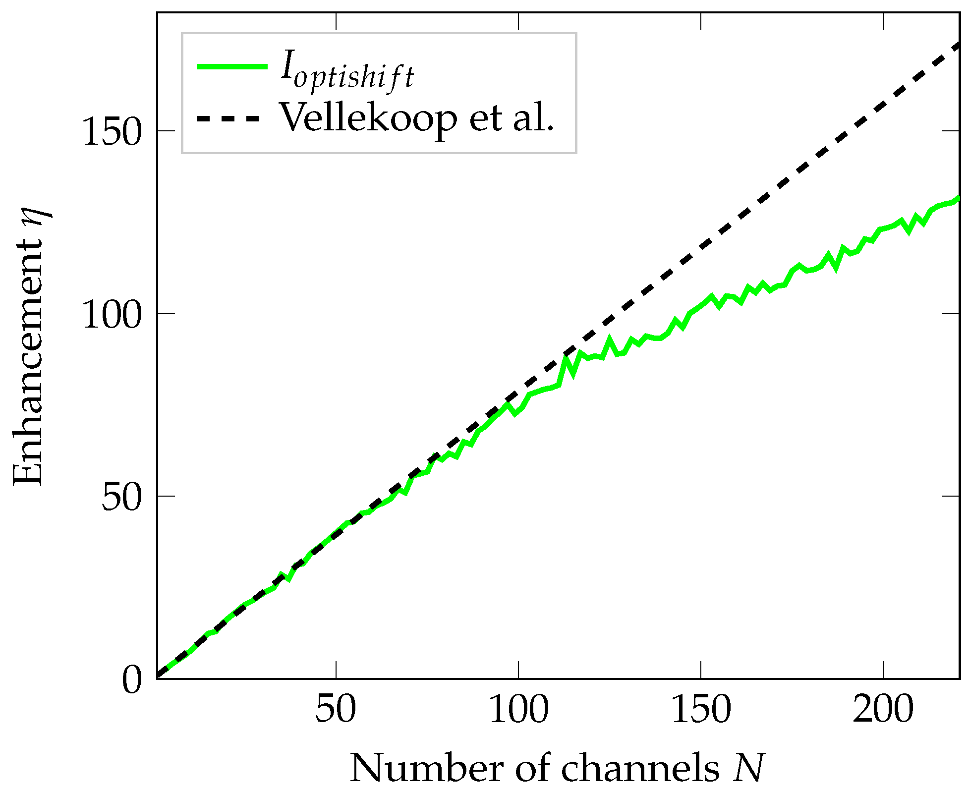
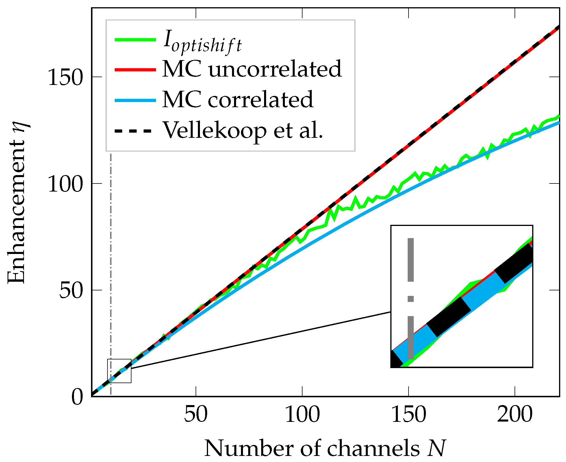
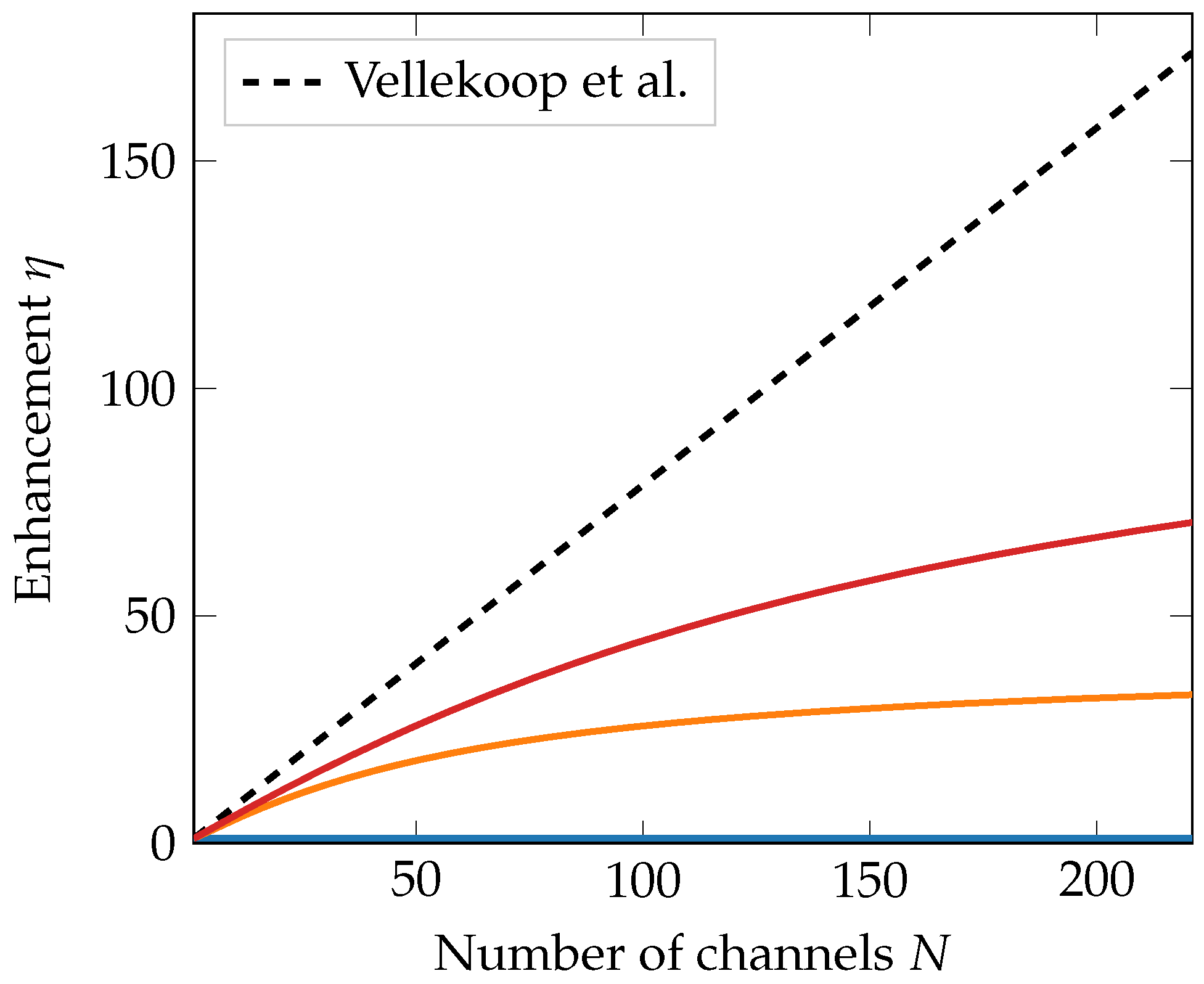
3.1. Number of Transmission Channels in a Quasi-Two-Dimensional Sample

The limit in the number of available transmission channels, already mentioned in Section 2, beyond which multiple waves (partially) couple into the same channel is considered in this section. At first, the quasi-two-dimensional problem is reduced to the consideration of a one-dimensional resonator with size L y equal to the width of the scattering medium. In the absence of sources in the linear and isotropic material, we are looking for homogeneous solutions of the wave equation. Hence, solutions of the Helmholtz equation
2 E y y 2 + k y 2 E y = 0
for the y-component of the electric field are being sought, where E y = E 0 Y ( y ) . Thus,
2 Y ( y ) y 2 + k y 2 Y ( y ) = 0
which is solved by exp ± i k y y , leading to
E y = E 0 c 1 exp ( i k y y ) + c 2 exp ( i k y y ) .
With the boundary conditions introduced by perfectly reflecting ends, implying
E y ( y = 0 ) = E y ( y = L y ) = 0
we obtain
E y = E 0 sin j π y L y .
With k y 2 = n 2 ω 2 / c 2 ( ω is the circular frequency, c the speed of light and n the refractive index) and Equations (13) and (17) one can find the dispersion relation or mode structure of the resonator
j π L y = n ω c ,
where j 1 , 2 , 3 , . Hence, the resonator only supports discrete frequencies. Rewriting Equation (18) leads to
j = ω L y n π c .
Considering a specific mode defined by a characteristic frequency ω , we now have to count the number of modes N with smaller frequencies. Rewriting Equation (19), we find the number of possible modes N to be
N = 2 n e L y λ ,
where it was that ω / c = 2 π / λ . A more detailed derivation can, e.g., be found in [31]. In Equation (20), n e is the effective refractive index approximated as the volumetric average over the refractive indices of the scattering cylinders and the surrounding medium. A factor of 2 has to be added to Equation (20) when considering the polarization of the simulated electric fields.
The transmission of light through a segment of a scattering medium is defined by the eigenvalues of a random matrix, referred to as the transmission matrix. These eigenvalues are linked to the segment’s independent transmission channels. A larger scattering medium can be described as a chain of such segments leading, in essence, to a multiplication of the transmission matrices and, hence, a multiplication of the eigenvalues. The longer the chain or the thicker the medium, the lesser eigenvalues survive until only those close to unity remain for a certain critical length. Beyond this critical length, the eigenvalues quickly decay to zero. Hence, the number of possible modes contributing to the transmission through a scattering medium is increasingly limited with increasing medium thickness L. A detailed mathematical description which can be found in [21] approximates this effective number of contributing transmission channels N e f f to be
N e f f = N L ,
where is the scattering mean free path length. To assure comparability with the simulation scenario in [24], we define L = L x . Finally, we obtain the following equation for the number of channels effectively contributing to the total transmission
N e f f = 2 n e L y λ L x .
In the three-dimensional case, Equation (22) has the form 2 π A n e 2 / λ 0 2 · / L x , where A is the illuminated area ( = π L y 2 ) , as can be found in the literature [32]. With the simulation parameters from [24] inserted into Equation (22), N e f f 10 was found to be a sufficiently good estimate for the simulation in Figure 4, as shown by the grey dashed line in the inset.

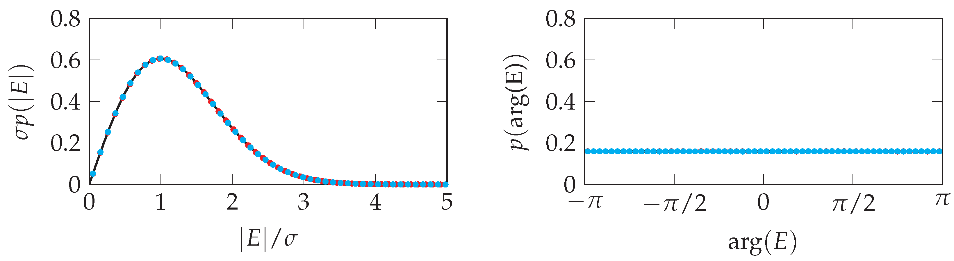
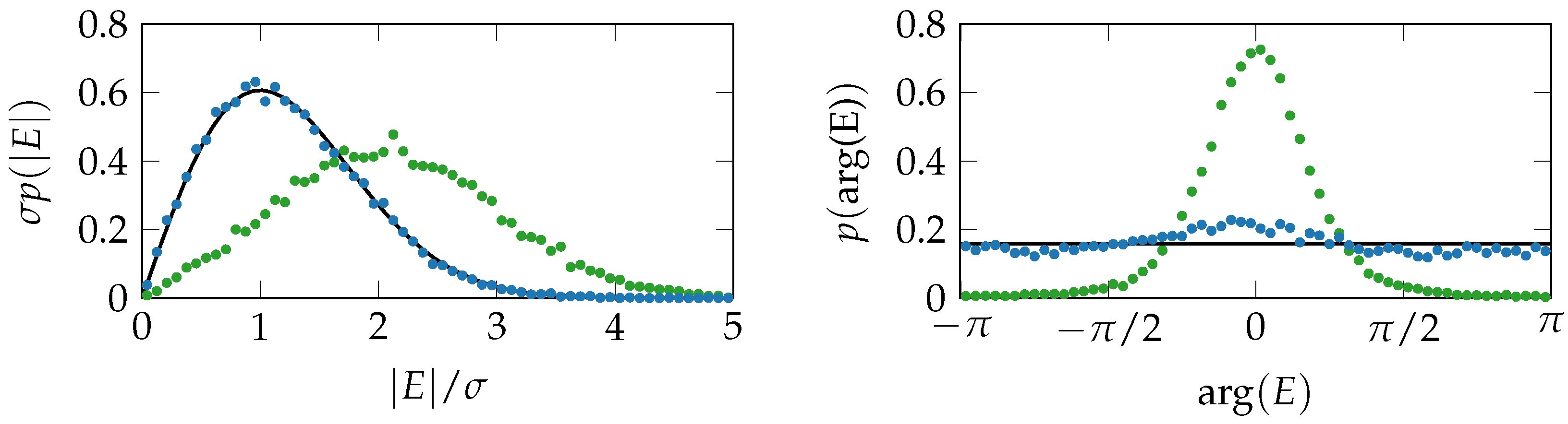
3.2. Deviations from the Circular Complex Gaussian Distribution

Non-negligible shares of ballistic and little-scattered light lead to the electric fields not being fully randomized. Therefore, they are not entirely circular complex Gaussian distributed, as already outlined in [24] for an ASPW with constant amplitude and equal phase of the incident plane waves at a location in the scattering medium close to the first surface.
This circumstance can be re-enacted by introducing a random phasor sum with a non-uniform distribution of phases; see [23]. Nevertheless, the assumption of identically distributed components remains, and the resulting distribution of the electric fields has the shape of a compressed circular complex Gaussian, which is why the amplitude remains Rayleigh distributed. The non-uniform distribution of phases was found to follow a von Mises distribution [33]. This distribution function is a close approximation to the wrapped normal distribution and confined to the interval π Θ < π . The von Mises distribution reassembles a normal distribution for small standard deviations σ and approaches the uniform distribution when σ is large. Thus, it could be used to simulate the process of the transition of a global phase of the ASPW centred around Θ = 0 before impinging on the scattering medium up to the uniform distribution after sufficient scattering.
Calculating the average normalized amplitude and phase distributions of the correlated electric fields at various depths from the data obtained in [24], WFS of electric fields that did not undergo sufficient scattering was observed as it is, e.g., the case for ballistic and little-scattered light. For this purpose, the near fields at the desired positions were superimposed according to the ASPW, as already described in Section 2.1. The lateral shift of the positions averaged at a certain depth was at least 2 λ . Figure 5 illustrates examples of the calculated distributions of the amplitude and the phase from which the electric fields were drawn. The amplitude and the phase distribution at a depth of approx. 0 λ (green) show significant deviations from the distributions expected for circular complex Gaussian distributed electric fields. Due to the rectangular function describing the amplitude of the ASPW and its global phase, a constant amplitude distribution and a peak at Θ = 0 in the phase distribution are expected. However, their shapes are altered by the influence of the field components backscattered by the medium. In blue, the amplitude and the phase distributions at a depth of approx. 20 λ are shown. A deviation from the uniform distribution of the phase is still perceptible.
Fitting a Rayleigh density function to the calculated amplitude distributions and a von Mises density function to the phase distributions delivered the necessary parameters for the MC simulation. Sampling the respective density function using these parameters and applying the correlation factors for neighbouring electric fields at each depth determined following the previously described procedure delivered the results presented in Figure 6. Due to the lack of an analytic solution for the cumulative distribution function, an algorithm proposed in [34,35] was implemented to sample the von Mises distribution function. The dataset was simulated similarly to the one shown in Figure 4, where 9216 parallelized processes averaged over 50 iterations repeatedly calculated 11,050 electric fields.
The shallower the depths from which the amplitude and the phase distributions originate, the greater the deviations from the circular complex Gaussian distribution are (see Figure 5) and, thus, the larger the deviations of the intensity enhancement from Equation (1) are, as shown in Figure 6. Changes in the amplitude and the phase distributions allow the theoretical study of WFS in areas where the light is not fully randomized in the case of uncorrelated as well as correlated electric fields.

4. Conclusions

In WFS experiments, limitations in the achievable intensity enhancement can often be observed as an effect of temperature drifts, sample instabilities, and environmental influences. When compounded by long measurement durations or dynamic processes in the sample, the speckle decorrelation time decreases significantly and limits the WFS process. After overcoming these problems, it is possible to perform experimental measurements following the theoretical curve of the intensity enhancement [1] as long as the limit of accessible open transmission channels is not reached.
Coupling in more waves into the scattering medium than independent transmission modes available further introduces an additional limit. In this publication, it was shown that correlations of neighbouring fields strongly influence the achievable intensity enhancement, even when the field distribution remains circular complex Gaussian. The introduced MC simulations confirmed the results obtained from simulations solving Maxwell’s equations without suffering from discretization and noise. This was conducted by utilizing a significantly higher number of simulated electric fields and a subsequently adjusted correlation of nearest neighbours to account for the higher sampling of the incident ASPW and the fixed NA.
For this purpose, the simulation methodology was extended to a more general consideration of correlations of neighbouring electric fields utilizing a Cholesky decomposition. Decomposing the covariance matrix of a bivariate case resulted in a lower triangular matrix that was used to generate correlated, normally distributed real and imaginary parts from previously uncorrelated ones. Knowledge of the correlation coefficient for the medium under investigation, based on its wavelength-dependent properties, is essential and can, e.g., be retrieved from further Maxwell simulations. Taking correlations between next-but-one and further neighbours into account is expected to result in even better agreement between simulations solving Maxwell’s equations and the results obtained from MC simulations. Increasing the sampling density of the NA causes a broadening of the autocorrelation peak. Therefore, the angular correlation of the electric fields increases, resulting in a larger range, where the transmitted field distribution remains sufficiently self-similar concerning angular changes in the wavefront incident on a scattering medium. Correlations in the electric fields can thus, e.g., be used to image a region inside or behind a scattering medium enlarged due to the growing angular invariance without changes to the incident field. This phenomenon is known as the angular memory effect mentioned in the introduction. For further details, see [17,18,19,20].
An estimate of the limit of independent open transmission channels in quasi-two dimensions was presented, and thus, a method to set meaningful parameters for experiments considering this threshold value. With that, the expected value of independent open transmission channels and the influence of correlations of neighbouring electric fields on WFS can be determined before experiments.
The presented MC simulation further allowed studying scenarios where the prerequisite for optimal WFS, namely a circular complex Gaussian distribution of (uncorrelated) electric fields, was not given due to, e.g., the influence of ballistic and little-scattered light. Thus, the methodology presented allows theoretical investigations of WFS beyond ideal conditions and to utilize the knowledge gained in future measurements. Experiments on WFS in general and especially under the influence of ballistic light on volume-scattering phantoms have already been performed by us [36] and can be extended to the limit of correlated transmission modes.
Overall, the methodology presented contributes to a better understanding of the correlations of electric fields deep inside scattering media and delivers a promising approach to the existing limitations of, e.g., the application of correlation-based imaging.
Experimental validation of the results obtained can be achieved by measurements on precisely fabricated samples. For example, a nano printer is an excellent choice for printing a suitable cylinder distribution as used in the simulations solving Maxwell’s equations. Knowing the effective refractive index determined by the chosen photoresist and the concentration of scatterers, together with the diameter of the illumination spot on the sample and its thickness, all that remains is to calculate the respective scattering mean free path length. It can be, e.g., determined with the analytical solution of Maxwell’s equations under the assumption of independent scattering. Optimizing the incident ASPW experimentally could be conducted with a spatial light modulator (SLM), where the pixels of the SLM allow clustering of the waves impinging the sample.
Further investigations into the influence of absorption as a limiting factor of WFS are of great interest as well. Particularly at low depths, the total radiance is dominated by ballistic and little-scattered light. Absorption expands this circumstance further into the medium, thus decreasing the capability of WFS in this area and consequently lowering the achievable intensity enhancement.
With the method and results presented in this paper, it is possible to perform extensive theoretical investigations of WFS, which can be compared to measurements on fabricated and well-characterized scattering samples with specific optical and geometrical properties regarding the desired correlations of electric fields, taking the parameters in Equation (22) into account.

Author Contributions

Conceptualization, N.F., F.O., D.R. and A.K.; methodology, N.F., F.O. and D.R.; software, N.F. and D.H.; formal analysis, N.F., F.O. and A.K.; investigation, N.F.; resources, A.K.; writing—original draft preparation, N.F.; writing—review and editing, N.F., F.O., D.R. and A.K.; visualization, N.F.; supervision, A.K.; project administration, A.K.; funding acquisition, A.K. All authors have read and agreed to the published version of the manuscript.

Funding

This work was supported by the the Deutsche Forschungsgemeinschaft (DFG, German Research Foundation) under project number 322575.

Institutional Review Board Statement

Not applicable.

Informed Consent Statement

Not applicable.

Data Availability Statement

Data underlying the results presented in this paper are not publicly available at this time but may be obtained from the authors upon reasonable request.

Conflicts of Interest

The authors declare no conflicts of interest.

References

  1. Vellekoop, I.M.; Mosk, A.P. Focusing coherent light through opaque strongly scattering media. Opt. Lett. 2007, 32, 2309–2311. [Google Scholar] [CrossRef] [PubMed]
  2. Vellekoop, I.M.; Lagendijk, A.; Mosk, A. Exploiting disorder for perfect focusing. Nat. Photonics 2010, 4, 320–322. [Google Scholar] [CrossRef]
  3. Vellekoop, I.M. Feedback-based wavefront shaping. Opt. Express 2015, 23, 12189–12206. [Google Scholar] [CrossRef]
  4. Gigan, S.; Katz, O.; de Aguiar, H.B.; Andresen, E.R.; Aubry, A.; Bertolotti, J.; Bossy, E.; Bouchet, D.; Brake, J.; Brasselet, S.; et al. Roadmap on wavefront shaping and deep imaging in complex media. J. Phys. Photonics 2022, 4, 042501. [Google Scholar] [CrossRef]
  5. Devaud, L.; Rauer, B.; Mauras, S.; Rotter, S.; Gigan, S. Correlating light fields through disordered media across multiple degrees of freedom. arXiv 2023, arXiv:2312.08506. [Google Scholar]
  6. Song, L.; Zhou, Z.; Wang, X.; Zhao, X.; Elson, D.S. Simulation of speckle patterns with predefined correlation distributions. Biomed. Opt. Express 2016, 7, 798–809. [Google Scholar] [CrossRef] [PubMed]
  7. Kim, M.; Choi, Y.; Yoon, C.; Choi, W.; Kim, J.; Park, Q. Maximal energy transport through disordered media with the implementation of transmission eigenchannels. Nat. Photonics 2012, 6, 581–585. [Google Scholar] [CrossRef]
  8. Verrier, N.; Depraeter, L.; Felbacq, D.; Gross, M. Measuring enhanced optical correlations induced by transmission open channels in a slab geometry. Phys. Rev. B 2016, 93, 161114. [Google Scholar] [CrossRef]
  9. Sarma, R.; Yamilov, A.G.; Petrenko, S.; Bromberg, Y.; Cao, H. Control of Energy Density inside a Disordered Medium by Coupling to Open or Closed Channels. Phys. Rev. Lett. 2016, 117, 086803. [Google Scholar] [CrossRef]
  10. Yilmaz, H.; Hsu, C.W.; Yamilov, A.; Cao, H. Transverse localization of transmission eigenchannels. Nat. Photonics 2019, 13, 352–358. [Google Scholar] [CrossRef]
  11. Bender, N.; Yamilov, A.; Yilmaz, H.; Cao, H. Fluctuations and Correlations of Transmission Eigenchannels in Diffusive Media. Phys. Rev. Lett. 2020, 125, 165901. [Google Scholar] [CrossRef] [PubMed]
  12. Venderbosch, P.; van der Meer, R.; de Goede, M.; Kassenberg, B.; Snijders, H.; Epping, J.; Taballione, C.; van den Vlekkert, H.; Renema, J.J.; Pinkse, P.W.H. Observation of Open Scattering Channels. In Proceedings of the Integrated Photonics Research, Silicon and Nanophotonics, Maastricht, The Netherlands, 24–28 July 2022; Optica Publishing Group: Washington, DC, USA, 2022. [Google Scholar]
  13. Cao, H.; Mosk, A.P.; Rotter, S. Shaping the propagation of light in complex media. Nat. Phys. 2022, 18, 994–1007. [Google Scholar] [CrossRef]
  14. Pai, P.; Bosch, J.; Kühmayer, M.; Rotter, S.; Mosk, A.P. Scattering invariant modes of light in complex media. Opt. Express 2015, 23, 12189–12206. [Google Scholar] [CrossRef]
  15. Katz, O.; Small, E.; Silberberg, Y. Looking around corners and through thin turbid layers in real time with scattered incoherent light. Nat. Photonics 2012, 6, 549–553. [Google Scholar] [CrossRef]
  16. Jauregui-Sánchez, Y.; Penketh, H.; Bertolotti, J. Tracking moving objects through scattering media via speckle correlations. Nat. Commun. 2022, 13, 5779. [Google Scholar] [CrossRef]
  17. Judkewitz, B.; Horstmeyer, R.; Vellekoop, I.M.; Papadopoulos, I.N.; Yang, C. Translation correlations in anisotropically scattering media. Nat. Phys. 2015, 11, 684–689. [Google Scholar] [CrossRef]
  18. Schott, S.; Bertolotti, J.; Léger, J.F.; Bourdieu, L.; Gigan, S. Characterization of the angular memory effect of scattered light in biological tissues. Opt. Express 2015, 23, 13505–13516. [Google Scholar] [CrossRef]
  19. Osnabrugge, G.; Horstmeyer, R.; Papadopoulos, I.N.; Judkewitz, B.; Vellekoop, I.M. Generalized optical memory effect. Optica 2017, 4, 886–892. [Google Scholar] [CrossRef]
  20. Yilmaz, H.; Hsu, C.W.; Goetschy, A.; Bittner, S.; Rotter, S.; Yamilov, A.; Cao, H. Angular Memory Effect of Transmission Eigenchannels. Phys. Rev. Lett. 2019, 123, 203901. [Google Scholar] [CrossRef] [PubMed]
  21. Imry, Y. Active Transmission Channels and Universal Conductance Fluctuations. Europhys. Lett. 1986, 1, 249. [Google Scholar] [CrossRef]
  22. Goodman, J.W. Statistical Optics, 2nd ed.; Wiley-Interscience: New York, NY, USA, 2015. [Google Scholar]
  23. Goodman, J.W. Speckle Phenomena in Optics: Theory and Applications, 2nd ed.; SPIE: Bellingham, WA, USA, 2020. [Google Scholar]
  24. Ott, F.; Fritzsche, N.; Kienle, A. Numerical simulation of phase-optimized light beams in two-dimensional scattering media. J. Opt. Soc. Am. 2022, 39, 2410–2421. [Google Scholar] [CrossRef]
  25. Bar, C.; Alterman, M.; Gkioulekas, I.; Levin, A. Monte-Carlo simulation of the memory effect in random media beyond the diffusion limit. In Proceedings of the Optical Coherence Imaging Techniques and Imaging in Scattering Media III, Munich, Germany, 23–27 June 2019; Volume EB105 of SPIE Proceedings. Optica Publishing Group: Washington, DC, USA, 2019. [Google Scholar]
  26. Bewick, J.A.J.; Munro, P.R.T.; Arridge, S.R.; Guggenheim, J.A. Scalable full-wave simulation of coherent light propagation through biological tissue. In Proceedings of the 2021 IEEE Photonics Conference (IPC), Vancouver, BC, Canada, 18–21 October 2021; pp. 1–2. [Google Scholar]
  27. Neves, S.; Araujo, F. Fast and Small Nonlinear Pseudorandom Number Generators for Computer Simulation. In Parallel Processing and Applied Mathematics; Wyrzykowski, R., Dongarra, J., Karczewski, K., Waśniewski, J., Eds.; Springer: Berlin/Heidelberg, Germany, 2012; pp. 92–101. [Google Scholar]
  28. Ciglarič, T.; Češnovar, R.; Štrumbelj, E. An OpenCL library for parallel random number generators. J. Supercomput. 2019, 75, 3866–3881. [Google Scholar] [CrossRef]
  29. Gilli, M.; Maringer, D.; Schumann, E. Numerical Methods and Optimization in Finance, 1st ed.; Academic Press: Cambridge, MA, USA, 2011. [Google Scholar]
  30. Dainty, J.C. The Statistics of Speckle Patterns; Elsevier: Amsterdam, The Netherlands, 1977; Volume 14, pp. 1–46. [Google Scholar]
  31. Griffiths, D.J. Introduction to Electrodynamics, 5th ed.; Cambridge University Press: Cambridge, UK, 2023. [Google Scholar]
  32. Ojambati, O.S.; Hosmer-Quint, J.T.; Gorter, K.-J.; Mosk, A.P.; Vos, W.L. Controlling the intensity of light in large areas at the interfaces of a scattering medium. Phys. Rev. A 2016, 94, 043834. [Google Scholar] [CrossRef]
  33. Von Mises, R. Über die ’Ganzzahligkeit’ der Atomgewichte und verwandte Fragen. Phys. Z. 1918, 19, 490–500. [Google Scholar]
  34. Best, D.J.; Fisher, N.I. Efficient Simulation of the von Mises Distribution. J. Appl. Stat. 1979, 28, 152–157. [Google Scholar] [CrossRef]
  35. Fisher, N.I. Statistical Analysis of Circular Data; Cambridge University Press: Cambridge, UK, 1993. [Google Scholar]
  36. Fritzsche, N.; Ott, F.; Pink, K.; Kienle, A. Focusing Coherent Light through Volume Scattering Phantoms via Wavefront Shaping. Sensors 2023, 23, 8397. [Google Scholar] [CrossRef] [PubMed]
Figure 1. Intensity enhancement η over the number of channels N resulting from simulations solving Maxwell’s equations. The black dashed line shows the theoretically expected value according to Equation (1) following [1]. I o p t i s h i f t data taken from [24].
Photonics 11 00797 g001
Figure 2. Average autocorrelation of the uncorrelated (red, ρ = 0 ) and correlated (blue, ρ = 0.118 ) electric fields over the k-vector spacing at N = 221 .
Photonics 11 00797 g002
Figure 3. Normalized, average distribution of the amplitude (left) and the phase (right) of the electric fields. Depicted in red is the uncorrelated ( ρ = 0 ) case, and in light blue is the correlated case ( ρ = 0.928 ). The black solid lines show the theoretical density functions (left: Equation (4), right: Equation (5)).
Photonics 11 00797 g003
Figure 4. Comparison of the intensity enhancement η over the number of channels N obtained by solving Maxwell’s equations (orange) and the Monte Carlo (MC) simulation. The correlation coefficient in the uncorrelated case (red) is given with ρ = 0 . For the correlated fields (light blue) ρ = 0.928 . The black dashed line shows the theoretically expected value according to Equation (1) following [1]. Indicated by the vertically dashed grey line at N = 10 , the point is marked, where the intensity enhancements of the correlated and uncorrelated electric fields approximately start to deviate.
Photonics 11 00797 g004
Figure 5. Normalized average distribution of the amplitude (left) and the phase (right) of the correlated electric fields at a depth of approx. 0 λ (green) and approx. 20 λ (blue). The black solid lines show the theoretical density functions of the amplitude and the phase for circular complex Gaussian-distributed electric fields.
Photonics 11 00797 g005
Figure 6. MC simulation of the intensity enhancement η over the number of channels N for not completely circular complex Gaussian distributed electric fields. Depicted are the intensity enhancement for depths of approx. 20 λ (blue), approx. 40 λ (orange), and approx. 80 λ (red). All electric fields were calculated with their respective adapted correlation factor. The black dashed line shows the theoretically expected value according to Equation (1) following [1].
Photonics 11 00797 g006
Disclaimer/Publisher’s Note: The statements, opinions and data contained in all publications are solely those of the individual author(s) and contributor(s) and not of MDPI and/or the editor(s). MDPI and/or the editor(s) disclaim responsibility for any injury to people or property resulting from any ideas, methods, instructions or products referred to in the content.

