Interferometrically Enhanced Intensity and Wavelength Modulation in Tunable Diode Laser Spectroscopy

Abstract

Tunable diode laser spectroscopy (TDLS) is a measurement technique with high spectral resolution. It is based on tuning the emission wavelength of a semiconductor laser by altering its current and/or its temperature. However, adjusting the wavelength leads to a change in emission intensity. For applications that rely on modulated radiation, the challenge is to isolate the true spectrum from the influence of extraneous instrumental contributions, particularly residual intensity and wavelength modulation. We present a novel approach combining TDLS with interferometric techniques, exemplified by the use of a Mach–Zehnder interferometer, to enable the separation of intensity and wavelength modulation. With interferometrically enhanced intensity modulation, we reduced the residual wavelength modulation by 83%, and with interferometrically enhanced wavelength modulation, we almost completely removed the residual derivative of the signal. A reduction in residual wavelength modulation enhances the spectral resolution of intensity-modulated measurements, whereas a reduction in residual intensity modulation improves the signal-to-noise ratio and the sensitivity of wavelength-modulated measurements.

1. Introduction

The radiation intensity and emission wavelength of a semiconductor laser change as a function of the laser current. With its narrow emission bandwidth, this tunable monochromatic light source is well suited for spectroscopic applications, which are widely known as tunable diode laser spectroscopy (TDLS) [1].

In comparison to a continuous change in laser current, the use of a modulated current offers the advantage of greatly improved signal-to-noise ratio through the phase-sensitive detection of the emitted radiation. This can be accomplished with a lock-in amplifier, which allows for the recognition of even the smallest features of the spectrum [2].

A number of methods may be used to modulate laser radiation. Mechanical modulators are straightforward to implement and are suitable for use in the UV, VIS, and the entire IR range. However, they are typically less frequency-stable compared to electro-optical modulation [3]. Electro-optical modulators are frequency-stable across a broad range of frequencies, which is a key factor in their widespread use in telecommunications [4]. One limitation of these devices in free-space IR spectroscopy applications is that the required operating voltage increases proportionally to the wavelength of the light to be modulated. Recent advancements in integrated photonics have enabled the use of smaller voltages due to the miniaturization of the underlying structures [5]. The direct modulation of the laser current is a particularly simple method that is frequency-stable and applicable across the entire operating wavelength range of the laser. However, the relation between emitted radiation intensity and wavelength is challenging for spectroscopic measurements [6].

In TDLS, the light modulation of a semiconductor laser is performed by modulating its injection current, which results in a combined intensity modulation (IM) and wavelength modulation (WM) with a phase relation between the two. The phase shift between IM and WM varies depending on the laser, but typically decreases from lower to higher modulation frequencies [7]. Therefore, it is quite chalenging to compensate the respective undesired effect.

In wavelength modulation spectroscopy (WMS), researchers are interested in the signals generated solely by the WM of the laser emission. IM distorts the spectrum and is therefore referred to as residual amplitude modulation [7]. Derivative spectroscopy offers the advantage of isolating changes in the sample’s transmissivity with wavelength, removing the background signal from transmitted or reflected light. This improves the resolution of weak and overlapping spectral features compared to direct absorption or reflection spectroscopy [8,9].

The main challenge in WMS is eliminating spectral distortion caused by the wavelength dependences of emission intensity $I_{\mathrm{e}}$, detector responsivity G, and steering optics. In a basic absorption experiment with non-dispersive optics, the detector signal $S=I_{\mathrm{e}}GT$, where T is the sample transmissivity. The normalized derivative signal is

$${\displaystyle \frac{1}{S}}{\displaystyle \frac{\mathrm{d}S}{\mathrm{d}\lambda }}\Delta \lambda =\left({\displaystyle \frac{1}{I_{\mathrm{e}}}}{\displaystyle \frac{\mathrm{d}{I}_{\mathrm{e}}}{\mathrm{d}\lambda }}+{\displaystyle \frac{1}{G}}{\displaystyle \frac{\mathrm{d}G}{\mathrm{d}\lambda }}\right)\Delta \lambda +{\displaystyle \frac{1}{T}}{\displaystyle \frac{\mathrm{d}T}{\mathrm{d}\lambda }}\Delta \lambda .$$

(1)

where $\Delta \lambda$ is the depth of the wavelength modulation [8].

Common solutions to address unwanted contribution from wavelength dependences in intensity and detector responsivity are dual-beam single-detector spectrophotometers with alternate sampling [6,10] and dual-beam double-detector spectrophotometers with simultaneous sampling [8].

In the following sections, we will present an alternative method that combines TDLS with an interferometer and offers a particularly easy reduction in the respective undesired effect. In Section 2, we present the materials and methods used to achieve interferometrically enhanced modulation. Section 3 contains the experimental and computational results which will subsequently be discussed in Section 4.

2. Materials and Methods

In this section, we present the materials and methods used to achieve interferometrically enhanced modulation. This includes the basics of the Mach–Zehnder interferometer (MZI), the characteristics of the used interband cascade laser (ICL), as well as the experimental setup, followed by the computational theory.

2.1. Mach–Zehnder Interferometer

A basic Mach–Zehnder interferometer with balanced path lengths is shown in Figure 1. It consists of a pair of beam splitters (BS₁, BS₂) and a pair of mirrors (M_a, M_b), one in each of the optical paths. At the first beam splitter BS₁, the incoming laser light $I_{\mathrm{e}}$ is split and travels along two distinct paths, labelled as a and b. The light is then recombined at the second beam splitter BS₂, resulting in two outputs $I_{\mathrm{MZI}}$ and $I_{\mathrm{MZI}}^{\prime }$. The interference pattern observed at the output is highly sensitive to phase differences that result from path length differences.

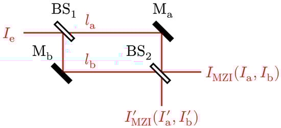
Figure 1. Balanced Mach–Zehnder interferometer.

The use of an interferometer, in our case an MZI, enhances modulation in two ways:

• It allows IM at reduced residual wavelength modulation through the use of alternating destructive and constructive interferences;
• It allows WM with almost constant intensity by modulating on stationary points of the interference signal.

The benefit of using an MZI over other interferometers is that we can completely avoid back reflection to protect the semiconductor laser. Alternatives to the MZI are Michelson or Fabry–Pérot interferometers.

2.2. Interband Cascade Laser

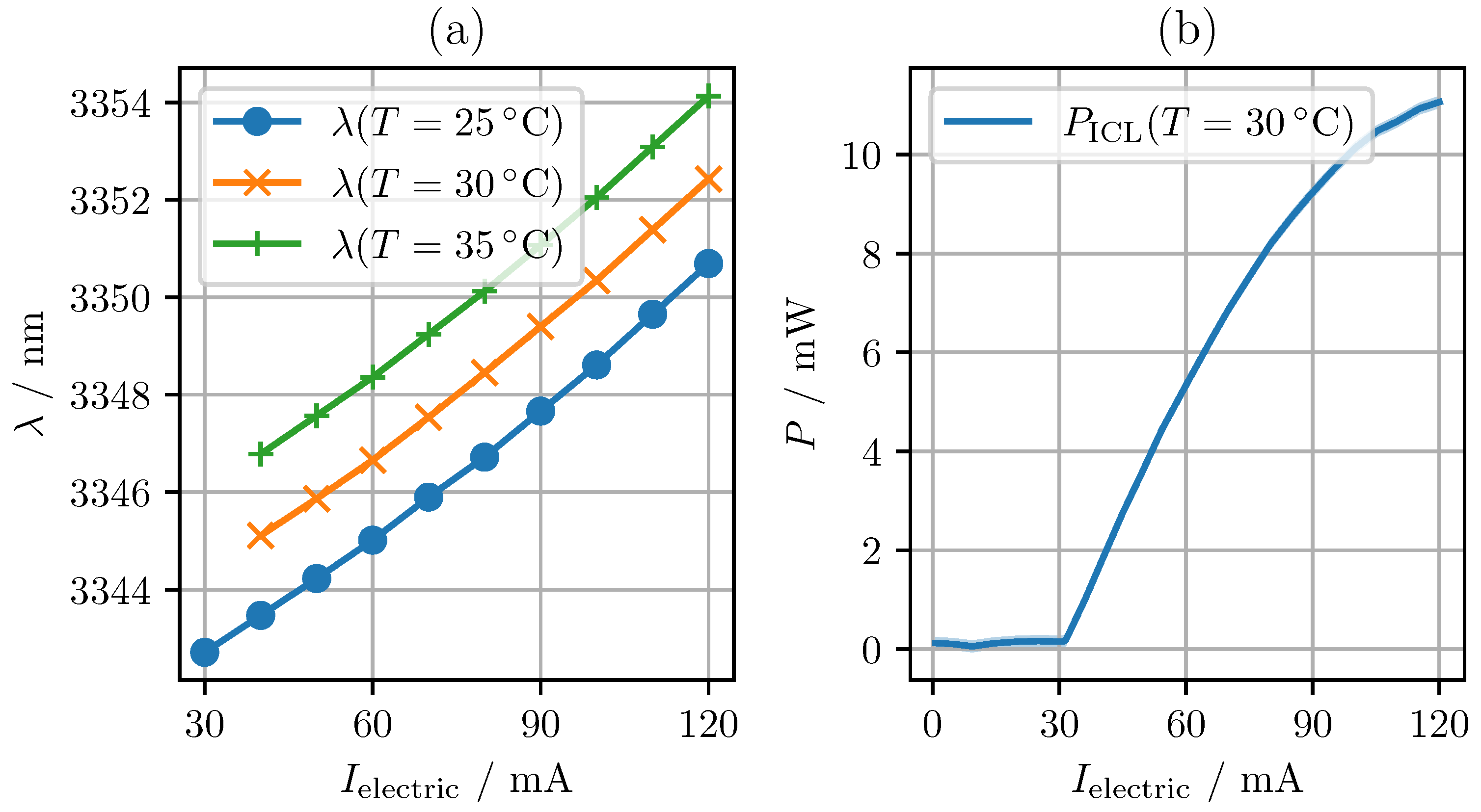
In order to characterize the wavelength behavior of the laser in relation to its current and temperature, we use the data provided by the manufacturer, Nanoplus (Meiningen, Germany). Figure 2a illustrates the current–wavelength dependency at three distinct temperatures. Through linear regression, we obtain a wavelength-to-current slope of (0.0907 ± 0.0020) nm/mA and a wavelength-to-temperature slope of (0.3386 ± 0.0032) nm/°C. The uncertainties represent the standard deviations according to Appendix A.1 Equation (A3). Figure 2b illustrates the relationship between laser current and optical power. The threshold current of the laser is 30 mA and the emission power–current slope equals 0.181 mW/mA assuming linear regression. This allows output powers of up to 11 mW and exhibits a beam width of (2.42 ± 0.12) mm (90% fit).

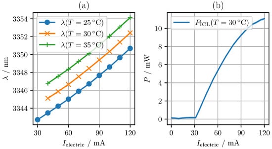
Figure 2. (a) Wavelength $\lambda$ of ICL for currents $I_{\mathrm{electric}}$ from 30 mA to 120 mA at three different temperatures. (b) Optical power P of ICL for currents $I_{\mathrm{electric}}$ up to 120 mA. The data were provided by Nanoplus (Meiningen, Germany).

A key parameter of the laser is its spectral linewidth γ, which directly impacts the coherence length $l_{\mathrm{coherence}}$ of the emitted radiation [11,12]

$$l_{\mathrm{coherence}}={\displaystyle \frac{{\lambda }_{\mathrm{center}}^2}{{\lambda }_{\mathrm{FWHM}}}}.$$

(2)

For a center wavelength ${\lambda }_{\mathrm{center}}$ of 3350 nm and $\gamma$ of 3 MHz, or ${\lambda }_{\mathrm{FWHM}}=$ 0.11 pm, this results in a coherence length of $l_{\mathrm{coherence}}=$ 30 m.

2.3. Experimental Setup

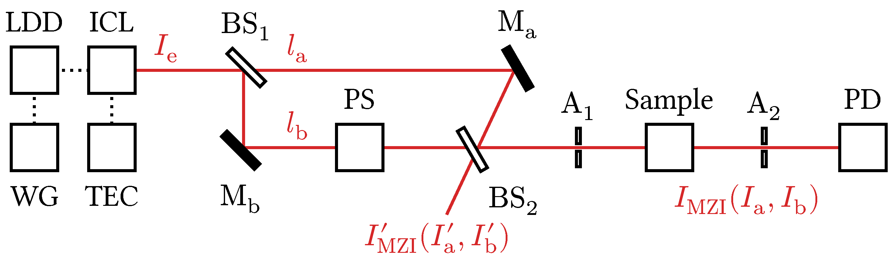
Figure 3 shows the experimental setup for interferometrically enhanced (IE) modulation in TDLS. All relevant components and their parameters are listed in Appendix A Table A1. As radiation source serves the above described distributed feedback (DFB) ICL with a center wavelength of 3349.7 nm. The laser diode driver (LDD) is controlling the operation current, while the thermoelectric cooler (TEC) controller maintains a constant temperature. A waveform generator (WG) provides the laser current setpoint to the driver.

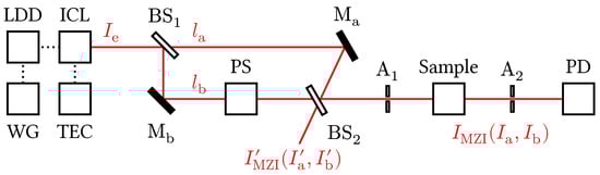
Figure 3. Experimental setup for interferometrically enhanced modulation.

The MZI is a free beam design that allows for adjustable path length $l_{\mathrm{a}}$ and $l_{\mathrm{b}}$. The beam splitters BS₁ and BS₂ are 5 mm thick CaF₂ plates with a coating optimized for wavelengths between 2 and 8 μm. The radiation reflected by the beam splitters, as well as by the protected silver mirrors M_a and M_a experiences a 180° phase shift, while the passing radiation remains unaltered. Radiation passing through a beam splitter experiences a longer optical path which is a consequence of the higher optical density of CaF₂ compared to air. Since beam a passes BS₁ and beam b passes BS₂, the individual paths are roughly equal.

The distance between the ICL and the detector passing through path b is 149 cm.

The two iris diaphragms A₁ and A₂ (alternatively, pinhole apertures can be used) allow the precise alignment of the interfering beams. The gas sample is positioned between A₁ and A₂ in a vacuum-sealed 30 cm long cell with 3 mm thick CaF₂ windows.

To detect the MZI’s transmission, an Indium Arsenide Antimonide (InAsSb) fixed-gain amplified photodetector (PD), sensitive for wavelengths from 2.7 μm to 5.3 μm, with a transimpedance gain at Hi-Z of 300 kV A⁻¹, is utilised. The active area of the detector has a size of 0.7 mm × 0.7 mm, which is smaller than the beam width of 2.42 mm. The sensor’s responsivity at a temperature of 19 °C and a wavelength of 3.35 μm is (4.7 ± 0.2) mA W⁻¹. This results in an amplification of (1.41 ± 0.06) V mW⁻¹ at the detector output. A 14 bit, 250 kS/s data acquisition card converts the analogue detector signal into a digital one, which is then stored and evaluated.

The length of $l_{\mathrm{b}}$ from BS₁ to BS₂ is 35 cm, whereas BS₁ and M_b reflect the beam exactly at a 45° angle. The length of $l_{\mathrm{a}}$ from BS₁ to BS₂ is 36 cm. This distance is slightly longer due to smaller reflection angles of 40°. The ICL and the detector are 149 and 150 cm, respectively. The different concepts for phase shifter (PS) are described in Section 2.6.

2.4. Interference Model

To describe the output intensity $I_{\mathrm{MZI}}$ of the MZI, we begin with the general equation for the interference of two beams, labeled a and b [13].

$$I_{\mathrm{MZI}}=I_{\mathrm{a}}+I_{\mathrm{b}}+2\sqrt{I_{\mathrm{a}}{I}_{\mathrm{b}}}cos({\phi }_{\mathrm{a}}-{\phi }_{\mathrm{b}}),$$

(3)

with the intensities $I_{\mathrm{a}}$, $I_{\mathrm{b}}$ and their phases ${\phi }_{\mathrm{a}}$, ${\phi }_{\mathrm{b}}$. The phase of each beam is determined by the wavelength $\lambda$ and the path lengths $l_{\mathrm{a}}$, $l_{\mathrm{b}}$ and the average refractive index n

$$\begin{array}{cc}\hfill {\phi }_{\mathrm{a}}& ={\displaystyle \frac{2\pi l_{\mathrm{a}}n}{\lambda }},\hfill \end{array}$$

(4)

$$\begin{array}{cc}\hfill {\phi }_{\mathrm{b}}& ={\displaystyle \frac{2\pi l_{\mathrm{b}}n}{\lambda }}.\hfill \end{array}$$

(5)

The difference between ${\phi }_{\mathrm{a}}$ and ${\phi }_{\mathrm{b}}$ can be expressed as

$${\phi }_{\mathrm{MZI}}={\displaystyle \frac{2\pi dn}{\lambda }},$$

(6)

with the difference of the path lengths $d=l_{\mathrm{a}}-l_{\mathrm{b}}$.

From Equation (6), we can see that the wavelength affects the phase. We want to exploit this circumstance and generate a path difference that leads to a wavelength-dependent phase change $\Delta {\phi }_{\mathrm{MZI},\lambda }$

$$\begin{array}{cc}\hfill \Delta {\phi }_{\mathrm{MZI},\lambda }& ={\phi }_{\mathrm{MZI}}\left({\lambda }_1\right)-{\phi }_{\mathrm{MZI}}\left({\lambda }_0\right),\hfill \end{array}$$

(7)

$$\begin{array}{cc}\hfill & ={\displaystyle \frac{2\pi dn}{{\lambda }_1}}-{\displaystyle \frac{2\pi dn}{{\lambda }_0}},\hfill \end{array}$$

(8)

$$\begin{array}{cc}\hfill & ={\displaystyle \frac{2\pi dn{\lambda }_0}{{\lambda }_1{\lambda }_0}}-{\displaystyle \frac{2\pi dn{\lambda }_1}{{\lambda }_0{\lambda }_1}},\hfill \end{array}$$

(9)

$$\begin{array}{cc}\hfill & =2\pi dn{\displaystyle \frac{{\lambda }_1-{\lambda }_0}{{\lambda }_0{\lambda }_1}}.\hfill \end{array}$$

(10)

2.5. Modulation Efficiency

Equation (3) is the exact solution for the intensity of an ideal interferometer. It should be noted that several technical factors may influence the observable intensities ${\widehat{I}}_{\mathrm{MZI}}$, ${\widehat{I}}_{\mathrm{a}}$, and ${\widehat{I}}_{\mathrm{b}}$. In what follows, experimental values are always notated with a hat, as in ${\widehat{I}}_{\mathrm{a}}$. In order to make Equation (3) applicable to our setup, we introduce the interference efficiency factor ${\eta }_{\mathrm{MZI}}$, to obtain

$${\widehat{I}}_{\mathrm{MZI}}={\widehat{I}}_{\mathrm{a}}+{\widehat{I}}_{\mathrm{b}}+2\sqrt{{\widehat{I}}_{\mathrm{a}}{\widehat{I}}_{\mathrm{b}}}cos\left({\phi }_{\mathrm{MZI}}\right){\eta }_{\mathrm{MZI}}.$$

(11)

The observable intensity may be influenced by an interference pattern on the photodetector, which can be caused by the beam divergence of the laser or the misalignment of the two beams [11]. A schematic interference pattern, which is commonly associated with divergent beams, can be seen in Figure 4a. However, a detector with a small sensitive area like ours will not measure the outer interference pattern, but only the interference of the beam center. Furthermore, the intensity of a Gaussian beam decreases with increasing distance from its center, thereby reducing the influence of the outer interference patterns. An additional effect from misalignment can be an incomplete overlap of the two beam profiles, leaving the non-overlapping parts unaffected from interference, as shown in Figure 4b. As both the beam in path a and the beam in path b are reflected identically, the spatial intensity profiles of the beams have a high degree of overlap.

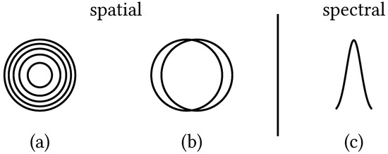
Figure 4. Influences on the interference efficiency factor include (a) beam divergence, (b) beam misalignment, and (c) the source emission spectrum.

In addition to the spatial effects, there is also a potential influence of the laser’s spectral linewidth on the wavelength dependent interference, illustrated in Figure 4c. As the linewidth of the ICL is narrow, below 3 MHz, this effect is not observed in our measurements.

It is essential to minimize the spatial influences on ${\eta }_{\mathrm{MZI}}$ by ensuring the proper alignment and collimation of the beam and validate the maximal allowed path length difference, constrained by the coherence length [11,12]. The path length difference d is considerably smaller than the coherence length of the laser $d\ll l_{\mathrm{coherence}}$ (see Section 2.2 Equation (2)), which is why this should not have a significant impact on the interference.

2.6. Tunable Phase Shift

A tunable phase shifter is essential for compensating phase drift resulting from temperature changes and for shifting the modulation point. The modulation point is the point at which the $I_{\mathrm{mzi}}$ change is minimal for wavelength modulation and maximal for intensity modulation.

A tunable phase shift can be achieved in a number of ways:

• Through an electro-optical phase shifter, typically a lithium niobate or lithium tantalate crystal, employed in one of the interferometer arms. It is actuated by voltages up to 1.7 kV for the 3 μm wavelength region [14].
• Through a linear piezo-actuated mirror positioned at either M_a or M_b; see Figure 3. The optical path length is altered by the transversal motion of the mirror, which in turn results in a phase change.
• Through a tilting window placed in one of the interferometer arms and actuated by a piezoelectric crystal or a stepper motor, thereby modifying the optical path length through internal refraction; see Figure 5. The parallel shift introduced by the window may be compensated for by the introduction of a second counter-rotating window.
  

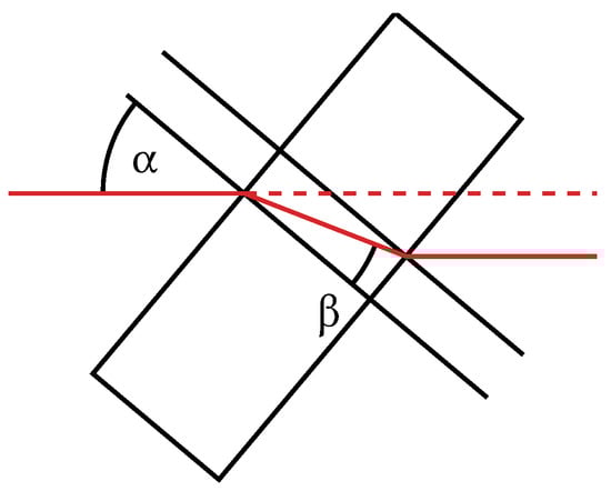  Figure 5. Tilted window with the angle of incidence $\alpha$ and the angle of refraction $\beta$ inside the window.

For a modulated phase in the kHz range, the electro-optic phase shifter is an optimal choice, as demonstrated in [14]. For slow adjustments, the piezo mirror or tilting mirror are to be preferred, given their lower cost, larger aperture, and lack of high voltage requirements. Due to the interferometer’s sensitivity to changes in the reflective angle of the mirrors, we selected the tilting window for our application.

We utilized a 2 mm thick CaF₂ window in a kinematic mount (PS in Figure 3). The mirror mount exhibited an angular range of ±4° and a resolution of 0.5° per revolution of its adjustment screw.

To reduce reflection, the window was initially positioned at the Brewster angle of CaF₂ ${\alpha }_{\mathrm{Brewster}}$ and subsequently tilted by ±1°. The Brewster angle was calculated by [13]

$${\alpha }_{\mathrm{Brewster}}={tan}^{-1}\left({\displaystyle \frac{n_{{\mathrm{CaF}}_2}}{n_{\mathrm{air}}}}\right)=54.76°$$

using the refractive index of CaF₂ $n_{{\mathrm{CaF}}_2}=1.4152$, at 3.35 μm and 24 °C [15,16]. It was observed that a change in angle of incidence of 1° results in a transition from destructive to constructive interference, corresponding to a phase change of 180°. Further details regarding the refraction of CaF₂ can be found in Appendix A.2. The relationship between the angle of incidence and the (CaF₂ window internal) angle of refraction is shown in Figure A1.

3. Results

In this section, we present our measurements obtained with the setup described in Section 2.3. The goal was to validate the analytical equations of the IE modulation technique. The temperature of the ICL was maintained at a constant 30 °C across all measurements. The ICL current was increased linearly up to 100 mA. All uncertainties of measurement are expressed as the standard error. For more information, see Appendix A.1.

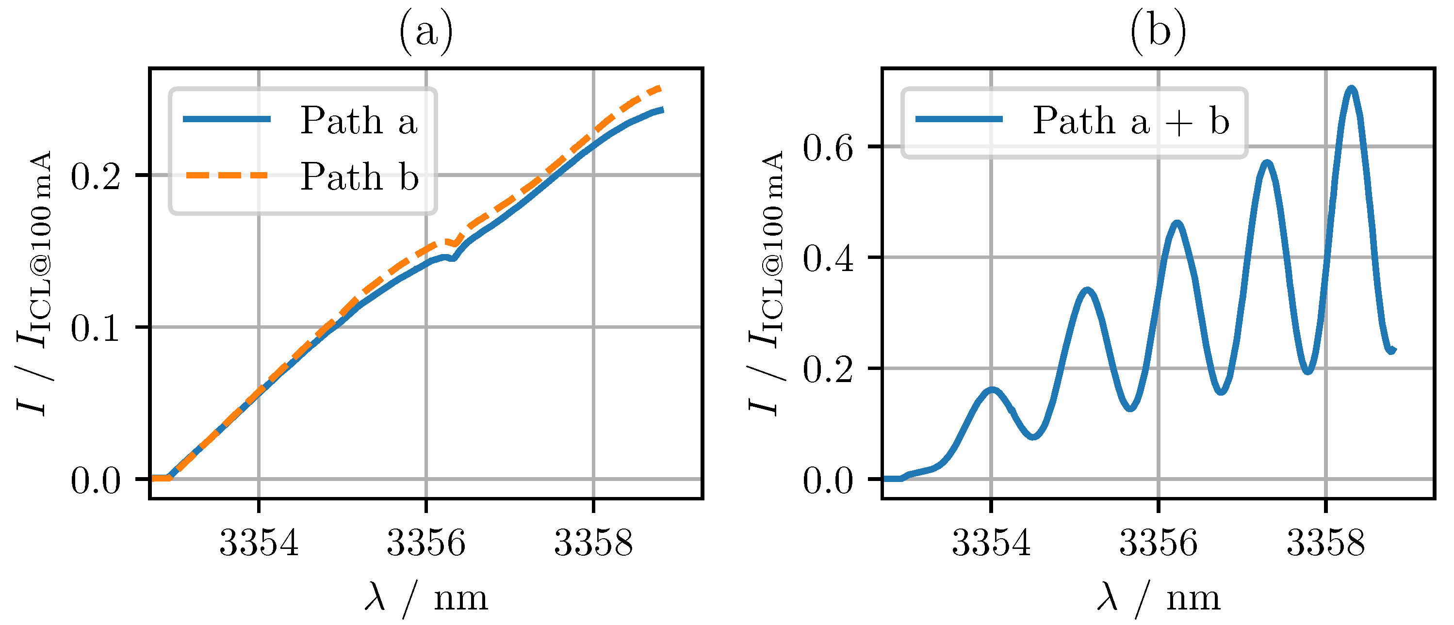
To obtain the individual intensities ${\widehat{I}}_{\mathrm{a}}$ and ${\widehat{I}}_{\mathrm{b}}$, we blocked the respective other beam inside the MZI; see Figure 3. The measured intensities ${\widehat{I}}_{\mathrm{a}}$ and ${\widehat{I}}_{\mathrm{b}}$ as a function of the emission wavelength during a linear increase of the laser current are shown in Figure 6a. The blue solid line represents the measured intensity ${\widehat{I}}_{\mathrm{a}}$, while the orange dashed line represents the measured intensity ${\widehat{I}}_{\mathrm{b}}$. The ICL threshold current was determined to be 35 mA for both intensities.

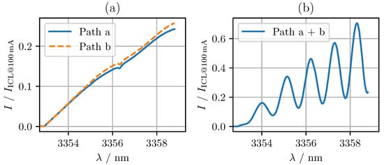
Figure 6. Measured intensities $\widehat{I}$, scaled with respect to the intensity at 100 mA laser current $I_{\mathrm{ICL}@100\mathrm{mA}}$: (a) beam intensities ${\widehat{I}}_{\mathrm{a}}$ and ${\widehat{I}}_{\mathrm{b}}$ separately; (b) interference of ${\widehat{I}}_{\mathrm{a}}$ and ${\widehat{I}}_{\mathrm{b}}$ generating ${\widehat{I}}_{\mathrm{MZI}}$.

The intensity values were normalized according to the intensity of the ICL at 100 mA, the highest current level applied in our measurements. The ICL intensity $I_{\mathrm{ICL}}$ could not be directly measured without modifying the experimental setup. Using Equation (11) and assuming that $\cos \left({\varphi }_{\mathrm{MZI}}\right){\eta }_{\mathrm{MZI}}=1$ and the interferometer is lossless, $I_{\mathrm{ICL}}$ was estimated by

$$I_{\mathrm{ICL}}={\widehat{I}}_{\mathrm{a}}+{\widehat{I}}_{\mathrm{b}}+2\sqrt{{\widehat{I}}_{\mathrm{a}}{\widehat{I}}_{\mathrm{b}}}.$$

(12)

The maximum intensities ${\widehat{I}}_{\mathrm{a}}$ and ${\widehat{I}}_{\mathrm{b}}$ corresponded to approximately a quarter of the original intensity of the laser $I_{\mathrm{ICL}}$, which was to be expected given that the two output intensities were not significantly disparate. The slight discrepancy in intensity observed between ${\widehat{I}}_{\mathrm{a}}$ and ${\widehat{I}}_{\mathrm{b}}$, as revealed in Figure 6a, can be attributed to the reflectivity of the beam splitters. The absorption line at approximately 3356.5 nm was caused by water vapor in the air.

The normalized intensity of the MZI output ${\widehat{I}}_{\mathrm{MZI}}$ with both interferometer arms in use is shown in Figure 6b.

By evaluating a pair of consecutive maxima or minima, the difference in the optical path length of the two interferometer arms $dn$ could be calculated

$$dn={\displaystyle \frac{{\lambda }_0{\lambda }_1}{{\lambda }_1-{\lambda }_0}}\mathrm{at}{\varphi }_{\Delta \lambda }=2\pi ,$$

(13)

with the wavelength-dependent phase change ${\varphi }_{\Delta \lambda }$, defined in Equation (7). Averaging over all pairs of minima and maxima yielded in this example a $dn$ of (10.55 ± 0.21) mm.

The interference’s efficiency factor could be determined from the measurements of ${\widehat{I}}_{\mathrm{a}}$, ${\widehat{I}}_{\mathrm{b}}$, and ${\widehat{I}}_{\mathrm{MZI}}$ entered into a rearranged variant of Equation (11)

$${\eta }_{\mathrm{MZI}}={\displaystyle \frac{|{\widehat{I}}_{\mathrm{MZI}}-{\widehat{I}}_{\mathrm{a}}-{\widehat{I}}_{\mathrm{b}}|}{2\sqrt{{\widehat{I}}_{\mathrm{a}}{\widehat{I}}_{\mathrm{b}}}}}\mathrm{at}{\varphi }_{\Delta \lambda }=0,\pi ,2\pi ,3\pi ,\dots$$

(14)

For our setup, we achieved a factor of ${\eta }_{\mathrm{MZI}}=0.51\pm 0.04$.

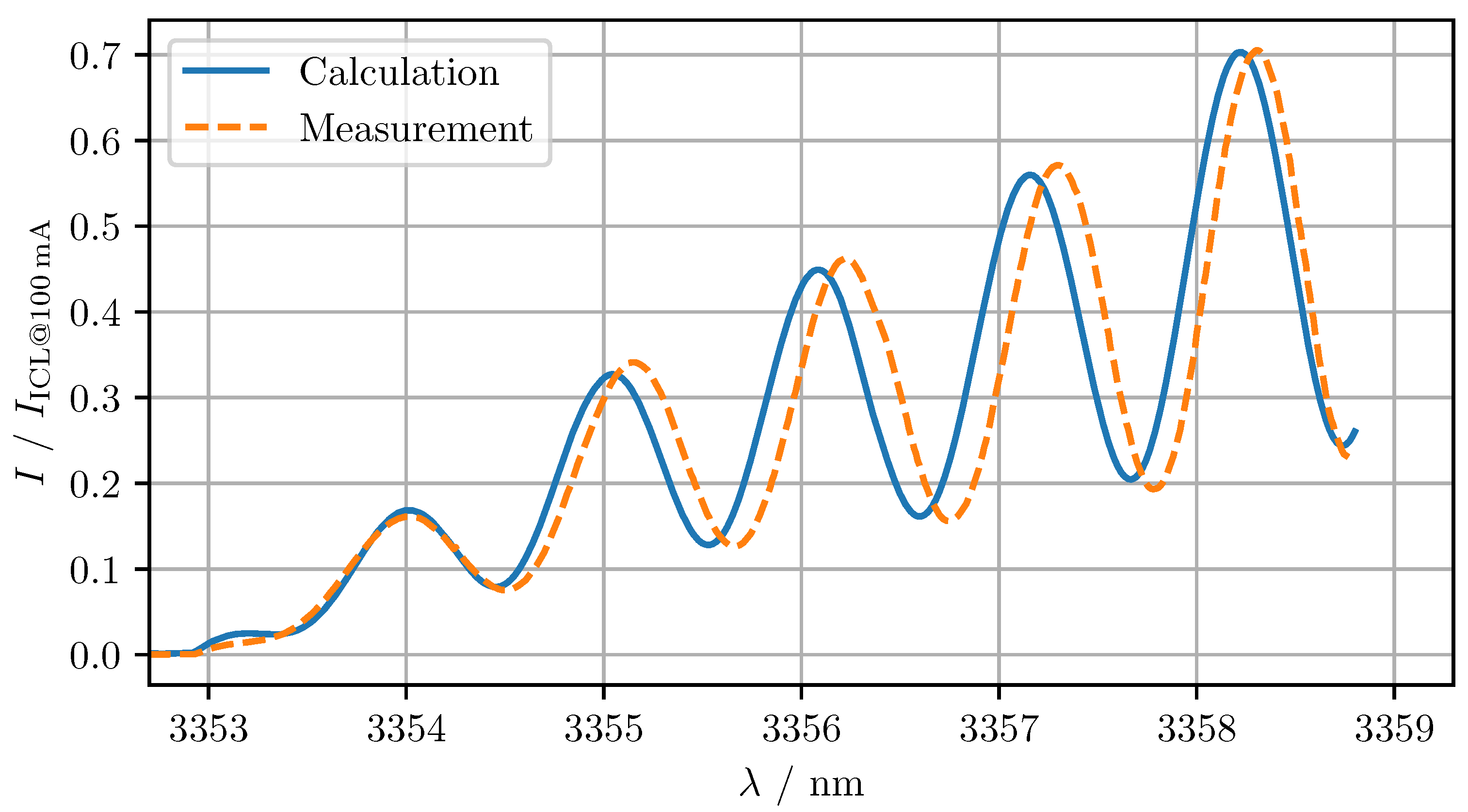
The model was evaluated by calculating $I_{\mathrm{MZI}}$ using Equation (11) with ${\widehat{I}}_{\mathrm{a}}$, ${\widehat{I}}_{\mathrm{b}}$, and ${\eta }_{\mathrm{MZI}}$ and comparing it to the actual ${\widehat{I}}_{\mathrm{MZI}}$ measurement. The results of the calculation and measurement are presented in Figure 7.

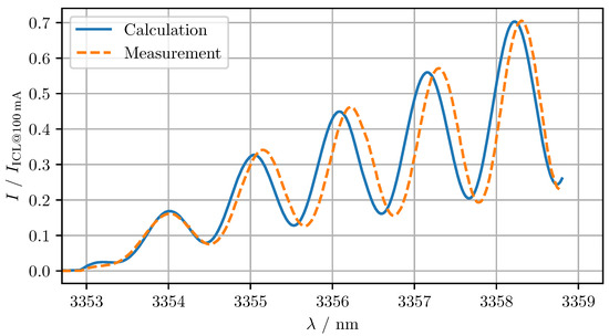
Figure 7. Measurement ${\widehat{I}}_{\mathrm{MZI}}$ and calculation $I_{\mathrm{MZI}}$ of the interferometer intensity of a laser current–wavelength sweep. For the calculation, $dn$ was set to 10.55 mm and ${\eta }_{\mathrm{MZI}}$ to 0.51.

3.1. Interferometrically Enhanced Intensity Modulation

In IE intensity modulation, the laser current is modulated to periodically switch between a local minimum (destructive interference) and the subsequent maximum (constructive interference) of the MZI. To obtain a sinusoidal intensity output, a triangular laser current must be used [14].

Figure 8 depicts the IE intensity modulation ${\widehat{I}}_{\mathrm{MZI}}$ in comparison to traditional intensity modulation with the same amplitude.

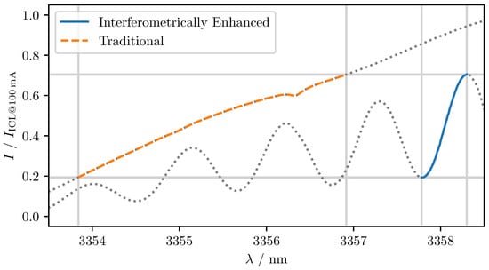
Figure 8. Traditional intensity modulation $I_{\mathrm{ICL}}$ and IE intensity modulation ${\widehat{I}}_{\mathrm{MZI}}$. Intensities scaled with respect to the intensity emitted at 100 mA laser current $I_{\mathrm{ICL}@100\mathrm{mA}}$.

As the change in intensity was considered to be the intensity modulation signal $\tilde{S}$, the normalized amplitude was calculated by

$$\tilde{S}={\displaystyle \frac{{\widehat{I}}_{\lambda }-{\widehat{I}}_{\lambda -\Delta \lambda }}{I_{\mathrm{ICL}@100\mathrm{mA}}}}$$

(15)

and its bias ${\overline{S}}_{\mathrm{int}}$ by

$$\overline{S}={\displaystyle \frac{{\widehat{I}}_{\lambda -\Delta \lambda }}{I_{\mathrm{ICL}@100\mathrm{mA}}}},$$

(16)

with the wavelength at constructive interference $\lambda$ and the residual wavelength modulation $\Delta \lambda$.

In the case of the example illustrated in Figure 8, a modulation with $\tilde{S}=0.51$ and $\overline{S}=0.19$ for both the IE and the traditional IE was selected. For the traditional IM, represented by the orange dashed line, a residual WM of $\Delta \lambda =$ 3.0758 nm was measured. For the IE IM, represented by the blue solid line, a residual WM of only $\Delta \lambda =$ 0.5187 nm was measured. This corresponds to a reduction of the residual WM by 83%. The gray dotted lines illustrate the intensity when the laser current and, consequently, the wavelength exceeded or fell below the intended modulation.

An increase in the path length difference d of the interferometer would further reduce the residual wavelength $\Delta \lambda$.

3.2. Interferometrically Enhanced Wavelength Modulation

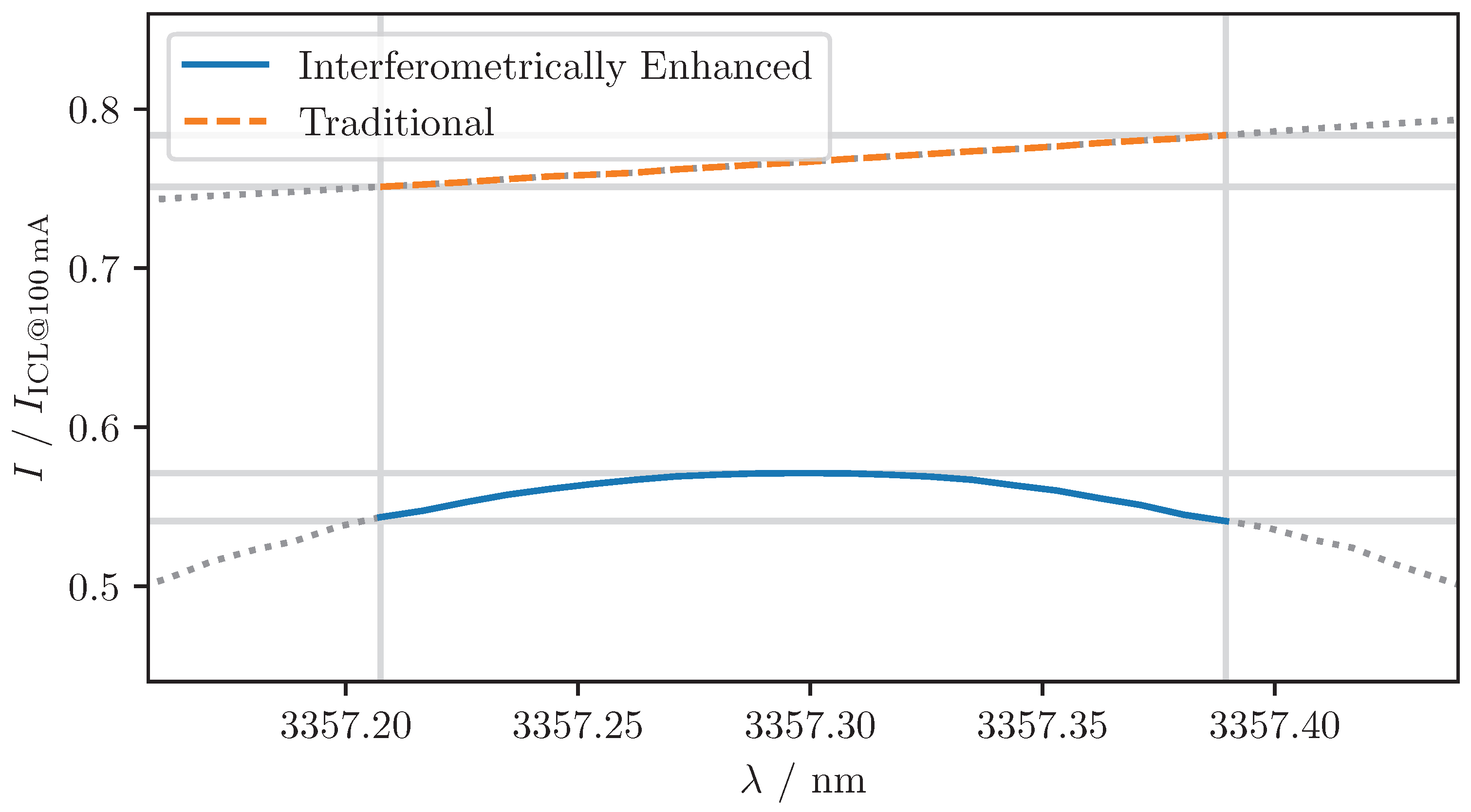
In the case of WM, the objective is to induce a wavelength shift and minimize the intensity change. In order to achieve the optimal IE wavelength modulation, it is necessary to identify the point of local interference, which is defined as the point at which the intensity $I_{\mathrm{MZI}}$ is at its maximum, but its derivative ${\displaystyle \frac{\mathrm{d}}{\mathrm{d}\lambda }}{I}_{\mathrm{MZI}}$ is equal to zero. A comparison between IE wavelength modulation and the traditional WM with the same amplitude is illustrated in Figure 9.

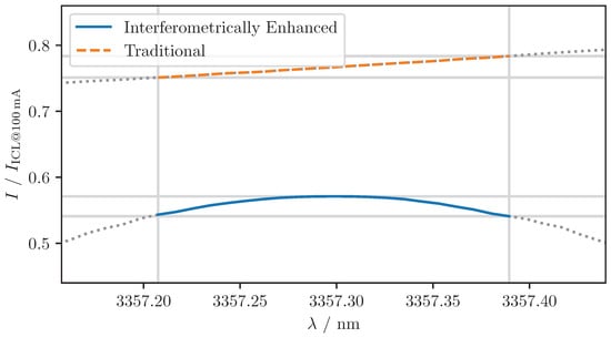
Figure 9. Traditional wavelength modulation $I_{\mathrm{ICL}}$ and IE wavelength modulation ${\widehat{I}}_{\mathrm{MZI}}$. Intensities scaled with respect to the intensity emitted at 100 mA laser current $I_{\mathrm{ICL}@100\mathrm{mA}}$.

In general, a reduction in the wavelength modulation depth results in a corresponding decrease in the residual intensity modulation. A reduction in path length difference $dn$ also results in a decrease in residual intensity modulation within IE wavelength modulation. In the case of the example illustrated in Figure 9, a modulation of $\Delta \lambda =$ 0.1812 nm was chosen. This resulted in a residual $\tilde{S}=0.0325$ and bias $\overline{S}=0.7512$ for the traditional modulation signal, represented by the orange dashed line, and a residual $\tilde{S}=0.0301$ and bias $\overline{S}=0.5434$ for the IE signal, represented by the blue solid line. The gray dotted lines illustrate the intensity when the laser current and, consequently, the wavelength exceeded or fell below the intended modulation.

For the derived signal, which is considered a noise factor in WMS, we obtained ${\displaystyle \frac{\mathrm{d}}{\mathrm{d}\lambda }}\tilde{S}\Delta \lambda =0.1785 \mathrm{n}{\mathrm{m}}^{-1}$ for traditional modulation and ${\displaystyle \frac{\mathrm{d}}{\mathrm{d}\lambda }}\tilde{S}\Delta \lambda =-0.0135 \mathrm{n}{\mathrm{m}}^{-1}$ for IE modulation.

It can be observed that the residual intensity modulation in IE wavelength modulation primarily contributes to the harmonics of the signal, but not to the fundamental signal itself. This allows for straightforward filtering via lock-in amplification.

4. Discussion and Conclusions

We introduced methods of interferometrically enhanced (IE) intensity and wavelength modulation for tunable diode laser spectroscopy. The proposed method reduces the entanglement between wavelength and intensity, which enables the measurement of spectra with higher spectral resolution.

To obtain continuous spectra, the phase of the MZI needs to be adjusted using either an electro-optic phase shifter, a piezo-driven mirror, or a tilting window; see Section 2.6. The tilting window was found to be highly stable in operation. The sinusoidal wavelength-dependent transmission of the MZI could also be used to generate a discrete spectrum with well-defined wavelength steps.

The calculation of the interference model presented in Section 2.4 was validated by our measurements in Section 3. The remaining differences between calculation and measurement can be attributed to a change in refractive index over the wavelength region, non-linearities of the laser emission wavelength, or small variations in the path length, for example, due to thermal expansion. Further investigation will be conducted on all of these factors.

An increase in the path length difference d of the interferometer favors IE intensity modulation, while a decrease favors IE wavelength modulation. A balanced d allows IE intensity modulation and IE wavelength modulation with a single setup, thus enabling the measurement of the signal amplitude $\tilde{S}$ and its derivative.

A different approach for reducing noise in TDLS uses an unbalanced Mach–Zehnder interferometer, whereby the second interferometer output is utilised as an intensity reference. By demodulating the transmission signal and reference signal, the noise can be suppressed [17].

The presented IE intensity modulation as well as IE wavelength modulation can be used in addition to conventional methods such as 2f modulation in TDLS to reduce the modulation residuals [18,19]. This does not aim to replace such methods, but rather to complement them.

Appendix A.1. Calculation of Uncertainties

The quantity obtained from a sample of N measurements $x_i$ where $i=1\dots N$ is defined as its mean value

$$\overline{x}={\displaystyle \frac{1}{N}}\sum _{i=1}^N{x}_i.$$

(A1)

with the uncertainty

$$\Delta x={\displaystyle \frac{s_x}{\sqrt{N}}},$$

(A2)

with the standard deviation

$$s_x=\sqrt{{\displaystyle \frac{1}{N-1}}\sum _{i=1}^N{(x_i-\overline{x})}^2}.$$

(A3)

Appendix A.2. Refraction at the Boundary between CaF₂ and Air

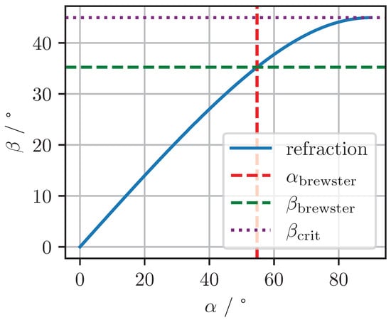
Figure A1. Angle of incidence $\alpha$ and angle of refraction $\beta$ of a refracted ray in a CaF₂ window.

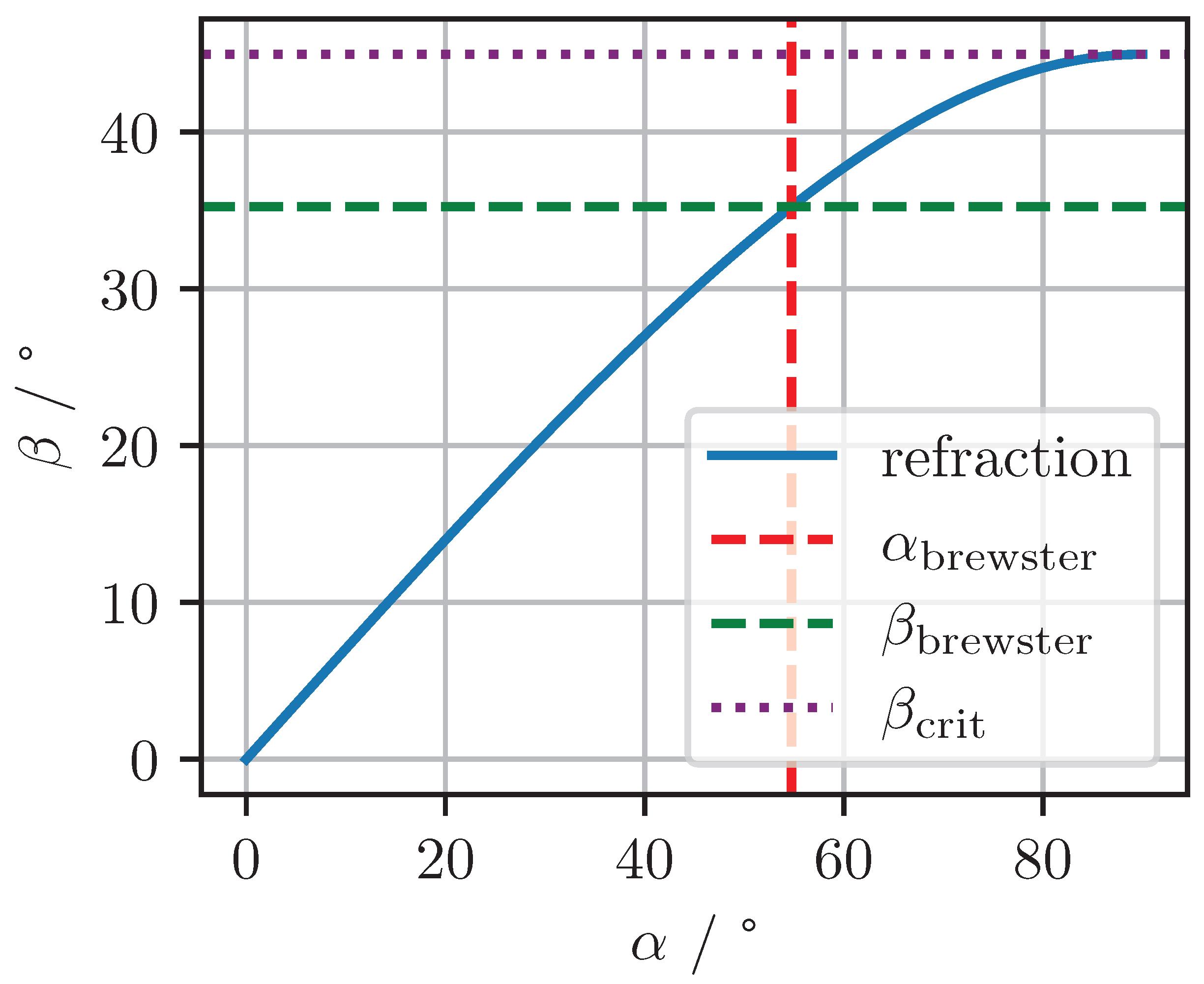
The refractive index of CaF₂ is $n_{{\mathrm{CaF}}_2}=1.4152$, at 3.35 μm and 24 °C [15,16].

The law of refraction at the boundary between two media is [13]

$$sin\left(\beta \right)=sin\left(\alpha \right){\displaystyle \frac{n_{\mathrm{air}}}{n_{{\mathrm{CaF}}_2}}}.$$

The Brewster angle in the case of external reflection is [13]

$${\alpha }_{\mathrm{Brewster}}={tan}^{-1}\left({\displaystyle \frac{n_{{\mathrm{CaF}}_2}}{n_{\mathrm{air}}}}\right)=54.755°$$

and in the case of internal reflection

$${\beta }_{\mathrm{Brewster}}={tan}^{-1}\left({\displaystyle \frac{n_{\mathrm{air}}}{n_{{\mathrm{CaF}}_2}}}\right)=35.245°.$$

The critical angle in the case of total internal reflection is [13]

$${\beta }_{\mathrm{crit}}={sin}^{-1}\left({\displaystyle \frac{n_{\mathrm{air}}}{n_{{\mathrm{CaF}}_2}}}\right)=44.958°.$$

References

- Ma, Y.; Hao, Q. State-of-the-Art Laser Spectroscopy and Its Applications: Volume II; Frontiers in Physics, Frontier Media SA: Lausanne, Switzerland, 2023. [Google Scholar] [CrossRef]
- Cardona, M. Modulation Spectroscopy of Semiconductors. In Advances in Solid State Physics; Madelung, O., Ed.; Pergamon: Oxford, UK, 1970; pp. 125–173. [Google Scholar] [CrossRef]
- Bruhns, H.; Saalberg, Y.; Wolff, M. Photoacoustic Hydrocarbon Spectroscopy Using a Mach-Zehnder Modulated Cw OPO. Sens. Transducers 2015, 188, 40. [Google Scholar]
- Lawetz, C.; Cartledge, J.; Rolland, C.; Yu, J. Modulation Characteristics of Semiconductor Mach-Zehnder Optical Modulators. J. Light. Technol. 1997, 15, 697–703. [Google Scholar] [CrossRef]
- Xu, S.; Ren, Z.; Dong, B.; Zhou, J.; Liu, W.; Lee, C. Mid-Infrared Silicon-on-Lithium-Niobate Electro-Optic Modulators Toward Integrated Spectroscopic Sensing Systems. Adv. Opt. Mater. 2023, 11, 2202228. [Google Scholar] [CrossRef]
- Bonfiglioli, G.; Trench, J. Signal Recovering in Wavelength Modulated Spectrometers. Opt. Commun. 1974, 10, 207–210. [Google Scholar] [CrossRef]
- Schilt, S.; Thévenaz, L.; Robert, P. Wavelength Modulation Spectroscopy: Combined Frequency and Intensity Laser Modulation. Appl. Opt. 2003, 42, 6728–6738. [Google Scholar] [CrossRef] [PubMed]
- Moses, E.I.; Tang, C.L. High-Sensitivity Laser Wavelength-Modulation Spectroscopy. Opt. Lett. 1977, 1, 115–117. [Google Scholar] [CrossRef] [PubMed]
- Montesinos-Ballester, M.; Deniel, L.; Koompai, N.; Nguyen, T.H.N.; Frigerio, J.; Ballabio, A.; Falcone, V.; Le Roux, X.; Alonso-Ramos, C.; Vivien, L.; et al. Mid-Infrared Integrated Electro-optic Modulator Operating up to 225 MHz between 6.4 and 10.7 Um Wavelength. ACS Photonics 2022, 9, 249–255. [Google Scholar] [CrossRef]
- Welkowsky, M.; Braunstein, R. A Double Beam Single Detector Wavelength Modulation Spectrometer. Rev. Sci. Instruments 1972, 43, 399–403. [Google Scholar] [CrossRef]
- Hariharan, P. Basics of Interferometry, 2nd ed.; Elsevier Academic Press: Amsterdam, The Netherlands; Boston, MA, USA, 2007. [Google Scholar]
- Born, M.; Wolf, E. Principles of Optics: Electromagnetic Theory of Propagation, Interference and Diffraction of Light, 7th ed.; Cambridge University Press: Cambridge, UK, 1999. [Google Scholar] [CrossRef]
- Saleh, B.E.A.; Teich, M.C. Fundamentals of Photonics; John Wiley & Sons: Hoboken, NJ, USA, 2019. [Google Scholar]
- Vervoort, S.; Saalberg, Y.; Wolff, M. Mach–Zehnder Modulator Output in Time and Frequency Domain – Calculation and Experimental Confirmation. Photonics 2023, 10, 337. [Google Scholar] [CrossRef]
- Malitson, I.H. A Redetermination of Some Optical Properties of Calcium Fluoride. Appl. Opt. 1963, 2, 1103–1107. [Google Scholar] [CrossRef]
- Polyanskiy, M.N. Refractiveindex.Info Database of Optical Constants. Sci. Data 2024, 11, 94. [Google Scholar] [CrossRef] [PubMed]
- Xu, L.; Hou, G.; Qiu, S.; Huang, A.; Zhang, H.; Cao, Z. Noise Immune TDLAS Temperature Measurement Through Spectrum Shifting by Using a Mach–Zehnder Interferometer. IEEE Trans. Instrum. Meas. 2021, 70, 7004009. [Google Scholar] [CrossRef]
- Bomse, D.S.; Stanton, A.C.; Silver, J.A. Frequency Modulation and Wavelength Modulation Spectroscopies: Comparison of Experimental Methods Using a Lead-Salt Diode Laser. Appl. Opt. 1992, 31, 718. [Google Scholar] [CrossRef] [PubMed]
- Li, J.; Du, Z.; An, Y. Frequency Modulation Characteristics for Interband Cascade Lasers Emitting at 3 μm. Appl. Phys. B 2015, 121, 7–17. [Google Scholar] [CrossRef]
Disclaimer/Publisher’s Note: The statements, opinions and data contained in all publications are solely those of the individual author(s) and contributor(s) and not of MDPI and/or the editor(s). MDPI and/or the editor(s) disclaim responsibility for any injury to people or property resulting from any ideas, methods, instructions or products referred to in the content. |
© 2024 by the authors. Licensee MDPI, Basel, Switzerland. This article is an open access article distributed under the terms and conditions of the Creative Commons Attribution (CC BY) license (https://creativecommons.org/licenses/by/4.0/).