Measured and Predicted Speckle Correlation from Diffractive Metasurface Diffusers

Abstract

Speckles are inherent in structured laser-based light projection using diffractive optics such as metasurfaces or diffractive optical elements (DOEs). One application of structured light is to provide illumination for machine vision and depth sensing. This is particularly attractive for mobile or low-power applications, where metasurfaces provide a compact, customizable solution, which can furthermore reach extreme field of illuminations. However, the speckles might limit detection capabilities by, e.g., lowering the detection range or providing false results. In this work, we present a series of measurements with matching simulations on a 70 × 50 degrees diffractive diffuser using different light sources (varying divergence angles + VCSEL array) to quantify the impact of speckles. We observe a qualitative agreement in speckle correlation between the measurements and the simulations and explain, in part using cross-correlation for analysis, why we do not observe the same speckle pattern between the measurements and the simulations. By performing extra simulations, we conclude that by only changing the light source, there is a limit to the reduction of the speckle contrast which, we can achieve, and, to reduce it further, alternative approaches such as changing the design method of the diffractive diffuser must be harnessed.

1. Introduction

Metasurface optical elements are of great interest in investigating various properties of light such as phase [1,2,3,4], polarization [3,5] and orbital angular momentum [1,6,7], but they also have been explored for industrial applications such as three-dimensional imaging [8,9] for and automotive light detection and ranging (Lidar) [10,11,12]. In such configurations, the illumination element known as a diffuser, which redistributes light into a target pattern, plays a key role in providing precise and efficient illumination, as shown in Figure 1. Compared to the refractive optical elements such as micro-lens arrays [13], which utilize geometric curvature to deflect light, subwavelength meta-atoms control the local phase delay based on the meta structures aspect ratio, thereby redirecting the light in desired directions. Metasurfaces are produced with semiconductor processes such as E-Beam Lithography [1,2,3,4] and CMOS [14,15,16,17].

Speckles arising from light’s coherent nature are commonly observed in almost all laser-based optical systems [18,19]. For illumination systems such as, for example Lidar, speckle reduction is important for high-precision 3D sensing. Furthermore, a long exposure of speckles to human eyes can lead to irritation and headaches [18]. To suppress the speckle effect, most of the research has focused on introducing dedicated mechanical movement [20,21], random vibrations [22,23], that in some instances are integrated with micro–electro–mechanical systems (MEMSs) [24,25]. For example, S. Kubota et al. observed speckle reduction by moving the diffuser device [21]. M.N. Akram et al. proposed introducing spatial and angular diversity by fast scanning micromirror [24]. J. W. Pan et al. used a vibrating symmetric diffuser to suppress speckles and maintain contrast [22]. H. A. Chen et al. demonstrated speckle reduction using deformable mirrors with diffusers in a laser pico-projector [20]. In 2024, N. Yang et al. reported a record-high efficiency speckle suppression in multimode fibers using cascaded cylindrical piezoelectric ceramics [26].

In addition, motionless systems are of increasing interest for industrial applications due to the requirement of robustness to failure tests, which are known as the so-called “solid-state” elements. For this purpose, H. Farrokhi et al. [27] studied electroactive micro-optics diffusers for tunable speckle reduction. Vladimir K. et al. [28] proposed a dynamic diffractive light modulator that was based on an electrically controlled spatial light modulator. C.K. Lo et al. [29] studied speckle reduction with a fast electrically tunable lens. Furthermore, another technique was developed to use a 2D binary code (e.g., Hadamard matrices) [18,30,31].

As an alternative to introducing randomness in the time domain, J.W. Goodman [19] and M.N. Akram [18] listed other possible degrees of freedom in speckle reduction, which include spectral diversity, polarization averaging, and multiple emitters. Vertical-cavity-surface-emitting lasers (VCSELs) [32,33] have attracted a lot of attention for industrial applications due to a high active area and thus, high emitting power. However, they also have a lower divergent angle compared to the edge-emitting laser (EEL). To directly design a high-quality diffuser for a divergent light source or VCSEL array requires full-wave simulation, such as FDTD, which is extremely expensive. It is therefore of interest if one can predict the behavior of a diffuser that is optimized for a simpler light source such as collimated light and simulate the effects on the profile and speckle pattern when illuminated with a more complex light source. If this is successful, we bypass the need to use expensive FDTD to design directly a complex light source. In this work, we investigate how the speckle varies with different illumination conditions and demonstrate that the speckles from a diffuser designed for a collimated beam can be reduced when illuminated by a divergent beam compared to a collimated beam and further reduced when illuminated by multiple such emitters. To understand the behavior, we analyze the speckle patterns of the diffuser to see if there is a quantitative agreement in speckle correlation between measurements and simulations.

2. Materials and Methods

For traditional diffractive optical elements (DOEs), the phase-map would be converted to heights, whereas the phase-map is replaced by meta-atoms of varying diameters for MOEs (Figure 2). The parameters of the diffuser design selected for generating the phase-map, such as the height of the pillars, lattice size and pillar diameter range, are selected to maximize the transmission of the meta-pillars in the periodic lattice while covering a 2-pi change in phase across the pillar diameter range. To investigate the effect of divergence of light and translation of an illumination source, the diffuser design selected for this study was optimized for illumination with collimated light to see to what degree speckle contrast could be reduced purely by changing the light source. For the present study, we chose to investigate the speckle patterns from a standard meta-optical element (MOE) diffractive area diffuser (Figure 1b), which generates a pattern with a moderate field of view (FoV) of 70 × 50 degrees. The FoV is relevant for many 3D sensing applications and at the same time easy to characterize and simulate using standard methods (Figure 3). The intensity profile is designed to compensate relative illumination in a receiving imaging system (Figure 1b). The pattern is generated by designing a phase-map using in-house code that can be considered an extension of the Gerchberg–Saxton algorithm [34].

2.1. Processing/Fabrication

A description of the processing/fabrication method used in this study can be found in ref [4].

2.2. Speckle Contrast Definition

In laser-based optical systems, speckles arising from coherent interference are commonly observed. To quantify the speckle level in an image, the speckle contrast value was proposed [18,20,21,22,27]

$$C={\displaystyle \frac{\sigma }{\mu }}$$

(1)

where $\sigma$ is the standard deviation, and $\mu$ is the mean value of an image. The speckle contrast is normally between 0 to 100%, except for the cases where the zero value dominates the image. Human eyes will not notice the speckles as long as the speckle contrast value is below 5% [22,24,35]. The speckle contrast definition is independent of wavelength and has mainly a relative meaning [35,36]. Thus, we use the same definition and target value for the infrared illumination (940 nm) of this study.

2.3. FFT Correlation Function Definition and Method of Use

To investigate how the speckle contrast and speckle pattern are linked, the speckle patterns produced under different illumination conditions were cross-correlated. The correlation function used in this paper, where z is the correlation value of two d-dimensional arrays x and y, is defined as follows [37]:

$$z\left[k\right]=\left(x \ast y\right)\left(k-N+1\right)=\sum _{l=0}^{‖x‖-1}{x}_l{y}_{l-k+N-1}^{*}$$

(2)

$$\begin{gathered} For k=\mathrm{0,1},\dots ,‖x‖+‖y‖-2 where ‖x‖ is the length of x, N= \\ and y_m is 0 when m is outside the range of y \end{gathered}$$

Due to the large dimension of the diffuser profile images, a fast Fourier transformation (FFT) was used to convolve the two images being compared to speed up the cross-correlation. For each of the cross-correlations performed, the output was the full discrete linear cross-correlation, and the peak value and position of the cross-correlation were extracted and compared to the expected location on the original image to validate that the correlation had been performed correctly. More details about the procedures used to validate the method of cross-correlation, including the results of the tests, can be found in Section 3.2.

2.4. Simulation Setup

We design the diffuser profile by the irradiance distribution defined on a plane in the far-field (assuming 1 m away from the metasurface), and the amplitude of the electric field after diffraction is given by the angular spectrum method [38,39,40],

$$E\left(\alpha ,\beta \right)=A\iint U(x,y)e^{-i2\pi (\alpha x+\beta y)}dxdy$$

(3)

where U is the electric field in the near-field, with its amplitude and phase interpolated by the pillar diameter according to the phase table, as depicted in Figure 2. A is constant, while α and β are the direction cosines. In this transform, a rectangular profile in the Cartesian coordinates will become barrel-shaped in the direction-cosine space. In this work, the diffuser is designed for a collimated beam or plane wave illumination, and the reference is a uniform irradiance distribution defined on a plane in the far-field [41]. To model the diffuser pattern by a divergent beam, for simplicity, a paraxial Gaussian beam model is used, and the full divergent angle is limited to 30 degrees in this study. When illuminated by multiple divergent emitters, the total diffuser pattern is an incoherent summation of diffuser patterns illuminated by different emitters. To make similar configurations as those in the experimental speckle measurements, the simulated diffraction images are transformed into the same grid as the measurements by interpolation.

2.5. Measurement Setup

The optical measurements of the diffusers were performed using the testing configuration shown in Figure 2. The primary measurement device is a “Radiant Vision Systems NIR Intensity Lens”, a radiometer camera for measuring the angular distribution of NIR emissions. The device is calibrated by the manufacturer for an operating wavelength of 940 nm. The glass wafer with the measured diffusers is placed on a translation stage, such that each diffuser can be maneuvered into the illumination beam path in sequence.

For each of the 3 distinct illumination configurations, as shown in Figure 2, we mechanically aligned the source to coincide with the optical axis of the radiometer camera and used a series of refractive and flat optics to control the illumination condition in the measurement plane. Images taken with the “Radiant Vision Systems NIR Intensity Lens” record the angular distribution of the diffused light when illuminated onto different locations on the diffuser: near the element center and at 4 other positions, each laterally shifted by 100 µm in the 4 cardinal directions, referred to as ‘translations’ in Section 3. Additionally, images are recorded as the distance from the diffusers to the illumination sources is varied over a range of 1 mm; this has the most relevance for divergent sources.

3. Results

3.1. Reduction of Speckle Contrast through an Increase in Divergence Angle of Input Beam, as Well as the Benefits of VCSEL Illumination in Reducing Speckle Contrast

The results discussed in this section are derived from the analysis of the diffuser profiles measured by the measurement setup described in Section 2.5. Some examples are shown in Figure 4b, alongside an image of the input beam which was used to illuminate the diffuser in the measurement setup. One can see the speckles which cover the profile of the diffuser profiles change in appearance according to the illumination condition, as well as the profile itself. The profile becomes more distorted the more the input light source deviates from the collimated beam for which the design was optimized.

The dependence of the of the speckle pattern upon lateral shifts of the diffuser relative to the light source was measured as shown in Figure 4a,b. For each type of input light source, the wafer was shifted to create a lateral offset between the position where the diffuser is illuminated and the center of the diffuser profile. A total of five measurements were taken that were subsequently analyzed, as described in Section 3.2. For each type of measurement conducted in this study, a corresponding simulated profile was also analyzed using the same methods to see if the behavior observed from analyzing the measured profiles could be predicted from the simulation.

3.1.1. Beam Shape, Divergence Angle and Multiple Emitters Can Be Used to Reduce Speckle Contrast

The measured diffuser profiles were analyzed to extract speckle contrast, magnitude and variation for different illumination conditions. The main results are presented in Figure 5 and Figure 6. We observe that the speckle contrast reduces when the divergence angle increases both in measurements and simulation (Figure 5), which is consistent with the experimental observations by J. W. Pan et al. [22]. The rate of decrease in speckle contrast ratio observed in measurements, however, differs from that in the simulation, where the speckle contrast has a much slower drop in magnitude, with an increase in the divergence angle. Different filters were applied to the simulated diffuser profiles to try and mimic the effect of the resolution of the detector used to capture the measured diffuser profiles (Figure 5); Despite this, the measured profiles achieve speckle contrast values below the lower limit of what was achieved in the simulated profiles. The reason for this discrepancy between simulations and measurements is due to the noise in the measurements which affects the speckle pattern of the diffuser profile, which will be discussed in further detail in Section 3.2.

A relevant light source for commercial applications is an array of vertical-cavity-surface-emitting laser (VCSEL) emitters integrated into a single chip. This source differs from single sources by consisting of an array of uncorrelated emitters, typically generating a doughnut-like beam profile rather than a Gaussian profile. Using a VCSEL array, we observe a speckle contrast below 10% (Figure 5). The VCSEL emitters have a divergence angle of 26 deg. From extrapolating the measurement data collected for the Gaussian beams with varying divergence angles, we would expect the VCSEL diffuser profile to achieve a speckle contrast below 10%. In addition, we investigated how the collective illumination pattern of the individual VCSEL sources affects the speckle contrast. A VCSEL, unlike a single-source Gaussian beam, consists of multiple emitters, arranged next to each other, most commonly in a hexagonal or rectangular array. We investigated through simulation how the number of emitters influence the speckle contrast. The simulation results show that the speckle contrast decreases exponentially, so that after about 100 emitters, the speckle contrast remained constant, as seen in Figure 6. Another difference between a VCSEL and a single Gaussian beam is that as the VCSEL consists of multiple emitters within an array, the emitters have a lateral offset between each other, which all contribute to the illumination of the diffuser profile. Therefore, to investigate if the superposition of the laterally offset diffuser profiles caused by the equal contributions of the lateral offset emitters would reduce the speckle contrast, the measured diffuser profiles illuminated with a lateral offset between the light source and the diffuser, as described in methods and materials, were added together to create one diffuser profile for each of the divergence angles tested and the speckle contrast extracted. The results of this study are shown in Figure 5 as red dots for the measurements taken with Gaussian beam and red stars for those measured with VCSEL. Here, we see that there is a reduction in the speckle contrast for all divergence angles when summing the diffuser profiles together rather than when the speckle contrast is extracted from the single emitter diffuser profiles, which are shown as the green dots in Figure 5 for Gaussian beam illumination and green stars for VCSEL illumination. Despite this, from simulation, as shown in Figure 6b, we see that by changing the distance between the multiple single Gaussian beam emitters used to illuminate the diffuser in the simulation (as well as the lateral offset between the illuminated diffuser profiles they would individually produce), the speckle contrast does not vary significantly. Finally, since the beam from the VCSEL consists of multiple modes [32,33], we expect better uniformity in the profile, which we also observe in Figure 7.

3.1.2. Variation of Speckle Contrast across Profile Decreases as Divergence Angle Increases

To identify which parts of the profile contributed the most to the speckle contrast, and thus better understand why it decreases when the divergence of the illumination angle is increased, the measured profiles were divided into subsections, as shown in Figure 7, and the speckle contrast within each subsection of the profile was calculated alongside the standard deviation (STD) of all the subdivisions of the profile. The main conclusion of this study was that not only did the speckle contrast decrease within each subdivision of the profile but the variance of the speckle contrast also decreased across the subdivisions when the divergence of the light source increased. Another observation of interest is that for the profiles illuminated with the single Gaussian beam, the subdivisions with the highest speckle contrast are located around the center of the profile, whereas when the diffuser is illuminated with a VCSEL, the subdivisions with the highest relative speckle contrast are located around the edge of the profile and are not symmetric. The most likely reason for the lack of symmetry is due to the divergence of the VCSEL, distorting the profile to such an extent that the grid includes some of the background noise in the calculation of the speckle contrast, therefore falsely inflating the values along one edge of the VCSEL-illuminated diffuser profile.

3.2. Cross-Correlation Study of Speckle Patterns Shows the Deterministic Nature of the Speckle Pattern We Observed in Simulation Is Lost in Measurements

To investigate how a lateral offset between the diffuser and the illumination source affects the speckle pattern and thereby understand if one can use this to an advantage in reducing the speckle contrast of a diffuser profile, a cross-correlation study was conducted, both with the collected measurement data and the corresponding simulated profiles of the diffusers, using the cross-correlation function described in Materials and Methods. Because the diffuser design consists of repetitions of a unit cell with the size of a few microns, and we illuminate an area larger than one unit cell both in measurement and simulation, we assume from theory that the speckle pattern is deterministic, and therefore any change that we see in the speckle pattern under different illumination is caused by the illumination itself, not by different parts of the design being illuminated.

3.2.1. Speckle Pattern Must Be Separated from Diffuser Profile to Track the Similarity between Speckles Obtained from Profiles with Different Illumination Conditions

To ensure that cross-correlation correctly identified and correlated the speckles in the diffuser, rather than the profile of the diffuser, the speckle pattern was separated from the profile through an FFT transformation, where a threshold was set to extract the low-frequency part contributions of the profile, which was then subtracted from the original diffuser profile so that only the high-frequency components, the speckle pattern itself, was left for cross-correlation with the other extracted speckle patterns. The data depicted in Figure 8 validate the method. In Figure 8a, cross-correlations are performed between the separated speckle pattern itself and the translated profiles, both with the same divergence angle of the light source. We see that the highest cross-correlation is with itself rather than with the translated profiles. The same is not true for Figure 8b, where we see the same analysis performed for the diffuser profile, in which the speckle pattern has not been separated from the diffuser profile. Here, we see no difference in the magnitude of the cross-correlation between the translated profiles, which indicates that the overall diffuser profile dominates the cross-correlation rather than the speckle pattern.

To further ensure that the cross-correlation algorithm successfully identified the correct location of maximum correlation, the algorithm was run across a ‘cutout’ of the diffuser profile and cross-correlated with the full profile to see if the algorithm correctly located the placement of the center of the cutout as the place of maximum cross-correlation between the cutout and the full profile. Figure 9 illustrates an example of how this was achieved, as well as the cross-correlation results of this autocorrelation when performed for the various translated profiles with varying cutout sizes.

The key takeaway here is that the cross-correlation trend was repeatable across cutout sizes and in each case, the location of the center of the cutout was correctly identified as the place of maximum cross-correlation. It should be noted that the magnitude of the peak cross-correlation value decreasing with a reduction in cutout size observed in Figure 9b is due to the decrease in the number of pixels being correlated.

Consequently, the cross-correlation is useful to extract the relative similarity between speckle patterns from the same diffuser, but under different illumination conditions. It is even able to extract a shift in the position of the maximum correlation when the input beam is shifted laterally relative to the diffuser.

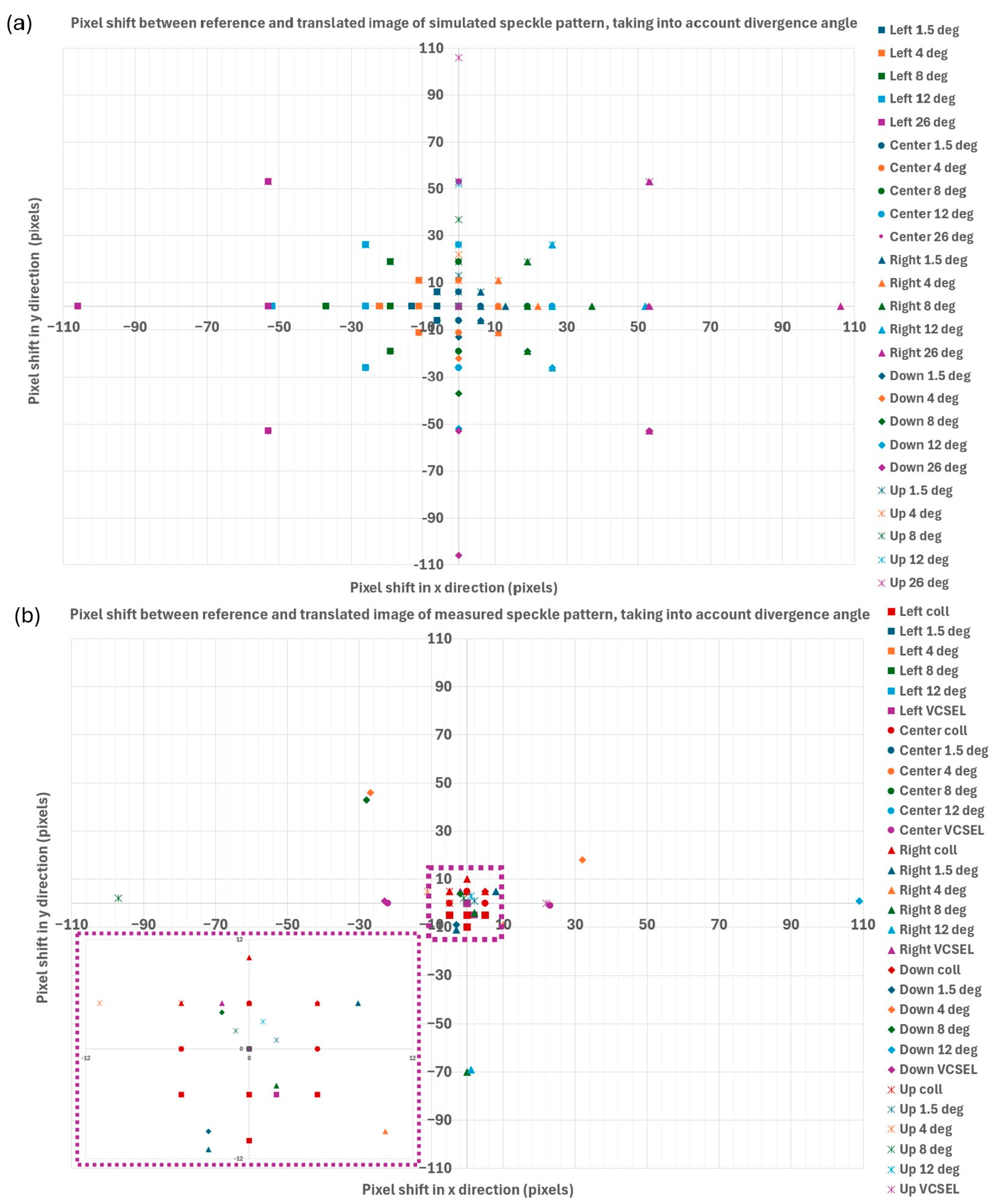
3.2.2. Simulated Speckle Patterns Show Systematic Shift According to Lateral Offset and Divergence of the Light Source, but the Shift Is Not Reproducible in the Analysis of Measured Speckle Patterns

Figure 10 and Figure 11 show the results of the cross-correlation study that was completed both for the simulated and measured speckle patterns, where for each of the different types of input beam tested, the translated speckle patterns with the same input light source were cross-correlated to each other, so that each was used as the reference pattern in the cross-correlation against the other translated speckle patterns, leading to a total of 25 cross-correlation results per illumination type. In Figure 10, we see from the simulation that the magnitude of the cross-correlation, regardless of the reference speckle pattern that is used, is highest when the speckle pattern is correlated with itself and decreases as the lateral difference between the reference speckle pattern and the translated speckle pattern that it is compared to increases. Interestingly, we see that while the trend is the same when the divergence angle of the light source is increased, the relative difference between the smallest and largest values of maximum correlation reduces. For the measured speckle patterns, we observe in Figure 10 that when these speckle patterns undergo the same analysis, the auto cross-correlation values vary more as the divergence angle increases. For a divergence angle of 1.5 degrees, we see that the magnitude of the cross-correlations between the speckle patterns of different translations is similar in both the simulations and the measurements. However, the ‘Left’ measured translation is an outlier when cross-correlated with the ‘center’ translation, as its cross-correlation magnitude is less than half of the other values. When not taking this outlier into account, we see a good correspondence with simulation, in that the larger the lateral difference between the light source and the diffuser, the smaller the cross-correlation becomes. When we compare the simulated cross-correlation results for the divergence angle of 12 degrees to the measured results, we see that again we obtain a good qualitative correspondence: the larger the lateral distance between the light source and the diffuser, the smaller the magnitude of the cross-correlation. It should be noted as well, however, that the quantitative magnitude of the cross-correlations from the measurements is lower than those expected from the simulations. Figure 10b demonstrates these qualitative matches more clearly.

When we compare the pixel shift obtained for the measured speckle patterns then apart from the collimated measurements, we do not observe a consistent trend between translation and the divergence of the input beam, unlike in the simulations. The possible reasons why we do not see the same trend in the measurements and the simulations are found in the discussion of this paper.

3.2.3. Cross-Correlation Rejects the Notion That the Detailed Simulated and Measured Speckles Patterns Can Be Related

From diffraction theory, we know that the speckle pattern a diffuser emits is deterministic when the light source is known [39,40]. We, therefore, cross-correlated the simulated and measure profiles to better understand the difference in behavior we observed in Figure 10 and Figure 11, both in terms of pixel shift and relative max cross-correlation values. Figure 12 shows that when we apply the cross-correlation between the simulated and measured speckle patterns with the same illumination and no lateral offset to the illumination source, the cross-correlation algorithm fails to locate the correct location where the simulated and measured speckle pattern should match up, given the same illumination condition. This is true both when the total speckle pattern and a smaller cutout of the simulated speckle pattern are cross-correlated with the total speckle pattern extracted from the measured profile. These results indicate that the speckle pattern extracted from the measured profile is too different from the simulated profile to be able to correctly cross-correlate the speckles.

4. Discussion

One of the main findings in this work is that, despite the speckle pattern being deterministic in simulation, we are not able to verify from cross-correlation analysis that the detailed speckle pattern is the same in the measurements. Several distinct reasons could help to explain why this is the case. In the measurements, it is assumed that the number of unit cells which are illuminated is greater than one for the speckle pattern to be deterministic, regardless of the offset between the illumination source and the diffuser. If less than one unit cell were illuminated, however, this would mean that the speckle pattern would lose its deterministic nature and we would not expect the pixel shifts observed in Figure 11 but rather more randomness in the size and direction of the shifts. In Figure 13, we see that when less than one unit cell is illuminated, but we are close to the size of one unit cell (~800 × 800 microns), for the most part, we see that we observe the same pixel shift pattern as observed when more than one unit cell is illuminated, but if the size of the illuminated area is reduced even further, then the pixel shifts increase in randomness. In the measurements, however, we do not illuminate such an extremely small size of the unit cell, meaning that it is more likely that there is another reason that causes randomness in the pixel shifts that we observe in the measurements.

Another possible reason for the difference in speckle pattern between the measurements and the simulations is that there was external noise, either caused by the measurements or fabrication defects, which added randomness to the speckle pattern in such a way that the changes in the speckle pattern according to the illumination divergence seen in the simulations were lost. To test this theory, the simulation cross-correlation study was repeated for different offsets and illumination divergence angles, where a Gaussian filter was applied on top of the speckle patterns, to see if this affected the pixel shift observed in Figure 11. As can be seen in Figure 14, the consistency in the pixel shifts observed in Figure 11 is lost, indicating that the measurements are too affected by noise for the cross-correlation to detect such sensitive changes in the speckle pattern. We do expect, however that the pixel shift is there in reality because of the decrease in speckle contrast that we see from Figure 5, where the sum of the translated profiles together gives a much smaller speckle contrast ratio compared to a single profile, as well as from Figure 15, which shows an example of a diffuser profile measured with a single Gaussian light source, compared to a profile constructed by adding five profiles together, where each profile was captured with a different lateral displacement between the illumination source and the MOE diffuser.

To ensure that the cross-correlation between the simulated and measured profile did not fail due to the conditions during the measurements being different than expected, such as the divergence angle being different than what was recorded or the diffuser profile being flipped compared to the simulation, variations of the simulated diffuser profile were compared to the same measured profile, where the divergence angle, offset, beam size, filtering and rotation of the simulated profile were modified to try and improve the cross-correlation with the measured profile, yet none led to the cross-correlation being able to correctly identify the location where the speckle should be if the simulated and measured speckle pattern were the same. To verify if the reason for the failure of the cross-correlation was due to the extraction method of the speckle pattern, an alternative FFT method, where a high-frequency filter was used to directly extract the higher-frequency speckle pattern from the diffuser profile, and the same cross-correlation study was performed, but it still failed to positively identify the correct location of the speckle pattern when comparing the simulated and measured speckle patterns. It should also be added that for all cross-correlation studies between the measurements and simulations, the grid size was kept the same to ensure that the size of the pixels, and therefore the corresponding speckles in terms of pixels, was the same between the measurements and the simulations.

Furthermore, to verify the impact of polarization, measurements with a collimated source were performed, where the polarization state was controlled, so that measurements were captured for two orthogonally polarized linear states and circular polarization. From these measurements, the speckle contrast was calculated, and the cross-correlation between the orthogonal linearly polarized illumination conditions was compared. The speckle pattern was measured for five times for each polarization. The average speckle contrast of the two individual orthogonally opposed linear polarizations was found to be 62.7% and 51.4%, with a standard deviation of 1.8% and 2.06%, respectively, while for the circular polarization, the speckle contrast was found to be 62.3%, with a standard deviation of 1.75%. These results show that for the diffuser design investigated in this study, polarization has a moderate but detectable impact on the speckle contrast. For the cross-correlation comparison, however, the polarization state has a large effect on the speckle pattern. When comparing the magnitude of the cross-correlation to the auto cross-correlation of one of the polarizations, the magnitude of the cross-correlation was found to be within 5% of each other, whereas for the other polarization, there was a difference of 50%, which indicates that polarization has a strong effect on the speckle pattern in the diffuser.

Finally, to compare the advantages and disadvantages of the speckle reduction method investigated in this paper, we include

Table 1. This table shows the advantages and disadvantages of different methods of speckle suppression.

Method of Reducing Speckle Contrast	Advantages	Disadvantages
Large divergence angle (including VCSEL illumination)	Effective at reducing speckle contrast down to 6%, as demonstrated in Figure 5	If the diffuser is not optimized for divergent light sources, the profile shape is blurred, as shown in Figure 4
Increased number of emitters in VCSEL [18,19]	Up to 100 emitters, we see an improvement, as shown in Figure 6	For more than 100 emitters, we do not see a significant improvement
Integration of MEMS [22,23]	Demonstrated to reduce speckle contrast up to 43.08% in the case of free space geometry [23] Good agreement between measurements and simulations for speckle reduction [23]	The method described in [23] is highly dependent on the height of the diffuser design: If it has large height fluctuations, the autocorrelation function of the reflected wave is narrower than that of the surface height, which reduces the speckle reduction. Height variation in the design must be carefully optimized to reduce the speckle itself and is limited by the fabrication process; if the height difference is not correct (λ/2), the autocorrelation function of the reflected wave becomes significantly broad
Random vibration [20,21]	In the system proposed in Ref [20], speckle contrast is reduced By temporally averaging the diffuser by placing it on a tuning forkRef [21] demonstrates a reduction in speckle contrast	For application, the system proposed in Ref [20] requires not only an external source to introduce vibrations but also two separate diffuser elements. The proposal seen in Ref [21] is also inconvenient for application that require compact systems
Mechanical motion [18,19]	The system proposed is a combination of a depolarizing screen, Galvano scan, dual polarizations and a moving diffuser to reduce speckle contrast of a laser source from 97% to 7% Ref [18].	Moving diffuser means that a mechanical component must be added to the illumination module to reduce the speckle contrast of the diffuser, making the module less compact

to compare it with other methods used in recent publications to reduce speckle contrast.

5. Conclusions

This work demonstrates not only that the speckle contrast of a diffuser profile produced by a MOE diffuser element can be reduced by increasing the divergence of the light source, but also that this approach reduces the variation of the speckle contrast across the diffuser profile. However, by simply increasing the divergence of the light source, there is a limit to which one can reduce the speckle contrast. To reduce it even further, below 10%, we have shown that a VCSEL light source can be used. Other than the large divergence angle of the VCSEL used in this study, we have shown through simulation, that the number of emitters in a VCSEL array also contributes to the speckle pattern up to 100 emitters, after which increasing the number of emitters in a VCSEL array will no longer help to reduce the speckle contrast. From the simulation, we also see that for VCSEL illumination, the distance between the emitters in the range tested does not have a significant impact on the speckle contrast of the diffuser profile.

The speckle patterns shift according to the position of the input beam, but the significance of the shift decreases with an increased divergence of the light source in the measurements. In the simulations, we see that the size of the shift in profile increases with the divergence of the light source, and it is very repeatable, as demonstrated in Figure 11. When a Gaussian filter is applied to the simulated speckle pattern, however, the repeatability and quantized steps in the shift previously observed vanish. This indicates that noise in the measurements, such as the Gaussian filter applied to the simulated speckle pattern, may be masking the shift in speckle pattern between illumination offsets. The fact that we see the reduction in speckle contrast when summing the measured translated profiles together, compared to the individual translated profiles, tells us that there is a shift between the translated profiles, just not one that is significant enough for the cross-correlation study to be able to identify it. Another key finding of this paper is that we observe a qualitative match between the simulations and the measurements. The cross-correlation value decreases as the lateral distance between the speckle patterns being cross-correlated is increased. This is a significant finding, as it gives evidence that the speckle pattern behavior observed in the simulations can be reproduced in the measurements, although the detailed speckle pattern cannot be reproduced by the simulation.

The speckle pattern is extremely sensitive to even minute changes in both the illumination source, the tolerances in the fabricated metasurface structure and the alignment between the light source and the diffuser. In the experimental setup, the control over these parameters is not sufficient to accurately predict the detailed speckle pattern.

To improve on the match between the simulations and the measurements, therefore, measures should be taken to either include these factors in the comparison or eliminate them as sources of uncertainty in the measured data. If this is achieved, there is great potential for improved applications in the future. One such example is non-invasive imaging through opaque surfaces, as seen in Ref. [42], that could take advantage of being able to predict the speckle pattern of a diffuser.

References

1. Ren, H.; Fang, X.; Jang, J.; Bürger, J.; Rho, J.; Maier, S.A. Complex-Amplitude Metasurface-Based Orbital Angular Momentum Holography in Momentum Space. Nat. Nanotechnol. 2020, 15, 948–955. [Google Scholar] [CrossRef] [PubMed]
2. Khorasaninejad, M.; Capasso, F. Metalenses: Versatile Multifunctional Photonic Components. Science 2017, 358, eaam8100. [Google Scholar] [CrossRef] [PubMed]
3. Balthasar Mueller, J.P.; Rubin, N.A.; Devlin, R.C.; Groever, B.; Capasso, F. Metasurface Polarization Optics: Independent Phase Control of Arbitrary Orthogonal States of Polarization. Phys. Rev. Lett. 2017, 118, 113901. [Google Scholar] [CrossRef]
4. Egede Johansen, V.; Gür, U.M.; Martínez-Llinás, J.; Fly Hansen, J.; Samadi, A.; Skak Vestergaard Larsen, M.; Nielsen, T.; Mattinson, F.; Schmidlin, M.; Mortensen, N.A.; et al. Nanoscale Precision Brings Experimental Metalens Efficiencies on Par with Theoretical Promises. Commun. Phys. 2024, 7, 123. [Google Scholar] [CrossRef]
5. Chen, W.T.; Zhu, A.Y.; Capasso, F. Flat Optics with Dispersion-Engineered Metasurfaces. Nat. Rev. Mater. 2020, 5, 604–620. [Google Scholar] [CrossRef]
6. Ren, H.; Briere, G.; Fang, X.; Ni, P.; Sawant, R.; Héron, S.; Chenot, S.; Vézian, S.; Damilano, B.; Brändli, V.; et al. Metasurface Orbital Angular Momentum Holography. Nat. Commun. 2019, 10, 2986. [Google Scholar] [CrossRef]
7. Sroor, H.; Huang, Y.-W.; Sephton, B.; Naidoo, D.; Vallés, A.; Ginis, V.; Qiu, C.-W.; Ambrosio, A.; Capasso, F.; Forbes, A. High-Purity Orbital Angular Momentum States from a Visible Metasurface Laser. Nat. Photonics 2020, 14, 498–503. [Google Scholar] [CrossRef]
8. Jing, X.; Li, Y.; Li, J.; Wang, Y.; Huang, L. Active 3D Positioning and Imaging Modulated by Single Fringe Projection with Compact Metasurface Device. Nanophotonics 2023, 12, 1923–1930. [Google Scholar] [CrossRef]
9. Tan, S.; Yang, F.; Boominathan, V.; Veeraraghavan, A.; Naik, G.V. 3D Imaging Using Extreme Dispersion in Optical Metasurfaces. ACS Photonics 2021, 8, 1421–1429. [Google Scholar] [CrossRef]
10. Lio, G.E.; Ferraro, A. LIDAR and Beam Steering Tailored by Neuromorphic Metasurfaces Dipped in a Tunable Surrounding Medium. Photonics 2021, 8, 65. [Google Scholar] [CrossRef]
11. Li, N.; Ho, C.P.; Xue, J.; Lim, L.W.; Chen, G.; Fu, Y.H.; Lee, L.Y.T. A Progress Review on Solid-State LiDAR and Nanophotonics-Based LiDAR Sensors. Laser Photonics Rev. 2022, 16, 2100511. [Google Scholar] [CrossRef]
12. Park, J.; Jeong, B.G.; Kim, S.I.; Lee, D.; Kim, J.; Shin, C.; Lee, C.B.; Otsuka, T.; Kyoung, J.; Kim, S.; et al. All-Solid-State Spatial Light Modulator with Independent Phase and Amplitude Control for Three-Dimensional LiDAR Applications. Nat. Nanotechnol. 2021, 16, 69–76. [Google Scholar] [CrossRef]
13. Yuan, W.; Li, L.-H.; Lee, W.-B.; Chan, C.-Y. Fabrication of Microlens Array and Its Application: A Review. Chin. J. Mech. Eng. 2018, 31, 16. [Google Scholar] [CrossRef]
14. Xu, Z.; Dong, Y.; Tseng, C.-K.; Hu, T.; Tong, J.; Zhong, Q.; Li, N.; Sim, L.; Lai, K.H.; Lin, Y.; et al. CMOS-Compatible All-Si Metasurface Polarizing Bandpass Filters on 12-Inch Wafers. Opt. Express 2019, 27, 26060–26069. [Google Scholar] [CrossRef] [PubMed]
15. Hu, T.; Zhong, Q.; Li, N.; Dong, Y.; Xu, Z.; Fu, Y.H.; Li, D.; Bliznetsov, V.; Zhou, Y.; Lai, K.H.; et al. CMOS-Compatible a-Si Metalenses on a 12-Inch Glass Wafer for Fingerprint Imaging. Nanophotonics 2020, 9, 823–830. [Google Scholar] [CrossRef]
16. Park, J.-S.; Zhang, S.; She, A.; Chen, W.T.; Lin, P.; Yousef, K.M.A.; Cheng, J.-X.; Capasso, F. All-Glass, Large Metalens at Visible Wavelength Using Deep-Ultraviolet Projection Lithography. Nano Lett. 2019, 19, 8673–8682. [Google Scholar] [CrossRef]
17. Park, J.-S.; Lim, S.W.D.; Amirzhan, A.; Kang, H.; Karrfalt, K.; Kim, D.; Leger, J.; Urbas, A.; Ossiander, M.; Li, Z.; et al. All-Glass 100 Mm Diameter Visible Metalens for Imaging the Cosmos. ACS Nano 2024, 18, 3187–3198. [Google Scholar] [CrossRef]
18. Akram, M.N.; Chen, X. Speckle Reduction Methods in Laser-Based Picture Projectors. Opt. Rev. 2016, 23, 108–120. [Google Scholar] [CrossRef]
19. Goodman, J.W. Speckle Phenomena in Optics: Theory and Applications; Roberts and Company Publishers: Greenwood Village, CO, USA, 2007; ISBN 978-0-9747077-9-2. [Google Scholar]
20. Chen, H.-A.; Pan, J.-W.; Yang, Z.-P. Speckle Reduction Using Deformable Mirrors with Diffusers in a Laser Pico-Projector. Opt. Express 2017, 25, 18140–18151. [Google Scholar] [CrossRef] [PubMed]
21. Kubota, S.; Goodman, J. Very Efficient Speckle Contrast Reduction Realized by Moving Diffuser Device. Appl. Opt. 2010, 49, 4385–4391. [Google Scholar] [CrossRef]
22. Pan, J.-W.; Shih, C.-H. Speckle Reduction and Maintaining Contrast in a LASER Pico-Projector Using a Vibrating Symmetric Diffuser. Opt. Express 2014, 22, 6464–6477. [Google Scholar] [CrossRef] [PubMed]
23. Mohamed, M.; Qianli, M.A.; Flannigan, L.; Xu, C.-Q. Laser Speckle Reduction Utilized by Lens Vibration for Laser Projection Applications. Eng. Res. Express 2019, 1, 015036. [Google Scholar] [CrossRef]
24. Akram, M.N.; Tong, Z.; Ouyang, G.; Chen, X.; Kartashov, V. Laser Speckle Reduction Due to Spatial and Angular Diversity Introduced by Fast Scanning Micromirror. Appl. Opt. 2010, 49, 3297. [Google Scholar] [CrossRef] [PubMed]
25. Tran, T.-K.-T.; Subramaniam, S.; Le, C.; Kaur, S.; Kalicinski, S.; Ekwińska, M.; Halvorsen, E.; Akram, M. Design, Modeling, and Characterization of a Microelectromechanical Diffuser Device for Laser Speckle Reduction. J. Microelectromech. Syst. 2014, 23, 117–127. [Google Scholar] [CrossRef]
26. Yang, N.; Li, Z.; Li, F.; Lang, T.; Guan, X. Record-High Efficiency Speckle Suppression in Multimode Fibers Using Cascaded Cylindrical Piezoelectric Ceramics. Photonics 2024, 11, 234. [Google Scholar] [CrossRef]
27. Farrokhi, H.; Rohith, T.M.; Boonruangkan, J.; Han, S.; Kim, H.; Kim, S.-W.; Kim, Y.-J. High-Brightness Laser Imaging with Tunable Speckle Reduction Enabled by Electroactive Micro-Optic Diffusers. Sci. Rep. 2017, 7, 15318. [Google Scholar] [CrossRef]
28. Kartashov, V.; Akram, M.N. Speckle Suppression in Projection Displays by Using a Motionless Changing Diffuser. J. Opt. Soc. Am. A 2010, 27, 2593. [Google Scholar] [CrossRef]
29. Lo, C.-K.; Pan, J.-W. Speckle Reduction with Fast Electrically Tunable Lens and Holographic Diffusers in a Laser Projector. Opt. Commun. 2020, 454, 124301. [Google Scholar] [CrossRef]
30. Gao, W.; Ma, S.; Chen, X. Speckle Reduction in Line Scan Laser Display System by Static Diffuser with 2D Binary Code. Chin. Opt. Lett. 2012, 10, 4. [Google Scholar] [CrossRef]
31. Trisnadi, J.I. Hadamard Speckle Contrast Reduction. Opt. Lett. 2004, 29, 11–13. [Google Scholar] [CrossRef]
32. Seurin, J.-F.; Xu, G.; Khalfin, V.; Miglo, A.; Wynn, J.D.; Pradhan, P.; Ghosh, C.L.; D’Asaro, L.A. Progress in High-Power High-Efficiency VCSEL Arrays. In Vertical-Cavity Surface-Emitting Lasers XIII; Choquette, K.D., Lei, C., Eds.; SPIE: San Jose, CA, USA, 2009; p. 722903. [Google Scholar]
33. Seurin, J.-F.; Ghosh, C.L.; Khalfin, V.; Miglo, A.; Xu, G.; Wynn, J.D.; Pradhan, P.; D’Asaro, L.A. High-Power High-Efficiency 2D VCSEL Arrays. In Vertical-Cavity Surface-Emitting Lasers XII; Lei, C., Guenter, J.K., Eds.; SPIE: San Jose, CA, USA, 2008; p. 690808. [Google Scholar]
34. Gerhberg, R.; Saxton, W. A Practical Algorithm for the Determination of Phase from Image and Diffraction Plane Picture. Optik 1972, 35, 237–246. [Google Scholar]
35. Furukawa, A.; Ohse, N.; Sato, Y.; Imanishi, D.; Wakabayashi, K.; Ito, S.; Tamamura, K.; Hirata, S. Effective Speckle Reduction in Laser Projection Displays. In Proceedings of the Emerging Liquid Crystal Technologies III; SPIE: San Jose, CA, USA, 2008; Volume 6911, pp. 183–189. [Google Scholar]
36. Roelandt, S.; Meuret, Y.; Craggs, G.; Verschaffelt, G.; Janssens, P.; Thienpont, H. Standardized Speckle Measurement Method Matched to Human Speckle Perception in Laser Projection Systems. Opt. Express 2012, 20, 8770. [Google Scholar] [CrossRef]
37. Virtanen, P.; Gommers, R.; Oliphant, T.E.; Haberland, M.; Reddy, T.; Cournapeau, D.; Burovski, E.; Peterson, P.; Weckesser, W.; Bright, J.; et al. SciPy 1.0: Fundamental Algorithms for Scientific Computing in Python. Nat. Methods 2020, 17, 261–272. [Google Scholar] [CrossRef] [PubMed]
38. O’Shea, D.C. Diffractive Optics: Design, Fabrication, and Test; SPIE Press: San Jose, CA, USA, 2004; ISBN 978-0-8194-5171-2. [Google Scholar]
39. Matsushima, K. Shifted Angular Spectrum Method for Off-Axis Numerical Propagation. Opt. Express 2010, 18, 18453–18463. [Google Scholar] [CrossRef] [PubMed]
40. Zhao, Y.; Cao, L.; Zhang, H.; Kong, D.; Jin, G. Accurate Calculation of Computer-Generated Holograms Using Angular-Spectrum Layer-Oriented Method. Opt. Express 2015, 23, 25440–25449. [Google Scholar] [CrossRef]
41. Harvey, J.E.; Vernold, C.L.; Krywonos, A.; Thompson, P.L. Diffracted Radiance: A Fundamental Quantity in Nonparaxial Scalar Diffraction Theory. Appl. Opt. 1999, 38, 6469–6481. [Google Scholar] [CrossRef] [PubMed]
42. Bertolotti, J.; van Putten, E.G.; Blum, C.; Lagendijk, A.; Vos, W.L.; Mosk, A.P. Non-Invasive Imaging through Opaque Scattering Layers. Nature 2012, 491, 232–234. [Google Scholar] [CrossRef]
Figure 1. (a) Three examples of how a diffuser can be used under different illumination conditions to create a large area of illumination that, in this case, is projected onto a screen. (b) Two examples of measured diffuser profiles from diffusers that NIL Technology has produced, demonstrating how depending on the design of the diffuser, custom shapes of profiles can be achieved. (c) A schematic of a potential application of a diffuser. In this case, the diffuser is part of a Lidar system used by the car to detect objects around it when driving, such as a person on a bicycle in this case.
Photonics 11 00845 g001
Figure 2. The simulated phase and transmission of the cylindrical a-Si meta-pillars used to translate the phase-map for the diffuser design into meta-pillars. The pillars all have a height of 500 nm and are situated in a 400 nm square lattice on top of a glass substrate.
Photonics 11 00845 g002
Figure 3. (a) A schematic of the alignment between the radiometer camera, the wafer containing the diffuser element and the optical setup used to illuminate the diffuser. (b) The three different optical setup configurations used to collect measurement data for this paper to compare how the speckle contrast changes under different illumination conditions. Config 1: VCSEL illumination. The VCSEL is modulated at 400 Hz with a 4% duty cycle. A set of relay lenses is used to illuminate the element plane from about 2–3 mm distance. Config 2: Collimated Beam Laser Diode. The mount is temperature controlled to 25 °C and operated with a current of 190 mA. The beam diameter is controlled with 2 lenses to achieve an approximate size of 1 mm. The source has linear polarization upon emission, so in some measurements, a waveplate is included to compare against circular polarization. Config 3: Divergent Beam Laser Diode. With the addition of a refractive lens to the configuration for the collimated beam (Config 2), the light is made to diverge from a point, at 1–2 mm from the wafer plane. The divergence can be selected with an adjustable iris, ranging from approximately 1 degree, up to 12 degrees full angle. An image of the setup is shown below Config 1.
Photonics 11 00845 g003
Figure 4. (a) A schematic of the measurement setup used to record the diffuser profiles from the side, including an arrow indicating the lateral offset, which was induced for 80% of the measurements between the diffuser and the illumination source by moving the wafer so that the center of the diffuser was not aligned with the center of the input beam profile. (b) A schematic of the illumination of the diffuser as seen from above, depending on the lateral offset between the illumination source and the diffuser. The figure denotes all five types of ‘translations’ that were recorded for each type of illumination source used on the diffuser. ‘U’, ‘L’, ‘C’, ‘R’ and ‘D’ denote ‘up’, ‘left’, ‘center’, ‘right’ and ‘down’, which are the directions in which the position of the illumination of the diffuser profile is compared to the center of the diffuser itself. (c) Examples of the input beams used in this paper, including their divergence angle for the single Gaussian beam light source, as well as the corresponding diffuser profile which they produced.
Photonics 11 00845 g004
Figure 5. (a) shows the speckle contrast of the diffuser profile as a function of the divergence angle of the illumination source, both from measurements and the simulation. Error bars are only present on the data points where a standard deviation from multiple data points could be calculated. (bd) The simulated diffuser profiles of varying divergence angles, together with their corresponding measured profiles to their right.
Photonics 11 00845 g005
Figure 6. (a) The simulated speckle contrast of a diffuser that is illuminated with a varying number of single Gaussian emitters as an approximation of a VCSEL array. One can observe from this subfigure that there is a limit to which the speckle contrast can be reduced by solely increasing the number of emitters. Even when the number of emitters is more than 100, the speckle contrast is higher than what is extracted from the measurements. Subfigure (b) shows how the distance between the multiple emitters used to illuminate the diffuser affects the speckle contrast. Within the range tested, we observe that the distance within the range tested has a very small effect on speckle contrast. In both subfigures, we show that regardless of whether a Gaussian filter is applied to the simulated diffuser profile or not, the same trend is observed for the speckle contrast.
Photonics 11 00845 g006
Figure 7. Subfigure (a) shows the diffuser profiles when illuminated with varying degrees of divergence. The colors of the image indicate the intensity of the light, where yellow is higher intensity and blue/green indicates lower intensity. The grid lines of red and pink on top of the diffuser profiles show the two different ways the profile was subdivided into sections to test how the speckle contrast varies across the profile on the divergence angle of the illumination source, as well as the size of the subsection of the profile that is taken into account; (b,c) are heatmaps which demonstrate the speckle contrast within each subsection, as well as the standard deviation (STD), for the respective subsection size, denoted by the colors of the grids (200 × 200 pixels) and (300 × 350 pixels). The heatmaps show that speckle contrast and standard deviation decreases as the divergence angle increases.
Photonics 11 00845 g007
Figure 8. This figure shows that if the speckle pattern is not separated from the diffuser profile, the profile dominates cross-correlation and the effect of translating the illumination on the speckle pattern is lost, as there is no difference in the maximum cross-correlation value achieved across the different translations. (a) An example of a cross-correlation study between measurements in the case where the speckle is separated from the diffuser profile and the speckle pattern where the diffuser is illuminated from the center is used as their reference image. In this case, it is clear that regardless of the type of illumination used, autocorrelation gives the highest cross-correlation value compared to the cross-correlations performed with speckle patterns of different translations. (b) The corresponding cross-correlation study where the speckle pattern is not separated from the diffuser profile.
Photonics 11 00845 g008
Figure 9. (a) An example of a cross-correlation map produced by cross-correlating the speckle pattern of the diffuser and a cutout of the same speckle pattern as shown in (d). (b) A close-up of (a) at the location where the maximum value of the cross-correlation is identified by a red star. (c) Cutout of the speckle pattern used in the cross-correlation in this example of cross-correlation, the black star indicates the center of the speckle pattern. (d) The speckle pattern and the location of the cutout in (c), as well as where the cross-correlation algorithm correctly identified the center of the cutout in the profile as the red star in (a,b), overlaps with the position of the center of the cutout. (e) Auto cross-correlation between measured profiles where the center of the diffuser was illuminated. The different color bars in the bar graph indicate the size of the ‘cutout’ areas autocorrelated to the full speckle pattern. They demonstrate that the larger the cutout area, the greater the magnitude of the maximum cross-correlation, but the trend and location of maximum cross-correlation remain the same regardless of the size of the cutout area.
Photonics 11 00845 g009
Figure 10. (a) The cross-correlation between speckle patterns differs according to the distance between the translated speckled patterns both in measurements (red tables) and simulations (blue tables). ‘D’, ‘U’, ‘R’, ‘L’ and ‘C’ denote ‘down’, ’up’, ‘right’, ’left’ and ‘center’, which refer to the direction of the lateral offset between the illumination source and the diffuser. From the center, all the measured and simulated translated diffusers are 100 microns away. All values are normalized to the maximum cross-correlation value within the cross-correlation study performed either under the same measurement or simulation conditions to compare trends more easily between the measurements and simulations, as well as the divergence angle. (b) The same data, plotted in the heatmaps of (a) according to the translation distance between the two diffuser profiles being compared show a qualitative trend between the simulation and measurements: the larger the distance, the smaller the magnitude of the cross-correlation.
Photonics 11 00845 g010
Figure 11. (a) Pixel shift recorded for the cross-correlations performed between simulated speckle patterns for all tested divergence angles and translations are also used in the measurements. The symbol and color of the points on the plot indicate the translation of the reference image used in the cross-correlation and divergence of the light source used for both the reference image and the speckle patterns it was cross-correlated to. (b) Corresponding pixel shifts recorded for the speckle patterns extracted from measurements. The key of the legend is the same as in (a). One can observe that the pixel shifts recorded in (b) follow a much more random pattern than those recorded from the simulation in (a).
Photonics 11 00845 g011
Figure 12. This figure consists of four subfigures: (a,b) show the measured and simulated speckle patterns, respectively, as well as a cutout from each speckle pattern extracted from the same location in each respective speckle pattern to demonstrate how different the speckle patterns are up close. Both (c,d) show the failure of the cross-correlation between the profiles in (a,b) as the cross-correlation of the simulated profile fails to identify the correct location of the center of profile/cutout position in the corresponding measured profile. This is shown by the red star, which indicates the location of maximum cross-correlation is in a different location in the measured profile than where the center of the cutout should be (yellow star in (c)), as well as the center of the profile (black star in both (c,d)).
Photonics 11 00845 g012
Figure 13. (a) Simulated results demonstrating that there is no difference expected in pixel shifts apart from a few outliers, when the size of the illuminated area is smaller than but close to the unit cell size. (b) The simulated case where the illuminated area is much less than one unit cell (249 μm × 249 μm), and as a result, there is much more randomness in the pixel shifts produced by the same cross-correlations performed in (a) and Figure 11a.
Photonics 11 00845 g013
Figure 14. This figure shows the pixel shift achieved in the simulated profiles when a Gaussian filter is applied to the simulated profile, demonstrating the loss of consistency in the pixel shift compared to what was observed in Figure 13a. The symbol and color of the points on the plot indicate the translation of the reference image used in the cross-correlation and divergence of the light source used for both the reference image and the speckle patterns it was cross-correlated to.
Photonics 11 00845 g014
Figure 15. (a) The measured profile with center illumination. (b) The combined ‘blurred’ profile from combining the translated profiles into one image.
Photonics 11 00845 g015