Creation of Bessel–Gaussian Beams from Necklace Beams via Second-Harmonic Generation

Abstract

The interest in (quasi-)nondiffracting beams is rooted in applications spanning from secure sharing cryptographic keys real-world free-space optical communications and high-order harmonic generation to high-aspect-ratio nanochannel machining, photopolymerization, and nanopatterning, just to mention a few. In this work, we explore the robustness of the approach for generating Bessel–Gaussian beams by Fourier transforming ring-shaped beams and push the limits further. Here, instead of ring-shaped beams, we use strongly azimuthally modulated necklace beams. Necklace structures are generated by interference of OV beams that carry equal topological charges of opposite signs. In order to effectively account for the azimuthal $\pi$-phase jumps in the necklace beams, we first generate their second harmonic, thereafter focusing (i.e., Fourier transforming) them with a thin lens. In this way, we successfully create Bessel–Gaussian beams in the second harmonic of a pump beam with strong azimuthal modulation. The experimental data presented are in good agreement with the developed analytical model.

1. Introduction

Along with plane waves (in rectangular coordinates), Mathieu beams (in elliptic cylindrical coordinates), and parabolic beams (in parabolic cylindrical coordinates), Bessel beams (BBs; in cylindrical coordinates) are nondiffracting since they are exact solutions of the Helmholtz Equation [1,2]. Qualitatively, a BB consists of a central peak (for a zeroth-order BB) or a central ring (for first- and higher-order BBs), which is surrounded by an infinite number of coaxial rings [1,3] of decreasing amplitudes in the radial direction. BBs are designated as nondiffracting in the sense of the remarkable stability of the central peak/ring with respect to diffraction broadening [4]. In reality, BBs are generated using (Gaussian) laser beams of finite transverse extent and the numbers of rings surrounding the central peaks/rings are finite. Because of this, they are quasi-nondiffracting only and are denoted as Bessel–Gaussian beams (BGBs).

Some of the classical and well-studied methods for the generation of BGBs use annular slits in the back focal plane of a lens [5], axicons [4], or devices that reproduce the phase structure of axicons such as deformable mirrors [6], spatial light modulators [7], or computer-generated holograms [8]. Another interesting method is the use of a cylindrical lens morphed to a closed ring [9].

An approach based on singular optics and Fourier optics demonstrated the feasibility of generating long-range quasi-nondiffracting BGBs [10]. Moreover, this approach, even when implemented with phase plates designed for a specific wavelength, was shown to be applicable at very different wavelengths and even to few-cycle laser pulses with broad spectra [11]. The essence of the approach is the use of optical vortices (OVs) with high topological charges (TCs).

The optical vortices are the only known truly two-dimensional dark beams carrying point phase singularities [12]. Generally speaking, singularities (dislocations) are places where mathematical or physical quantities become infinite, or change abruptly [13]. Characteristics of the OVs include their spiral phase fronts. More specifically, in the azimuthal direction, the phases of these beams vary from (conditionally speaking) zero to an integer multiple of $2\pi$. As a result, along each diametral cross-section of the beam, the phase of the vortex undergoes a jump, the real and imaginary parts of the field amplitude change their signs simultaneously, and the intensity of the optical wave decreases to zero. The integer with sign that multiplies ($2\pi$) is adopted and denoted as the topological charge of the OV [14]. The type of interaction between two optical vortices propagating in free space depends on their TCs. If they are equal in sign, rotation of the pair of vortices and their mutual repulsion is observed. If their signs are opposite, the incoming optical vortices translate onto the background beam and may eventually annihilate. It is worth mentioning that highly charged OVs are unstable and tend to decay into singly charged OVs. At high TCs (∼10 or more), since all TCs have the same signs, their mutual repulsion is strong. As a result, the OVs tend to arrange in a circle and to broaden the dark core of the beam to a bright ring-shaped beam. These dynamics, along with the subsequent annihilation of the TCs of the OVs, was crucially important to providing the necessary conditions for the focusing (i.e., Fourier transformation in space) of the ring-shaped beam and for the generation of (long-range) Bessel–Gaussian beams [10,11]. It is worth briefly mentioning some of the main techniques for generating optical vortices.

In their pioneering work [15] Swartzlander and Law used a simple three-level phase plate to generate OVs. OVs can be generated using spiral phase plates (plates with thicknesses increasing in the azimuthal direction [16]), computer-generated holograms [17], and spatial light modulators [10,11], directly from laser cavities (see, e.g., Section 2.4 in [12] and the references therein), by using external laser mode converters [18] and even by suitably designed metasurfaces (see, e.g., [19,20]).

In this work, we would like to further push the limit of the approach for generating BGBs by Fourier transforming ring-shaped beams obtained by OVs, using strongly azimuthally modulated necklace beams. The necklace structures are generated by interference of OV beams carrying equal TCs of opposite signs. In order to effectively cancel the azimuthal $\pi$-phase dislocations they carry, we first generate their second harmonic, thereafter focusing (i.e., Fourier transforming) them with a thin lens. In this way, we successfully create Bessel–Gaussian beams in the second harmonic of a pump beam carrying strong azimuthal modulation. The obtained analytical result is confirmed by the presented experimental data.

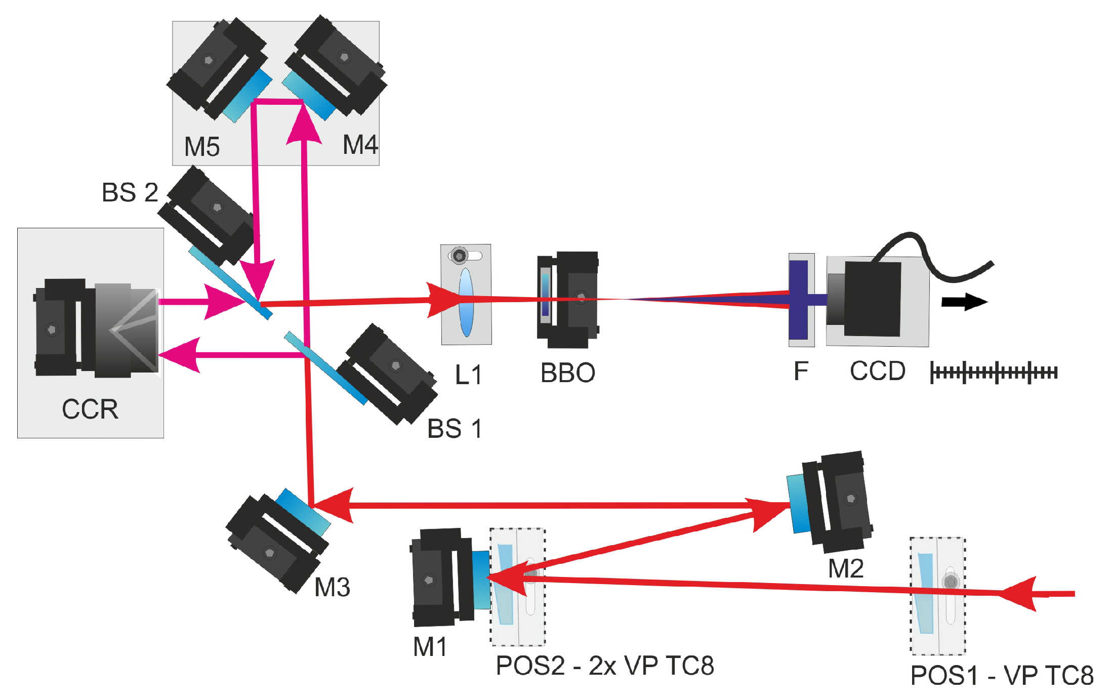
2. Experimental Scheme

The experimental setup is depicted in Figure 1. A femtosecond laser oscillator emitting sub-25-femtosecond pulses at a central wavelength of 800 nm (not shown in Figure 1) was used. A single vortex phase plate (VP) designed and fabricated to create optical vortices with topological charge |TC| = 8 was used. In this experiment, we used commercially available vortex phase plates (HoloOr). In these plates, the azimuthal change in their respective thickness, providing a phase change from 0 to 2$\pi$ for the desired wavelength, occurs in 16 discrete steps. Elements in which the thickness change is realized in 64 steps for the desired wavelength are also commercially available. In general, the larger number of steps with smaller height makes the vortex ring smoother in the azimuthal direction. In the context of the present analysis, where the azimuthal modulation is intentionally maximized, this is not significant but may be important in propagating optical vortex beams in nonlinear media.

To create an OV with |TC| = 8, the VP is positioned for a single pass of the beam (see POS1 in Figure 1). To produce an optical vortex with |TC| = 16, the same phase plate is used in a double-pass mode (see position POS2). For this purpose, it is set as close as possible in front of the flat mirror M1. (Please note that the same VP is used alternatively in one of the two positions, marked in Figure 1 by a dashed line.) The flat mirrors M2 and M3 are used to redirect the resulting singular beam to the interferometric part of the setup. Positions POS1 and POS2 of the vortex plates in front of the interferometer are not critical. The higher the encoded input topological charge, the larger the ring radius of the vortex beam. In this sense, real constraints are imposed by the apertures of the beam splitters BS1 and BS2 and of the lens L1. When tuning the vortex phase plate in position POS2, it is important that mirror M1 is as close as possible to (optimally in contact with) the vortex plate. Thus, on the return pass, the radius of the vortex ring is (practically) the same as after the first pass, and the doubled topological charge does not decay noticeably or symmetrically.

The used inverted-field interferometer involves beam splitters BS1 and BS2. The input beam is divided into two parts by BS1 and, after the corresponding number of reflections, the beams/pulses are overlapped in space and time on and after the beam splitter BS2. The optical vortex beams should be overlapped at the beam splitter BS2 at the output of the interferometer. The lengths of its two arms should be precisely equalized. These requirements, however, are typical for a femtosecond interferometer/autocorrelator and are relatively easy to fulfill. It is essential to note that in one of the interferometer arms, the beam experiences three reflections from the hollow corner-cube retroreflector CCR, while in the other arm it is reflected twice from the flat mirrors M4 and M5. As a result, one of the beams is flipped with respect to the other, motivating the classification of this interferometer as an inverted-field interferometer. The important consequence here is that the OVs appear at the second beam splitter with topological charges with opposite signs, but with equal absolute values of their TCs. The interference of these vortex beams leads to the generation of a multi-peaked necklace-like beam with azimuthal $\pi$-phase dislocations (see e.g., Figure 2 in [21]). The lens L1 focuses this singular beam slightly behind the 40 μm thick Beta-Barium Borate ($\beta -Ba{B}_2{O}_4$; BBO) nonlinear crystal to generate a second harmonic of the fundamental emission. The distance between lens L1 and the nonlinear crystal BBO is then determined by the requirement that the crystal be close to but in front of its focus. The simple reason for using such a thin nonlinear crystal is that it was available in our laboratory. It was used in a home-built second-order inverted-field femtosecond autocorrelator. We believe that the described technique can be applied with longer pulses and longer crystals. In this way, the efficiency in generating Bessel–Gaussian beams will improve. The only condition that needs to be kept is that the second harmonic must be generated first, and then it must pass through its focus (i.e., its Fourier transform in space must be performed afterwards). The generation of the second harmonic doubles the $\pi$-phase jumps in the input necklace beam to $2\pi$ in its second harmonic. In other words, azimuthal phase jumps are absent in the second harmonic of the ring-shaped multi-peaked necklace beam. This beam is not singular anymore and is only amplitude-modulated in the azimuthal direction. Since the focus of the lens L1 is aligned near to but after the nonlinear BBO crystal, the Fourier transform performed by it on the second-harmonic signal is on this ring-shaped beam with strongly pronounced azimuthal modulation. Passing only the second harmonic through the filter F, the CCD camera captures the generated Bessel–Gaussian beam in the second harmonic only.

The interferometer was not actively stabilized. It was aligned on a more or less standard 20 cm thick, vibration-isolated optical table. With 25-femtosecond pulses of 76 MHz repetition rate used, no noticeable negative influence of the weak fluctuations in the necklace contrast on the quality of the generated Bessel–Gaussian beams was observed. For the CCD camera used (CMOS-type, model Grasshopper 3, 2048 pix. × 2048 pix., pixel size 5.5 μm × 5.5 μm), the typical integration time was 0.3 s, which means an integration of about $2.3\times {10}^7$ pulses in time. Translating the CCD camera, we were able to follow the beam evolution at different phase propagation distances behind the focus of the lens.

3. Theoretical Model

3.1. General Remarks Regarding the Fourier Transformation of a Function in Polar Coordinates

Let us consider a function $f(r,\theta )$ depending on the polar coordinates $(r,\theta )$ in the following way

$$f(r,\theta )=\sum _{m=-\infty }^{\infty }{f}_m\left(r\right)e^{im\theta }.$$

(1)

Its two-dimensional Fourier transform $\tilde{f}(\rho .\psi )$ in polar coordinates $(\rho .\psi )$ is given by [22]

$$\tilde{f}(\rho .\psi )=\sum _m{i}^{-m}{e}^{im\psi }{h}_m\left(\rho \right)\left\{f_m\left(r\right)\right\}.$$

(2)

In the equation above, $h_m\left(\rho \right)\left\{f_m\left(r\right)\right\}$ denotes the Hankel transform of $f_m\left(r\right)$ and, as shown in [22],

$$h_m\left(\rho \right)\left\{f_m\left(r\right)\right\}={\int }_0^{\infty }{f}_m\left(r\right)J_m\left(\rho r\right)rdr.$$

(3)

Here, $J_m$ is the Bessel function of first kind and of order m. We are interested, however, in the much simpler case, in which the electric field amplitude has the form

$$E(r,\theta )=E_m\left(r\right)e^{im\theta }$$

(4)

and the integer m has the meaning of the topological charge of an OV. From the above formulae, it follows that the Fourier transform of the field $E(r,\theta )$ is

$$\tilde{E}(\rho ,\psi )=i^{-m}{e}^{im\psi }{\int }_0^{\infty }{E}_m\left(r\right)J_m\left(\rho r\right)rdr.$$

(5)

3.2. Analytical Model

Let us assume that the OV beams propagating in the two arms of the inverted-field interferometer (see Figure 1) are described by

$$E_{1m}(r,\theta )=E_{1m}\left(r\right)e^{im\theta }={\left({\displaystyle \frac{\sqrt{2}r}{r_0}}\right)}^{\left|m\right|}exp(-r^2/r_0^2)exp\left(im\theta \right),$$

(6)

$$E_{2m}(r,\theta )=E_{2m}\left(r\right)e^{-im\theta }={\left({\displaystyle \frac{\sqrt{2}r}{r_0}}\right)}^{\left|m\right|}exp(-r^2/r_0^2)exp(-im\theta ).$$

(7)

At this stage of the analysis, the number of reflections of the beams in the arms of the interferometer that differ by one is accounted for by the opposite signs of the TCs of the propagating optical vortex beams. After overlapping and passing them through a nonlinear crystal for second-harmonic generation (SHG), the second-harmonic (SH) field takes the form

$$E_{SHm}(r,\theta )\sim {[E_{1m}(r,\theta )+E_{2m}(r,\theta )]}^2=E_{1m}^2(r,\theta )+E_{2m}^2(r,\theta )+2E_{1m}(r,\theta )E_{2m}(r,\theta ).$$

(8)

As mentioned when introducing the experimental scheme in Figure 1, we align the focusing lens before the SH crystal so as to position its back focal plane right after the crystal. The thin lens is performing a Fourier transformation (FT) in space. Analytically, the resulting electric field in this focal plane (i.e., in the artificial far field) is given by

$${\tilde{E}}_{SHm}(\rho ,\psi )=FT\left\{E_{SHm}(r,\theta )\right\}={\tilde{E}}_{SH1m}(\rho ,\psi )+{\tilde{E}}_{SH2m}(\rho ,\psi )+{\tilde{E}}_{SH12m}(\rho ,\psi ).$$

(9)

As already mentioned, the FT is represented by a Hankel transform. The corresponding analytical expressions for the first two field components in Equation (9) are

$${\tilde{E}}_{SH1m}(\rho ,\psi )=i^{-2m}{e}^{i2m\psi }{h}_{2m}\left(\rho \right)\left\{E_{1m}^2\left(r\right)\right\},$$

(10)

$$\begin{array}{cc}\hfill {\tilde{E}}_{SH2m}(\rho ,\psi )=& i^{2m}{e}^{-i2m\psi }{h}_{-2m}\left(\rho \right)\left\{E_{2m}^2\left(r\right)\right\}=i^{2m}{e}^{-i2m\psi }{(-1)}^m{h}_{2m}\left(\rho \right)\left\{E_{2m}^2\left(r\right)\right\}=\hfill \\ \hfill & i^{-2m}{e}^{-i2m\psi }{h}_{2m}\left(\rho \right)\left\{E_{2m}^2\left(r\right)\right\},\hfill \end{array}$$

(11)

where

$$J_{-m}\left(x\right)={(-1)}^m{J}_m\left(x\right),$$

(12)

(see, e.g., [23]), while the last third term of Equation (9) is simplified to

$${\tilde{E}}_{SH12m}(\rho ,\psi )=h_0\left\{E_{1m}\left(r\right)E_{2m}\left(r\right)\right\}.$$

(13)

Finally, we are ready to calculate the intensity distribution of the SH signal in the artificial far field:

$$\begin{array}{cc}\hfill I_m(\rho ,\psi )=& |{\tilde{E}}_{SHm}{(\rho ,\psi )|}^2=\hfill \\ \hfill & 4^{-(3m+1)}{r}_0^4{e}^{-r_0^2{\rho }^2/4}\left({64}^m{\Gamma }^2(m+1)L_m^2\left(r_0^2{\rho }^2/8\right)+{\left(r_0\rho \right)}^{4m}{sin}^2\left(2m\psi \right)\right).\hfill \end{array}$$

(14)

According to [24], the Laguerre function $L_m$ can be substituted with Bessel function (see Equation (3) in [24]).

$$\begin{array}{cc}\hfill I_m(\rho ,\psi )=& 4^{-(3m+1)}{r}_0^4{e}^{-r_0^2{\rho }^2/4}\left(4^{6m}{e}^{r_0^2{\rho }^2/8}{(m!)}^4{J}_0^2\left((r_0\rho /2)\sqrt{1+2m}\right)+{\left(r_0\rho \right)}^{4m}{sin}^2\left(2m\psi \right)\right).\hfill \end{array}$$

(15)

This is the desired analytical result. It is valid if the polynomial order $m\gg 1$. In our case, m = 8, playing the role of the initial topological charge to be subsequently erased, nearly fulfills this condition, and m = 16 satisfies the condition unambiguously. An additional proof for the validity of this substitution is that Equation (14) compared to the Bessel–Gaussian approximation Equation (15) yields reduced ${\chi }^2=5.7\times {10}^{-5}$ and adjusted $R^2$ = 0.993. The multi-peaked necklace beam with azimuthal $\pi$-phase jumps, having undergone second-harmonic generation and no longer carrying phase dislocations, is expected to generate an on-axis Bessel–Gaussian beam and a diffuse divergent background signal. Figure 2 is intended to support this statement. In Figure 2a, we plot the SH signal given by Equation (14) for TC $m=16$, $r_0=0.5$, $\rho =\sqrt{x^2+y^2}$, $\psi =arctan(y/x)$, and $(x,y)\in [-30,30]$. The created BGB (its central peak and four surrounding rings) are clearly seen. For better visibility, nearly 10% of the bottom right quarter of this frame is adjusted in brightness and contrast. In this sector, one can recognize the weak diffuse halo as well, which results from the last term in Equation (14). In Figure 2b, using the same parameters, we plot the SH intensity given by Equation (15). The only difference between panels (b) and (a) is that the mentioned halo is barely visible anymore, despite the fact that the term describing it is present in Equation (15) as well.

The analytical results above are valid for cw beams; however, outside laser cavities, the SH is usually generated with pulsed beams (in the case described below, with femtosecond pulses). Because of this, however for simplicity, we assumed Gaussian shapes of the input pulses of duration $t_0$ and introduced a possible time delay $\tau$ between them. In this way, similarly to Equations (6) and (7), the OV beams/pulses propagating in the two arms of the inverted-field interferometer (see Figure 1) are described by

$$E_{1m}(r,\theta ,t)=E_{1m}\left(r\right)e^{im\theta }exp(-t^2/t_0^2)e^{i{\omega }_{0}t},$$

(16)

$$E_{2m}(r,\theta ,t)=E_{2m}\left(r\right)e^{-im\theta }exp(-{(t-\tau )}^2/t_0^2)e^{i{\omega }_0(t-\tau )}.$$

(17)

Following the described procedure, performing a final integration in time (in order to simulate the action of a slow photodetector), we arrive at the generalized result

$$\begin{array}{cc}\hfill I_m(\rho ,& \psi ,\tau )=I_0\left(I_1\left(exp({\tau }^2/\left(2t_0^2\right))-cos(4m\psi +{\omega }_0\tau )\right)+2^{(6m+1)}{(m!)}^2{L}_m^2(r_0^2{\rho }^2/8)\right)\approx \hfill \\ \hfill & I_0\left(I_1\left(exp({\tau }^2/\left(2t_0^2\right))-cos(4m\psi +{\omega }_0\tau )\right)+2^{(6m+1)}{(m!)}^2{J}_0^2\left((r_0\rho /2)\sqrt{1+2m}\right)\right),\hfill \end{array}$$

(18)

where $I_0=4^{-(3m+2)}\sqrt{\pi }{r}_0^4{t}_{0}exp(-r_0^2{\rho }^2/4)exp(-{\tau }^2/t_0^2)$ and $I_1=\sqrt{2}exp(({\tau }^2/\left(2t_0^2\right)){\left(r_0\rho \right)}^{4m}$ are introduced to simplify the notations. For perfectly synchronized pulses (i.e., for $\tau$ = 0), it reproduces Equation (15) with a normalization coefficient.

4. Results and Discussion

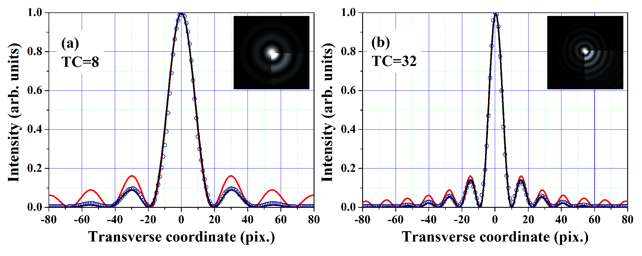
4.1. Data from the Analytical Model

In Figure 3, using the derived analytical results, we graphically illustrate the physics of the creation of necklace beams, their second-harmonic generation, and subsequent conversion to Bessel–Gaussian beams. In panels (a1) and (a2), we show the intensity and phase profiles of an input vortex beam with TC = 8. Since a single vortex plate with TC = 8 was used, in the experiment, this VP was located in position POS1 (see Figure 1). The OVs in our experiment were generated directly in the beams/pulses of a sub-25-femtosecond Ti:Sapphire mode-locked laser. The vortex ring in panel (a1) of Figure 3 is smooth. Experimentally, it can be observed (see Figure 1) between the second beam splitter BS2 and the focusing lens L whether one of the interferometer arms is blocked or whether the time delay between the pulses is larger than their durations. The phase profile in panel (a2) clearly demonstrates eight sawtooth-like sectors in which the phase linearly increases from $-\pi$ to $+\pi$. As expected, the intensity distribution of the SH signal (panel (a3)) is also ring-shaped, with a decreased ring width in the radial direction, and its topological charge is doubled (see panel (a4)).

When the OVs with equal absolute values but with opposite signs of their TCs interfere at and after BS2 (see Figure 1), a necklace beam is formed as shown in panels (b1) and (c1). The number of petals of the multi-peaked structure is twice the absolute value of the respective TC. The used gray scale for presenting the phase profiles shows that gray and black correspond to phases zero and $-\pi$, respectively. Therefore, each two peaks of each of the necklace structures in panels (b1) and (c1) are separated by azimuthal $\pi$-phase dislocations (see panels (b2) and (c2)). Neither the necklace beams nor the SH beams carry spiral phase dislocations of OVs anymore. Although input OVs with topological charges 8 and 16 are used in the experiment discussed below, here we prefer to present the cases for |TC|=8 and 32 because the effects on the generated Bessel–Gaussian beams are more pronounced for higher TCs.

Let us focus our attention on the phase profiles (b4) and (c4) of the beams after the SH generation process. The azimuthal $\pi$-phase dislocations are doubled. This can be demonstrated by the fact that in the azimuthal direction, the phase either does not change or changes from $-\pi$ to $+\pi$ (from black to white or vice versa). Effectively, azimuthal phase modulations do not exist and do not lead to modulation of the rings of the resulting Bessel–Gaussian beams (see panels (b3) and (c3)). On the other hand, the phase between each two rings changes with $\pi$ in radial direction (from black/white to gray or vice versa; see the color scale). This is the reason for the maximal modulation depth between the rings of the BGBs and is their known characteristic [3]. The Bessel–Gaussian beams can be recognized in panels (b3) and (c3) by the dominating central peaks surrounded by concentric rings with amplitudes decreasing in the radial direction. There is also a well-pronounced tendency that the higher the TC of the input OV beam, the narrower the central peak and the more visible its satellite rings (see also, e.g., Figure 8 in [10]).

In Figure 4a, with blue open circles, we show the transverse cross-section of a BGB calculated using Equation (15) for TC = 8. It is intentionally shifted by 0.1 arbitrary units from the analytical squared Bessel function (red solid curve) with infinite satellite radial peaks (not clearly seen here). For comparison, the calculated squared Bessel–Gaussian diametral distribution (black solid curve) shows equally good agreement in the radial positions with the satellite peaks of the numerical profile (hollow blue circles). However, due to the Gaussian envelope, the intensities of the satellite rings decrease visibly faster. This is the situation in real experiments, which can only be performed with laser beams of finite dimensions. The insets show the calculated intensity distributions of the BGBs from which the diametral cross-sections (open circles) are extracted. For better visibility, one quarter of each of them are adjusted in brightness and contrast. In Figure 4b, following the same style of notation, we show the calculated results for TC = 32 and the corresponding approximating curves. Again, a very good match of the satellite ring positions (here, the satellite peaks) as well as the maximal depth of intensity modulation between them can be seen. It is also clearly visible that the higher the TC of the input OV beam, the narrower the central peak and the more visible its satellite rings.

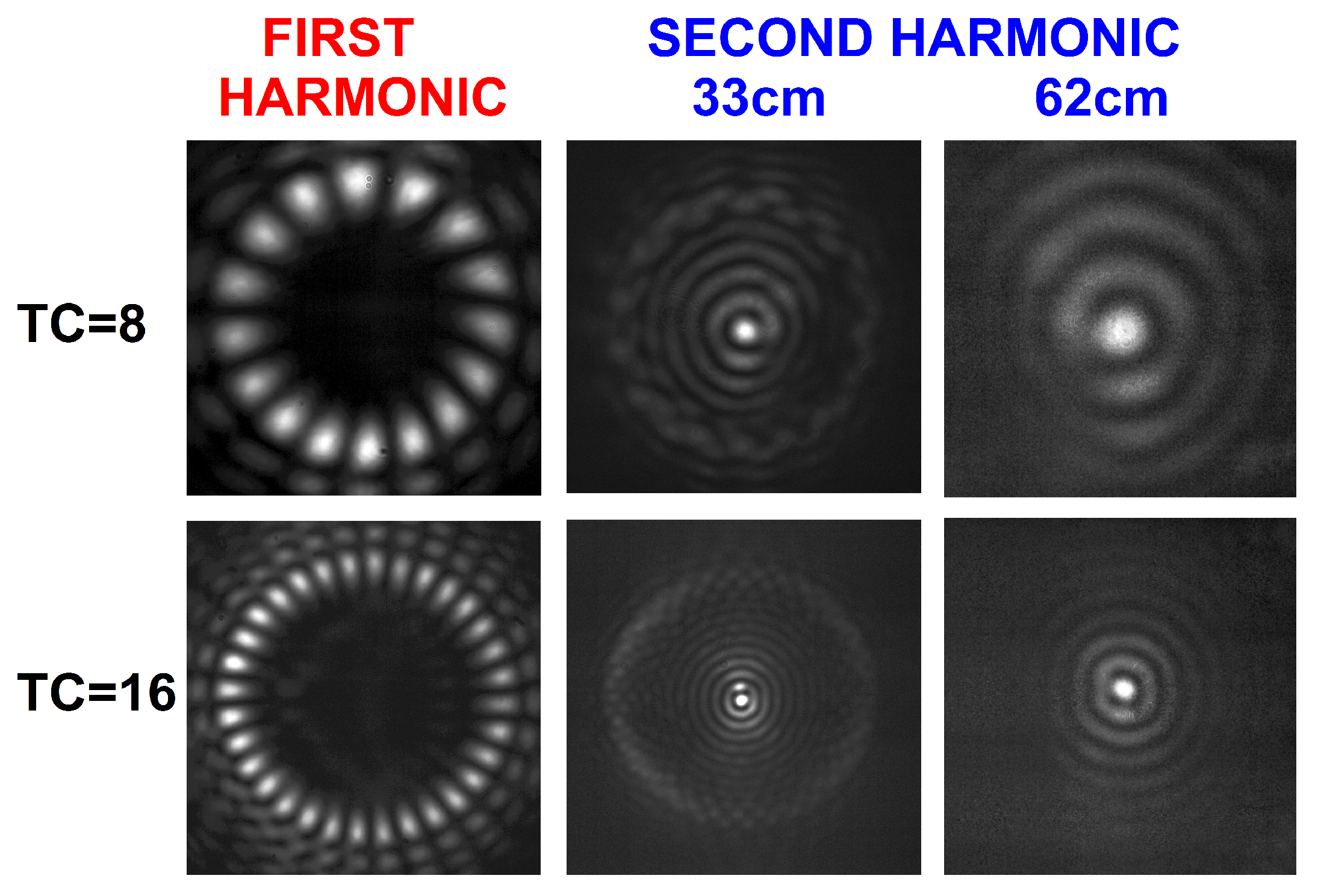
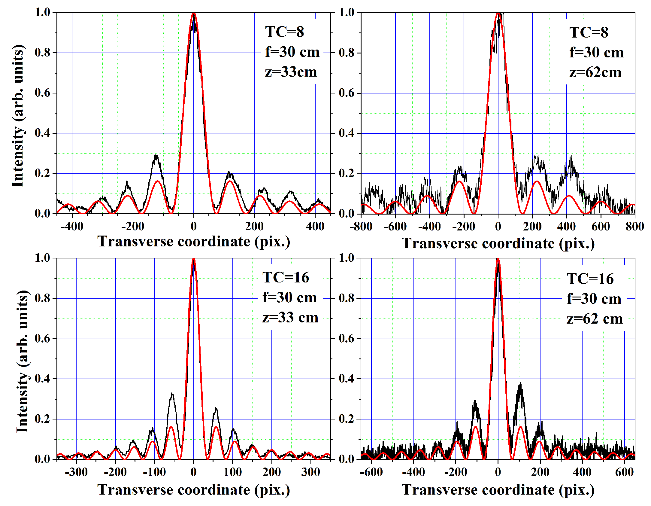
4.2. Experimental Results and Discussion

The same vortex phase plate, designed and fabricated to generate OVs with topological charges TC = 8 at a wavelength of 800 nm, was used in the experiments. Indeed, when the laser beams/pulses passed through it once (with no propagation in an interferometer), OVs with smooth vortex rings with no axial modulation were generated. When the laser beams/pulses passed through it twice, OVs with TC = 16 were generated, also without noticeable modulation but, as expected, with a larger ring radius. Regarding the situation on and after the second beam splitter of the interferometer (see Figure 1), when one of these pulsed beams entered the inverted-field interferometer, the corresponding necklace structure shown in the left column of frames in Figure 5 was observed. The beams no longer carried point phase dislocations but azimuthal $\pi$-phase dislocations (see also frames (b2) and (c2) in Figure 3). As a consequence, in the first harmonic beams, the rings were strongly azimuthally modulated. In this case, the CCD camera was positioned in front of the NL crystal. As expected, the accumulated diffraction caused outer-lying oscillations of the necklace. The beam propagated further to the nonlinear crystal in which its second harmonic was generated. In the SH, the $\pi$-phase jumps were absent. Insofar as the focus of the lens was close to but behind the crystal, the lens performed a Fourier transform of the harmonic signal in space. The generated Bessel–Gaussian beams at input TCs = 8 and 16 are shown at a propagation lengths of 33 cm (Figure 5, middle column of frames) and at 62 cm (Figure 5, right column of frames). It can be seen that the higher the TC of the input beam, the narrower the central peak of the GBB. At a propagation distance of 33 cm, a structured halo is visible on the outer side of the satellite rings. It has a high transverse velocity, rapidly separates from the BGBs, and is no longer visible at 62 cm propagation distance. Apparently, within this 30 cm beam propagation, the central peaks, even weakly expressed, undergo diffraction. We will return to its quantification later. It is now appropriate to say that the present experiment carried out with a quartz phase plate with an encoded TC = 8 in a double-pass configuration is almost at the lower limit of the applicability of the method [10]. With an OV phase plate with TC∼32 and higher, substantially lower values and a quasi-nondiffracting mode of propagation can be reached [10].

In Figure 6, we show cross-sections of the experimentally recorded BGB profiles in the generated second harmonic shown in Figure 5. The black and somewhat noisy curves present the experimental data, while the red curves show the respective approximations by squared Bessel functions. The reason for the increase in the noise as the propagation length increases (see the right graphs in Figure 6) is the relatively weak Bessel–Gaussian beam signal in the second harmonic of the pump. This relatively weak signal is due to both the thin nonlinear crystal used and to the need to keep the focus of the lens behind the this crystal, thus lowering the intensity of the pump wave in the crystal. For the lower TC = 8 and for propagation distance z = 33 cm, the precision of the approximation of the experimental data is characterized by ${\chi }^2=8.8\times {10}^{-4}$ and $R^2$ = 0.978, which at 62 cm decreases to ${\chi }^2=3.5\times {10}^{-3}$ and $R^2$ = 0.92. For TC = 16 and at z = 33 cm, ${\chi }^2=1.3\times {10}^{-3}$ and $R^2$ = 0.956, whereas at z = 62 cm, ${\chi }^2=2.3\times {10}^{-3}$ and $R^2$ = 0.915. It is worth noting that the abscissae of the plots are different. Comparing the left two graphs only, it is clearly seen that at 33 cm, after the lens focus, the scale of the graph for TC = 8 is wider than that for TC = 16. Moreover, the central peak of the BGB for TC = 8 is visibly wider than this for TC = 16. The same is clearly expressed when comparing the right plots for propagation lengths 62 cm after lens focus. The second aspect we would like to note is the good agreement between the positions of the peaks of the satellite rings. Unfortunately, the contrast between the central peak and its satellites is visibly higher in the approximating curves compared to the experimental ones. It can also be seen that the higher divergence of the central peak of the BGB for TC = 8 at the same propagation length of 62 cm leads to a faster signal decay of the second harmonic and to higher noise compared to the TC = 16 case.

At this stage, considering the data shown in Figure 5 and Figure 6, it can be concluded that the generation of BGBs in the second harmonic of necklace beams is successful, even at the relatively low topological charges of the used input vortex beams. In order to evaluate the accuracies in determining the divergences in the different cases, we first evaluated the standard errors in determining the widths of the central peaks of the BGBs and the accuracy in measuring the propagation length. Typically, as in the particular case of TC = 16 and f = 30 cm, the standard errors in determining the peak width we accounted for are 0.2% at 33 cm, 0.4% at 62 cm, 0.6% at 82 cm, and 0.8% at 120 cm, and the overall (slightly pessimistic) standard error was estimated to be 2.4%. The obtained data for the divergences of the central peaks are as follows:

      for TC = 8 and f = 12.5 cm—divergence 1.2 (±0.1) mrad

           for f = 30 cm—divergence 500 (±22) μrad

      for TC = 16 and f = 30 cm—divergence 243 (±6) μrad

           for f = 50 cm—divergence 180 (±4) μrad.

The reasonable expectation based on our previous studies is that the divergences can be further reduced by using vortex phase plates with encoded higher TCs (see, e.g., [10]). An overview of the achievements of other groups in lowering the divergences of Bessel–Gaussian beams (also referred to in the literature as structured laser beams) shows data in the wide range from 450 μrad [25] to 10 μrad [26] and even down to 4 μrad [9]. Using the method applied also here, under unperturbed initial conditions, we produced in our laboratory BGBs with divergences of 45 μrad [12]. In this sense, the 180 μrad divergence reported here, under intentionally strongly modulated initial conditions and using lenses with relatively short focal length, has the potential for improvement but fits well into the state-of-the-art results on the problem.

Generally speaking, with all starting conditions unchanged, lower divergences are obtained with lenses of longer focal lengths. In the experiments, we used three different lenses to emphasize that the difference in the focal lengths is not critical. In all three cases, the requirement that their foci should be after the nonlinear crystal generating the second harmonic was kept. In other words, the Fourier transform in space took place after the frequency doubling process of the necklace beam was completed. But different focal lengths mean different intensities of the pump beam in the BBO crystal, and thus a different energy density detected by the CCD camera at a fixed position. This is the reason why at longer distances, with lenses with longer focal lengths, the signal-to-noise ratio is lower. An improvement of the situation could be obtained with a thicker nonlinear crystal. It might be desirable to use input optical vortices with higher topological charges to finally obtain Bessel–Gaussian beams with narrower central peaks. In the plane of the lens, however, the necklace beam will have a larger radius, and its lower intensity in the nonlinear medium will lower the signal level of the second harmonic. This could, to some extent, be compensated for by using a shorter focal length of the focusing lens, unfortunately at the cost of a higher beam divergence.

Perhaps a final remark is appropriate here. Probably the first generation of BGBs from necklace beams were revealed in our previously published work [21] devoted to a new femtosecond pulse measurement technique (see Figure 6b in [21]) but were explored in detail (successfully analytically modeled and experimentally investigated) in this study.

5. Conclusions

In this paper, we present experimental evidence confirmed by analytical results that Bessel–Gaussian beams can be generated in femtosecond pulsed laser fields by generating the second harmonic of ring-shaped, strongly azimuthally modulated necklace beams and their subsequent Fourier transformation in space. The necklace beams are created by the interference of optical vortex beams carrying point phase dislocations. The role of second-harmonic generation is to remove the azimuthal phase dislocations in the necklace beams. The Fourier transform in space is performed by focusing these second-harmonic beams in thin lenses. For an input beam with a topological charge of 16, divergence of the central peak of the BGB down to 180 μrad was measured. Further lowering of this divergence can be achieved with input beams of higher topological charges. The energy efficiency of the process could be increased by using thicker nonlinear crystals.

References

1. Durnin, J. Exact solutions for nondiffracting beams. I. The scalar theory. J. Opt. Soc. Am. A 1987, 4, 651–654. [Google Scholar] [CrossRef]
2. Khonina, S.N.; Ustinov, A.V.; Chávez-Cerda, S. Generalized parabolic nondiffracting beams of two orders. J. Opt. Soc. Am. A 2018, 35, 1511–1517. [Google Scholar] [CrossRef]
3. Lin, Y.; Seka, W.; Eberly, J.H.; Huang, H.; Brown, D.L. Experimental investigation of Bessel beam characteristics. Appl. Opt. 1992, 31, 2708–2713. [Google Scholar] [CrossRef]
4. McGloin, D.; Dholakia, K. Bessel beams: Diffraction in a new light. Contemp. Phys. 2005, 46, 15–28. [Google Scholar] [CrossRef]
5. Durnin, J.; Miceli, J.J.; Eberly, J.H. Diffraction-free beams. Phys. Rev. Lett. 1987, 58, 1499–1501. [Google Scholar] [CrossRef]
6. Yu, X.; Todi, A.; Tang, H. Bessel beam generation using a segmented deformable mirror. Appl. Opt. 2018, 57, 4677–4682. [Google Scholar] [CrossRef]
7. Bowman, R.; Muller, N.; Zambrana-Puyalto, X.; Jedrkiewicz, O.; Trapani, P.D.; Padgett, M.J. Efficient generation of Bessel beam arrays by means of an SLM. Eur. Phys. J. Spec. Top. 2011, 199, 159–166. [Google Scholar] [CrossRef]
8. Duocastella, M.; Arnold, C. Bessel and annular beams for materials processing. Laser Photonics Rev. 2012, 6, 607–621. [Google Scholar] [CrossRef]
9. Vetter, C.; Steinkopf, R.; Bergner, K.; Ornigotti, M.; Nolte, S.; Gross, H.; Szameit, A. Realization of Free-Space Long-Distance Self-Healing Bessel Beams. Laser Photonics Rev. 2019, 13, 1900103. [Google Scholar] [CrossRef]
10. Stoyanov, L.; Zhekova, M.; Stefanov, A.; Stefanov, I.; Paulus, G.G.; Dreischuh, A. Zeroth- and first-order long range non-diffracting Gauss-Bessel beams generated by annihilating multiple-charged optical vortices. Sci. Rep. 2020, 10, 21981. [Google Scholar] [CrossRef]
11. Stoyanov, L.; Zhang, Y.; Dreischuh, A.; Paulus, G.G. Long-range quasi-non-diffracting Gauss-Bessel beams in a few-cycle laser field. Opt. Express 2021, 29, 10997–11008. [Google Scholar] [CrossRef]
12. Stoyanov, L.; Topuzoski, S.; Paulus, G.G.; Dreischuh, A. Optical vortices in brief: Introduction for experimentalists. Eur. Phys. J. Plus 2023, 138, 702. [Google Scholar] [CrossRef]
13. Berry, M.V. Making waves in physics. Nature 2000, 403, 21. [Google Scholar] [CrossRef]
14. Heckenberg, N.R.; McDuff, R.; Smith, C.P.; White, A.G. Generation of optical phase singularities by computer-generated holograms. Opt. Lett. 1992, 17, 221–223. [Google Scholar] [CrossRef]
15. Swartzlander, G.A.; Law, C.T. Optical vortex solitons observed in Kerr nonlinear media. Phys. Rev. Lett. 1992, 69, 2503–2506. [Google Scholar] [CrossRef]
16. Beijersbergen, M.; Coerwinkel, R.; Kristensen, M.; Woerdman, J. Helical-wavefront laser beams produced with a spiral phaseplate. Opt. Commun. 1994, 112, 321–327. [Google Scholar] [CrossRef]
17. Lee, W.H. Computer-Generated Holograms: Techniques and Applications. In Progress in Optics; Wolf, E., Ed.; Elsevier: Amsterdam, The Netherlands, 1978; Volume 16, pp. 119–232. [Google Scholar] [CrossRef]
18. Allen, L.; Beijersbergen, M.W.; Spreeuw, R.J.C.; Woerdman, J.P. Orbital angular momentum of light and the transformation of Laguerre-Gaussian laser modes. Phys. Rev. A 1992, 45, 8185–8189. [Google Scholar] [CrossRef]
19. Yu, P.; Chen, S.; Li, J.; Cheng, H.; Li, Z.; Liu, W.; Xie, B.; Liu, Z.; Tian, J. Generation of vector beams with arbitrary spatial variation of phase and linear polarization using plasmonic metasurfaces. Opt. Lett. 2015, 40, 3229–3232. [Google Scholar] [CrossRef]
20. Li, J.S.; Chen, J.Z. Multi-beam and multi-mode orbital angular momentum by utilizing a single metasurface. Opt. Express 2021, 29, 27332–27339. [Google Scholar] [CrossRef]
21. Dimitrov, N.; Zhekova, M.; Zhang, Y.; Paulus, G.G.; Dreischuh, A. Background-free femtosecond autocorrelation in collinearly-aligned inverted field geometry using optical vortices. Opt. Commun. 2022, 504, 127493. [Google Scholar] [CrossRef]
22. Piessens, R. The Hankel Transform. The Transforms and Applications Handbook, 2nd ed.; CRC Press LLC: Boca Raton, FL, USA, 2000. [Google Scholar]
23. Abramovitz, M.; Stegun, I.A. Handbook of Mathematical Functions with. Formulas, Graphs, and Mathematical Tables. Appl. Math. Seties 1972, 55, 358. [Google Scholar]
24. Sheppard, C.J.R.; Porras, M.A. Comparison between the propagation properties of Bessel–Gauss and generalized Laguerre–Gauss beams. Photonics 2023, 10, 1011. [Google Scholar] [CrossRef]
25. Tissandier, F.; Sebban, S.; Ribière, M.; Gautier, J.; Zeitoun, P.; Lambert, G.; Goddet, J.P.; Burgy, F.; Valentin, C.; Rousse, A.; et al. Bessel spatial profile of a soft x-ray laser beam. Appl. Phys. Lett. 2010, 97, 231106. [Google Scholar] [CrossRef]
26. Sulc, M.; Gayde, J.-C. Low Divergence Structured Beam In View Of Precise Long-Range Alignment. EPJ Web Conf. 2022, 266, 10024. [Google Scholar] [CrossRef]
Figure 1. Experimental setup. POS1 and POS2—alternative positions, at which the vortex phase plate VP fabricated to produce optical vortices with topological charge |TC| = 8 is located. M1–M5—flat, silver-coated mirrors. BS1, BS2—beam splitters. CCR—hollow corner-cube retroreflector. L1—fused silica lens (f = 12.5 cm, 30 cm, or 50 cm). BBO—40 μm thick Beta-Barium Borate crystal. F—interference filter for transmitting around 400 nm. CCD—charge-coupled device camera mounted on a translation stage.
Photonics 12 00119 g001
Figure 2. Visualization of the exact result given by Equation (14) (frame (a)) and of the approximation given by Equation (15) (frame (b)). For better visibility, ∼10% of each frame is adjusted, in the same manner, in brightness and saturation. The only visible difference is the presence (frame (a))/absence (frame (b)) of the weak halo outside the satellite rings. Parameters: TC m = 16 , r 0 = 0.5 , ρ = x 2 + y 2 , ψ = arctan ( y / x ) , where ( x , y ) [ 30 , 30 ] .
Photonics 12 00119 g002
Figure 3. Numerical results. Intensity (a1) and phase portraits (a2) of an OV with TC = 8 in the pump wave, and the respective intensity (a3) and phase profiles (a4) of the SH wave. Intensity distributions of the necklace beams for TC = 8 (b1) and 32 (c1) and their phases (b2,c2), respectively, in front of the Fourier transforming lens (see Figure 1). (b3,c3)—Intensity distributions of the Bessel–Gaussian beams in the SH wave and their phase portraits ((b4) and (c4), respectively). See the text for details.
Photonics 12 00119 g003
Figure 4. Numerical results. Hollow blue circles—cross-sections of BGBs generated numerically (Equation (15)) using input OVs with TCs = 8 (graph (a)) and 32 (graph (b)). Red solid curves—pure squared Bessel functions. Black solid curves—squared Bessel–Gaussian functions whose finite number of satellite peaks decay faster in the radial direction. Insets—calculated intensity distributions of the BGBs from which the diametral cross-sections (open circles) are extracted. The cross-sections of the numerically generated BGBs (hollow blue circles) compared to the respective Bessel–Gaussian fits (solid black curves) yield reduced χ 2 = 5.6 × 10 5 and adjusted R 2 = 0.997 for TC = 8, χ 2 = 7.3 × 10 5 and R 2 = 0.993 for TC = 32.
Photonics 12 00119 g004
Figure 5. Experimental results. (Left) frames—necklace beams generated with OVs with TCs = 8 and 16, as recorded in front of the Fourier transforming focusing lens L (f = 30 cm; see Figure 1). (Middle) and (Right) columns—energy density distributions of Bessel–Gaussian beams recorded 33 cm and 62 cm behind the BBO crystal for SH generation.
Photonics 12 00119 g005
Figure 6. Experimental results. Black curves—cross-sections of the Bessel–Gaussian beams shown in the middle and right columns in Figure 5 for TC = 8 ((top) two graphs) and TC = 16 ((bottom) graphs) measured 33 cm and 62 cm behind the focus of the Fourier-transforming lens (f = 30 cm). Red curves—respective approximations with squared Bessel functions.
Photonics 12 00119 g006
Disclaimer/Publisher’s Note: The statements, opinions and data contained in all publications are solely those of the individual author(s) and contributor(s) and not of MDPI and/or the editor(s). MDPI and/or the editor(s) disclaim responsibility for any injury to people or property resulting from any ideas, methods, instructions or products referred to in the content.