Article

Channel Characterization and Comparison in Industrial Scenario from Sub-6 GHz to Visible Light Bands for 6G

1
State Key Laboratory of Networking and Switching Technology, Beijing University of Posts and Telecommunications, Beijing 100876, China
2
State Key Laboratory of Information Photonics and Optical Communications, Beijing University of Posts and Telecommunications, Beijing 100876, China
3
China Mobile Research Institute, Beijing 100053, China
*
Author to whom correspondence should be addressed.
Photonics 2025, 12(3), 257; https://doi.org/10.3390/photonics12030257
Submission received: 24 January 2025 / Revised: 3 March 2025 / Accepted: 3 March 2025 / Published: 13 March 2025
(This article belongs to the Special Issue Advanced Technologies in Optical Wireless Communications)

Abstract

:
The industrial scenario is indispensable for ubiquitous 6G coverage, which demands hyper-reliable and low-latency communication for full automation, control, and operation. To meet these demands, it is widely believed that it is necessary to introduce not only the conventional sub-6 GHz bands but also high-frequency technologies, such as millimeter wave (mmWave), terahertz (THz), and visible light bands. In this paper, we conduct a channel characterization and comparison in the industrial scenario from the sub-6 GHz to visible light bands. The channel characteristics, including the path loss (PL), root mean square (RMS) delay spread (DS), and angle spread (AS), were analyzed with respect to the frequency dependence and the distance dependence. On the one hand, the visible light band exhibited significant differences in channel characteristics compared to the electronic wave band. Due to the line-of-sight transmission of VLC, the visible light band had a higher path loss, and the path loss exponent reached 3.84. Due to the Lambertian radiation pattern, which has a wide range of reflection angles, the AS of the visible light band was much larger than that of the electronic wave band, which were 1.73 and 0.80 for the visible light and THz bands, respectively. On the other hand, the blockage effect of the metal instruments in the industrial scenario will greatly affect the channel characteristics. As the transceiver distance grows large, signals from both sides of the receiver will be blocked by metal instruments, resulting in a decreasing trend in the RMS DS for the electronic wave band. Moreover, the statistical characteristics of the channel properties were modeled and compared with the 3GPP TR 38.901 standard. It was found that the height of the receiver caused the difference between the proposed model and the 3GPP model and needs to be taken into account when modeling. Furthermore, we extended the 3GPP model to the THz and VLC bands and provided the statistical parameters of the channel characteristics for all frequency bands. This study can provide insights for the evaluation and standardization of multi-frequency communication technology in the industrial scenario.

1. Introduction

At the recent International Telecommunication Union Radiocommunication (ITU-R) Working Party (WP) 5D meeting, a new recommendation was approved which highlights six usage scenarios of IMT-2030 [1]. As a typical usage case of the hyper-reliable and low-latency communication scenario, the industrial scenario has received widespread attention again. It extends the Ultra-Reliable and Low-Latency Communication (URLLC) of IMT-2020 and covers specialized use cases that are expected to have more stringent requirements for enhanced reliability, low latency, and precise positioning [2].
To satisfy the high performance metrics of IMT-2030 for the industrial scenario, communication technology continues to develop from sub-6 GHz toward high-frequency bands [3]. Firstly, sub-6 GHz bands have low propagation loss and a strong coverage capability which can provide extensive coverage for the industrial scenario, which has a larger physical size than an ordinary indoor scenario [4]. Secondly, to meet the typical business requirements of an ultra-wide bandwidth and ultra-low-latency transmission in the industrial scenario, high-frequency communication technologies such as millimeter wave (mmWave) and terahertz (THz) bands are applied [5]. Thirdly, excessive electromagnetic interference will be generated due to the operation of the abundant equipment in the industrial scenario, and the visible light band is regarded as a solution to interference problems due to the significant frequency isolation between the light and radio waves. Furthermore, an abundance of metallic scatterers in the industrial scenario produces specular reflection which results in an increasing intensity of reflection and dense multipath components (MPCs) [6]. Due to the different capabilities for the reflection, diffraction, and scattering of signals in different frequency bands, the impact of the frequency is more pronounced than in traditional indoor hotspot scenarios. Hence, it is imperative to explore the propagation characteristics for all frequency bands within an industrial scenario and elucidate the distinct channel properties across various frequency bands.

1.1. Literature Review

Looking at the existing literature, a number of works have been reported on channel characteristics and modeling at multiple bands in the industrial scenario, as shown in Table 1. In the following subsection, we will review the progress of industrial scenario channels according to frequency bands.
With respect to the sub-6 GHz band, the existing channel research on the industrial scenario mainly concentrates on the path loss and root mean square (RMS) delay spread (DS), and the reference distance (CI) model is mainly used for path loss modeling. In [7], the author investigated the multi-wall–multi-floor (MWF) model of the industrial environment, and measurements were conducted at 2.4 GHz in the multistoried building. By comparing the MWF model with the path loss obtained through measurements, it was found that the MMF model can accurately characterize the path loss in industrial scenarios. In [8], the author presented channel measurements at 4.145 GHz in both a sparse industrial environment with a normal size and a dense industrial environment with an extra-large size. It was found that the line-of-sight (LOS) path loss exponents (PLEs) of the CI model were 1.24 and 1.5, and the RMS DS was 22 and 83.2 for the sparse environment and dense environment, respectively. This indicates that the path loss and RMS DS are dependent on the industrial environment. In [9], the CI path loss model and the RMS DS were investigated at 4.1 GHz in both LOS and non-line-of-sight (NLOS) scenarios. The PLEs for the LOS and NLOS cases were 1.96 and 2.72, and the majority of the RMS DSs for the LoS and NLoS cases were 172 ns and 204 ns, respectively. However, due to the lack of detailed descriptions of the measurement scenario and measurement setting in [9], it is difficult to explain why there were significant differences in the channel characteristic parameters between [8,9]. Moreover, research on the spatial domain is still lacking.
Regarding the mmWave band, channel research for the industrial scenario mainly focuses on 28 GHz [6,10,11,12] and 142 GHz [14,15,16], which is also known as the sub-THz frequency band. There is sufficient research on channel characteristics such as the path loss, RMS DS, and angle spread (AS), and many influencing factors, such as the antenna height, antenna polarization configurations, and time-varying effects, have been taken into account. In [6], the path loss, DS, and AS were analyzed and modeled in a factory-like scenario at 28 GHz. The path loss was modeled by both the CI model and the floating intercept (FI) model, and the FI model showed high accuracy. Moreover, the RMS DS and AS were modeled by a linear function, and the cumulative distribution function (CDF) fitting line as well as the fitting parameters were given. Furthermore, it was found that the antenna heights would have an impact on these channel characteristics. In [10], a ray-tracing-based simulation was conducted at 28 GHz in a light factory and a heavy factory. The path loss was analyzed and modeled by the CI model, and the PLEs were 1.9 and 2.1 for the light and heavy factories, respectively. In [11], the author presented an extensive measurement campaign at 28 GHz inside a factory environment. It was found that the path gain in LOS cases could be well represented by the Friis free space formula, with an RMS error of 3.6 dB. In [12], the path loss, RMS DS, and AS in the factory environment at 28 GHz were analyzed and compared to the indoor hotspot (InH) model. The author proposed a path loss model similar to the FI model and used a logarithmic function to model the RMS DS. In [13], time-varying THz channel measurements at 105 GHz were conducted in an indoor factory. The number of MPCs and the RMS DS in LOS and NLOS environments were analyzed and compared. The correlation between power delay profiles (PDPs) was described by the temporal PDP correlation coefficient. In [14,15,16], the author conducted channel measurements at 142 GHz and studied three different aspects of channel characteristics in the industrial scenario. Ref. [14] focused on the influence of co-polarized and cross-polarized antennas on the path loss. The omnidirectional and directional path loss with two antenna polarization configurations produced gross cross-polarization discrimination (XPD) with a mean of 27.7 dB. Ref. [15] conducted measurements with low-RX and high-RX antenna heights of 0.5 m and 1.5 m to characterize the propagation channel for close-to-floor applications. Ref. [16] proposed a sub-THz statistical channel model for the indoor factory scenario based on an extensive dataset of radio propagation characterization in factory buildings at 142 GHz. The temporal and spatial channel parameters were modeled by distribution fitting and showed satisfactory p-scores in the goodness-of-fit test. However, the channel characteristics in the industrial scenario at frequencies other than 28 GHz and 142 GHz still need further investigation.
With respect to THz bands, the research on industrial scenario channels is relatively insufficient, with the frequency points mainly concentrated at 300 GHz. In [17], the author presented channel measurement campaigns in a frequency range of 215–225 GHz in micro drilling–milling and large milling areas. The results indicated that the FI model is potentially more accurate compared to the CI model and the distribution density of scatterers in the environment has significant effects on the RMS DS and AS. In [18], channel measurements were conducted at a carrier frequency of 300 GHz with a measurement bandwidth of 2 GHz in three distinct industrial scenarios. The channel parameters of each receiver were provided, such as the path gain, path loss, RMS DS, and AS. It can be seen that there are obvious differences in the channel characteristic parameters in different scenarios. However, due to the lack of statistical analysis, the impact of scenarios on the channel parameters has not been quantified. In [19], measurements were conducted at 304.2 GHz for both time-invariant and time-variant settings. For the time-invariant setups, the evaluation results included the path gain, PDP, and RMS DS. For the time-variant setups, the evaluation results included a 3D power delay profile and the path gain versus the time for a fixed delay value. In [20], a novel ultra-wideband dual-polarized double-directional measurement was conducted at 300 GHz for the application of an access point to the inside of a machine in an industrial scenario. The results showed a sparse spatial/temporal channel with multiple paths from the different metallic objects and their influence on polarization. However, the channel characteristics in the industrial scenario at other frequencies in the THz band have not been fully investigated.
For visible light bands, in two IEEE channel model standards, manufacturing cells have been defined as typical application scenarios for visible light communication (VLC). However, the channel characteristics for visible light bands in industrial scenarios are rarely researched. In the IEEE 802.15.7 [21] released in 2018 and the IEEE 802.11bb [22], which was released in 2023, the channel frequency responses, channel direct current gain, and RMS DS for manufacturing cells were given. However, the simulation environment was too simplified, with only two machines inside, which cannot reflect the unique channel characteristics of the industrial scenario. What is more, in [23], the simulation environment was more realistic, with abundant scatterers, and the path loss, the RMS DS, and the AS were investigated at the receiving heights of 1.5 m and 2.5 m.
Furthermore, there are works that have conducted measurements at multiple frequencies in the same industrial scenario to fairly compare the channel characteristics of different frequency bands. In [24], wideband channel characteristics, for example, the channel gain coefficient, DS, and Ricean K factor at the 3–4 GHz and 38–40 GHz bands, were analyzed and modeled. In [25], the Volcano ray-tracing channel simulation was tuned and benchmarked against field measurements at two frequencies relevant to 5G industrial networks: 3.7 GHz and 28 GHz. Large-scale parameters, such as the PDP, and the CDF of the RMS DS were explored. In [26], the author performed simultaneous multi-band ultra-wideband dual-polarized double-directional measurements at the sub-6 GHz (6.75 GHz), mmWave (74.25 GHz), and THz (305.27 GHz) bands in a small machine room. In [27], channel measurements were conducted at 28 GHz, 38 GHz, 132 GHz, and 220 GHz in four industrial scenarios. The channel characteristics were extracted and modeled, including the path loss, K factor, RMS DS, and AS. However, the existing research on the comparison of multi-band channel characteristics in industrial scenarios only considers a few electronic wave bands, and there is no fair comparison of the channel characteristics covering the sub-6 GHz, mmWave, THz, and visible light bands in the same industrial scenario. The impact of frequencies on the channel characteristics of the industrial scenario is still unknown.
To sum up, some studies have been conducted on the channel characteristics for industrial scenarios in various bands. However, the research on each band has only focused on a few specific frequency points, for example, 28 GHz and 142 GHz in the mmWave band and 300 GHz in the THz band. Moreover, there is a particular lack of research on industrial scenario channels in the visible light band. Furthermore, it can be found that some influencing factors could have a significant impact on the channel characteristics of the industrial scenario, such as the environment density and antenna height. Therefore, in order to accurately describe the impact of the frequency on the channel characteristics of industrial scenarios, it is necessary to conduct channel characteristic research covering the sub-6 GHz to visible light bands with a unified antenna height in the same industrial scenario.

1.2. Contribution of This Paper

In this paper, we conduct a comprehensive channel characterization and comparison in the industrial scenario from the sub-6 GHz to visible light bands. The main contributions are as follows:
(1) The multi-frequency channel simulations were conducted in the same industrial scenario with the same configuration for both the electronic bands and the visible light bands. The frequency range covered the sub-6 GHz, mmWave, THz (i.e., 3.5 GHz, 6 GHz, 28 GHz, 60 GHz, 220 GHz, 260 GHz, 300 GHz) and visible light bands, which could provide channel data for a comprehensive channel characterization and comparison in the industrial scenario.
(2) We made a comprehensive comparison of the channel characteristics for multiple electronic bands and visible light bands in the industrial scenario, including the path loss, shadow fading, RMS DS, and AS. The frequency dependence and the distance dependence were analyzed based on the industrial features and frequency properties.
(3) The statistical characteristics of the channel properties were modeled and compared with the 3GPP TR 38.901 standard [28]. Furthermore, we extended the 3GPP model to the THz and visible light bands and provided the statistical parameters of the channel characteristics for all the frequency bands.

1.3. Paper Organization

The rest of this paper is organized as follows. In Section 2, the scenario and ray-tracing simulation setup are described in detail. In Section 3, the channel characteristic data processing methods for both the electronic wave band and the VLC band are given. In Section 4, the channel characteristics, including the path loss, RMS DS, and AS, are analyzed, and the statistical characteristics are investigated. Finally, conclusions are drawn in Section 5.

2. Scenario and Ray-Tracing Simulation Setup

In this section, we introduce a realistic industrial scenario and describe how we conducted a channel simulation at multiple electronic wave bands and VLC bands. Firstly, detailed information on the industrial scenarios and internal reflectors, including their position, size, and materials, is presented. Secondly, the channel modeling methodology for the electronic wave band is introduced, and the corresponding setups are provided. Thirdly, the channel modeling methodology and the corresponding setups for the VLC band are introduced.

2.1. Industrial Scenario

We chose the fiber optic cable laboratory of the Beijing University of Posts and Telecommunications to conduct the simulation in, which was a typical factory-like scenario. On the one hand, the size of the scenario was larger than the common indoor scenario, which reaches 33.3 m × 7.7 m × 3 m. On the other hand, there was a rich variety of metal reflectors in the scenario, most of which were metal instruments, and the material was defined as ferrum (Fe). There were a total of 38 metal instruments in the scenario, whose average height was 1.27 m. The layout of the scenario is shown in Figure 1. In addition, there was a small number of non-metallic reflectors which could cause the occurrence of pure Lambertian radiation for VLC, including the floor, ceiling, walls, and workspace. Among them, the walls were covered by plaster. The window was made of glass. The workspace in the bottom left corner of Figure 1 and the long office desk surrounding it were made of galvanized steel and pinewood.

2.2. Ray-Tracing Simulation Setup for Electronic Wave Bands

We used Wireless InSite® (Remcom, State College, PA, USA) software tools for channel modeling at electronic wave bands [29]. Wireless InSite® is a suite of ray-tracing models and high-fidelity electromagnetic equation solvers for the analysis of site-specific radio wave propagation. There are five main steps for channel modeling in Wireless InSite®, including features, waveforms, antennas, transmitters and receivers, and outputs. In the following subsection, we will explain the main settings for each step in the simulation study.
The first step was the feature setup, which built the three-dimensional model of the industrial environment in the software. The computer-aided design (CAD) models for both the non-metallic reflectors (floor, ceiling, and windows) and the metal instruments were imported to model the realistic industrial scenario. Then, the surface materials of each object could be selected from the database. Secondly, for the waveform setup, we used a sinusoid waveform with carrier frequencies of 3.5 GHz, 6 GHz, 28 GHz, 60 GHz, 220 GHz, 260 GHz, and 300 GHz.
For the antenna, we chose to utilize an isotropic antenna instead of an omnidirectional antenna. The reason was that an omnidirectional antenna produces an omni-pattern in the azimuthal XoY plane with a null on the Z-axis. When the transmitter and the receiver are not placed at the same vertical height, it is very likely that only a small amount of the signal can be received or even that no signal can be received. Meanwhile, an isotropic antenna provides a uniform field strength in all directions.
For the transmitter, it was placed on a passable path near the wall and is shown by the red star in Figure 1. The distance between the transmitter and the wall was 2 m, and the height of the transmitter was 1.60 m. For the receivers, these were placed on the LOS route with a height of 1.27 m, and the route is shown by the red square. The interval between two adjacent points was 0.50 m. A total of 50 points were arranged.
As outputs, Wireless Insite® could generate the received power, the path loss, and the channel impulse response (CIR) automatically by selecting those items as the intended results in the output window, which could be used to calculate the channel characteristics.

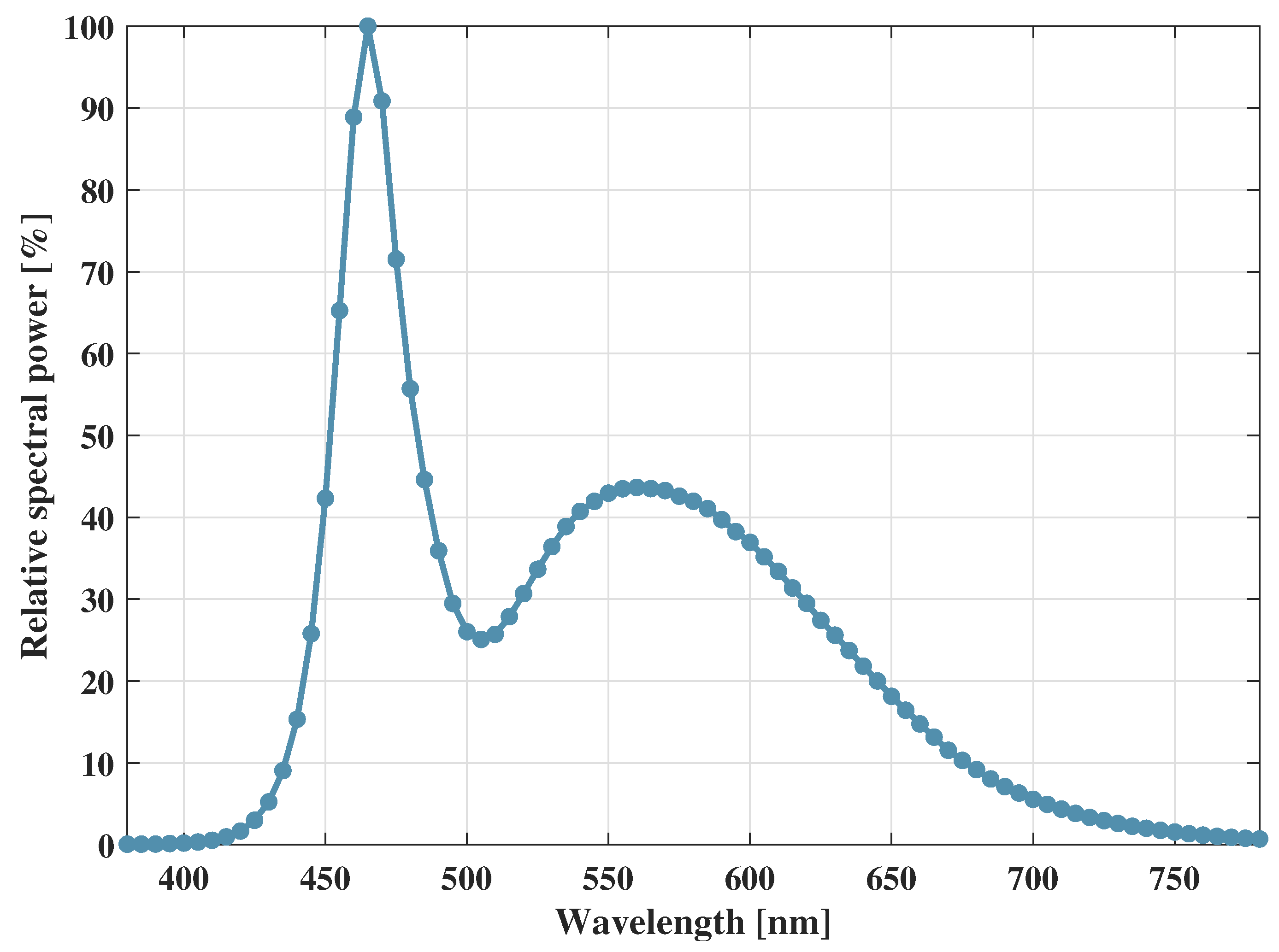
2.3. Ray-Tracing Simulation Setup for VLC Bands

We utilized the non-sequential ray-tracing software Zemax® (Zemax LLC, Kirkland, WA, USA) to obtain the VLC channel data [30]. VLC channel models developed using this non-sequential ray-tracing method were accepted as reference channel models in IEEE 802.15.13 and IEEE 802.11bb [22]. This channel modeling approach has been validated through experimental results in [31].
The first step was to construct a three-dimensional simulation environment to recreate the industrial scenario. Firstly, the floor, ceiling, and walls were constructed according to the scenario size. Then, CAD models that matched the actual length, width, and height of the metal instruments were chosen and imported into the software according to their position in the realistic industrial scenario.
Moreover, the reflection characteristics of each object were set according to those of its actual material. The reflection coefficient refers to the ratio of the intensity of the reflected light to the intensity of the incident light on the reflective material surface. It is influenced by the wavelength of the light signal. Due to the large wavelength coverage of visible light signals, the wavelength dependence of the reflection coefficients for various materials needed to be taken into consideration, which is shown in Figure 2. Commonly used materials for indoor scenarios, such as those of the ceiling, floor, and plaster wall, were obtained from [30]. The remaining materials, such as plate window glass, pinewood, galvanized steel, and Fe, were obtained from [32]. Furthermore, the radiation pattern was set based on the roughness of the object. For non-metallic reflectors, which are relatively rough, the pure Lambertian radiation model was adopted. For metal instruments, specular reflection and Lambertian radiation simultaneously occurred, with each accounting for a proportion of half of the received power.
The second step was to set up the Tx and Rx in the simulation environment. We placed the Tx and Rx on the same LOS path as that in the electronic wave band simulation. On the Tx side, we utilized the method of splicing multiple LEDs to ensure that the light source and the isotropic antenna in the electronic wave band had the same transmission pattern. Nine commercially available light sources (PAR20) that had a viewing angle of 40 were used to achieve 360 coverage, with different lights pointing from 0 to 360 (interval of 40 ) at TX. Furthermore, the relative spectral power distribution of the light source followed that of typical white light distribution, as shown in Figure 3. On the Rx side, we used rectangular detectors that were facing in the direction of the Tx. All the key parameters can be found in Table 2.

3. Data Processing

In this section, we introduce the channel characteristic parameter extraction method based on the electronic wave band channel data from Wireless InSite® and the VLC channel data from Zemax®. Three types of channel characteristics will be presented, including the path loss, RMS DS, and AS.
For the electronic wave band, the CIR can be given by
h ( τ ) = a 1 δ ( τ τ 1 ) + n = 2 N a n e j ϕ n δ ( τ τ n ) ,
where a 1 presents the deterministic (typically LOS) component with the excess delay τ 1 . The parameters a n , τ n , and ϕ n are the amplitude, excess delay, and initial phase of the nth stochastic (typically NLOS) component, respectively. N denotes the number of multiple paths.
For the visible light band, the CIR can be given by
h ( τ ) = n = 1 N a n δ ( τ τ n ) .
In the following equation, the CIR is utilized to obtain the channel characteristics. The path loss is the reduction in the power density of a radio wave as it propagates, which is of high importance for coverage prediction and interference analysis. According to the definition of the path loss, it can be defined by [33]
P L [ d B ] = 10 log 10 ( n = 1 N h ( τ n ) 2 ) ,
The RMS DS describes the time dispersion of the MPCs, which determines the length of the guard interval in the OFDM system. It can be expressed by
τ R M S = n = 1 N ( τ n τ m e a n ) 2 h ( τ n ) 2 n = 1 N h ( τ n ) 2 ,
in which τ m e a n is the average excess delay, which can be derived by
τ m e a n = n = 1 N τ n h ( τ n ) 2 n = 1 N h ( τ n ) 2 .
The AS can characterize the dispersion degree of MPCs in the angle dimension, which can be used to represent the gain brought by MIMO technology [34]. In this paper, we analyze the angle spread of the arrival for the azimuth dimension, which can be expressed by
σ A S = 2 ln ( n = 1 N e j θ n h ( τ n ) 2 n = 1 N h ( τ n ) 2 ) ,
where θ n is the angle of the MPCs in radians.

4. Results and Analysis
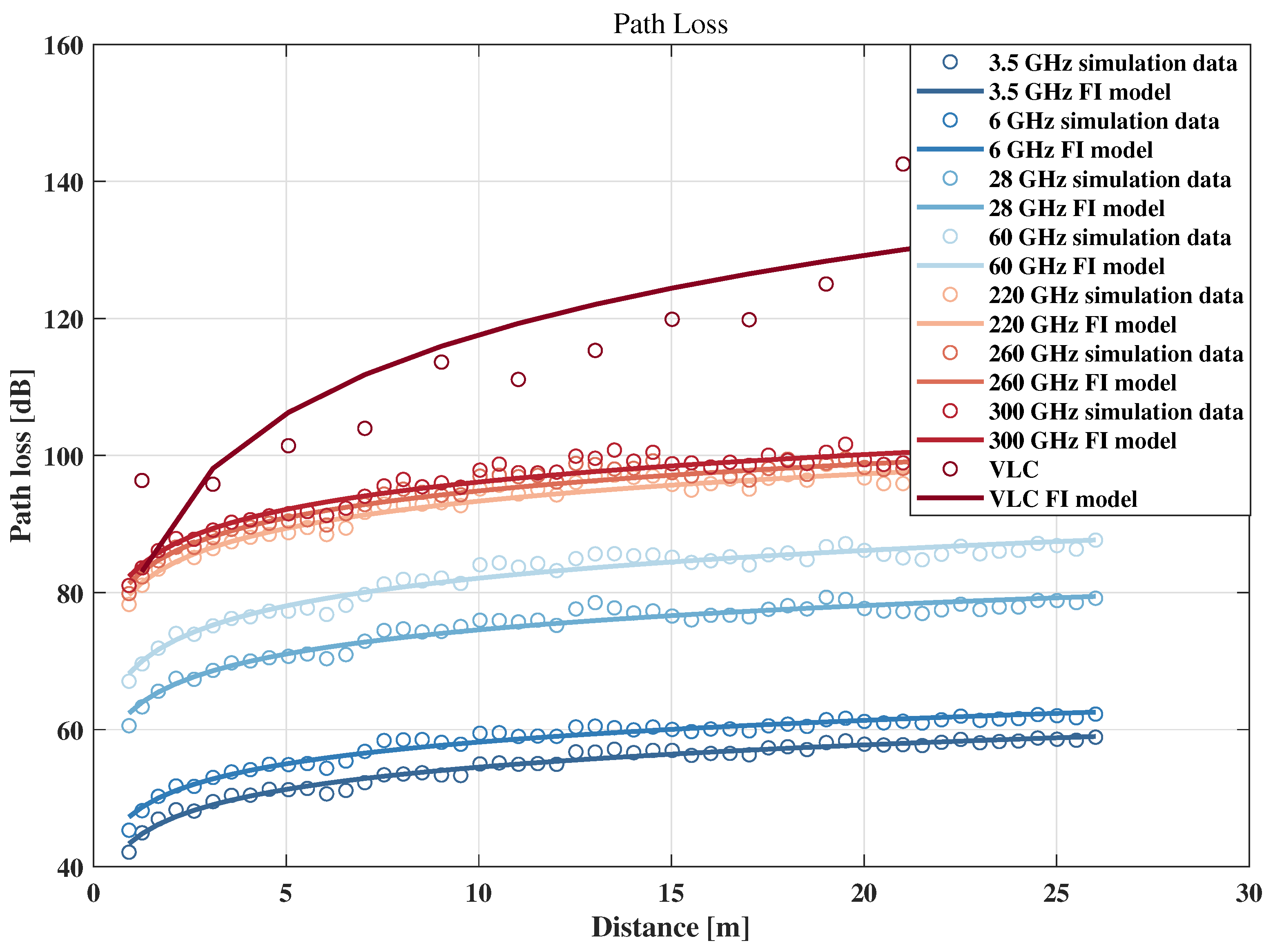
In this section, we analyze the channel characteristics, present the channel characteristic models, and compare the channel characteristic model parameters between the sub-6 GHz, mmWave, THz, and visible light bands. Firstly, the path loss is analyzed and the distance dependency of the path loss is characterized by the FI model. Secondly, the RMS delay spread is analyzed with regard to the distance dependency, and the CDF of the RMS delay spread is modeled. Finally, the azimuth AS is analyzed, and the CDF model of the AS is presented.

4.1. Path Loss

Figure 4 presents the path loss results for all the frequency bands. It was observed that along the LOS path, the path loss for all the frequency bands showed an obvious distance dependence, and the path loss increased with an increasing distance from the transceiver with a non-linear relationship. Moreover, it could be observed that the path loss of the visible light band exhibited more significant variation with the transceiver distance compared with the electronic wave bands, and the path loss variation for various electronic wave bands was similar. For example, when the transceiver distance increased from 3 m to 9 m, the variation in the path loss for the visible light band was 15.5 dB, while the path loss variation for the other electronic wave bands was 6.43, 5.92, 6.49, 6.98, 5.41, 5.12, and 4.55 dB, respectively. This can be attributed to the LOS transmission of VLC. That is, in the received signal, LOS components account for a majority of the received power, while NLOS components only account for a small portion. As the LOS component mainly varies depending on the transceiver distance, the path loss for the visible light channel varies significantly with the transceiver distance.
In addition, at the same transceiver distance, the path loss increased with an increase in the frequency. Specifically, the path loss of the visible light channel was much higher than that of the electronic wave channel in general. At a small transceiver distance, the difference in the path loss between the electronic wave and visible light wave was relatively small. As the transceiver distance increased, the difference in the path loss between the visible light and electronic wave bands grew larger. For example, at a transceiver distance of 2.8 m, the path loss difference between the visible light signal and the 300 GHz signal, which was in the THz band, was only 8.37 dB. When the transceiver distance was 23 m, the path loss difference reached 27.10 dB. This shows that in short-range communication, there is not much difference in performance between THz communication and VLC. For long-range communication, electronic wave communication possesses great advantages over VLC.
In the THz bands, a large frequency change can only bring about small changes in the path loss, and in the mmWave and sub-6 GHz bands, a smaller frequency change will lead to a large path loss difference. For instance, at a transceiver distance of 15 m, the path loss difference between 300 GHz and 220 GHz was only 3.13 dB, while the path loss difference between 60 GHz and 39 GHz was 8.58 dB, and the path loss difference between 6 GHz and 3.5 GHz was 3.07 dB. Therefore, there will be significant differences in the coverage capability when applying different frequency bands, and a strict frequency selection must be made based on the propagation characteristics during deployment.
To accurately characterize the path loss, the FI model was utilized to fit the path loss for all the frequency bands, which can be expressed as
P L F I ( d ) = α + 10 β log 10 d + X σ ,
where α is the floating intercept, β is the slope of the model, which is the PLE, and X σ is a zero-mean Gaussian variable with a standard derivation, σ , representing the shadow effect. The fitting parameters for all the frequency bands are shown in Table 3.
In 3GPP TR 38.901, the channel parameters of the factory scenario are presented, which can support the frequency bands for 0.5–100 GHz. The path loss model parameters in the factory scenario are distinguished based on the density of scatterers and the height of the transmitter. In our research, the simulation scenario had dense metal instruments and high transmitters, which corresponds to the DH scenario with dense clutter and high base stations in 3GPP TR 38.901, and the PLE in 3GPP TR 38.901 is 2.19, which is much higher than that of the electronic wave bands obtained in our research.
This can be attributed to the inconsistent height of the receiver. In 3GPP TR 38.901, the height of the receiver is described as embedded, which represents that the receiver height is the same as the average height of the reflector in the scenario, while in this research, the receiver was located lower than the average height of the metal instruments, which meant that there were a large number of metal reflectors distributed around the receiver. The abundant metal reflectors could lead to various NLOS signals. Therefore, in the received signal, the ratio of the LOS signal was relatively small, resulting in a smaller PLE. This can also be verified by the K factor. In 3GPP TR 38.901, the average K factor for the factory scenario is 7 dB, while in this research, the average K factor for the 3.5 GHz channel was −7.74 dB. The smaller value of the K factor represents a small proportion of LOS power in this research. Therefore, the height of the receiver will also greatly affect the parameters of the path loss model in industrial scenarios, which must be taken into account during path loss modeling.
Furthermore, due to the abundant NLOS signals, the PLE for the industrial scenario is lower than that for the common indoor hotspot scenario for all the electronic wave bands. For instance, for 0.5–100 GHz bands, the PLE for the indoor office scenario is 1.73 in 3GPP TR 38.901. Moreover, for the VLC band, the PLE for the industrial scenario is much higher than that for the common indoor hotspot scenario. For example, in [35], the PLE is 1.70 for the indoor conference scenario, while the PLE for the industrial scenario was 3.84 in this research, which is a similar value to that in [23]. This indicates that the light signals will suffer a faster decay in the industrial scenario. This may be due to the combined effect of the large size of the industrial scenario and the special specular reflection on metal surfaces, which would not happen in an indoor office. On the one hand, the large size makes the reflected light rays take longer paths to the RX. On the other hand, specular reflection reduces the angle of the reflected signal compared to pure Lambertian radiation. Therefore, the difficulty for the reflected signals in reaching the receivers is greatly increased. As the transceiver distance increases, the reflected signals that can reach the receiver decrease significantly, resulting in a significant attenuation of the received power with respect to the transceiver distance.

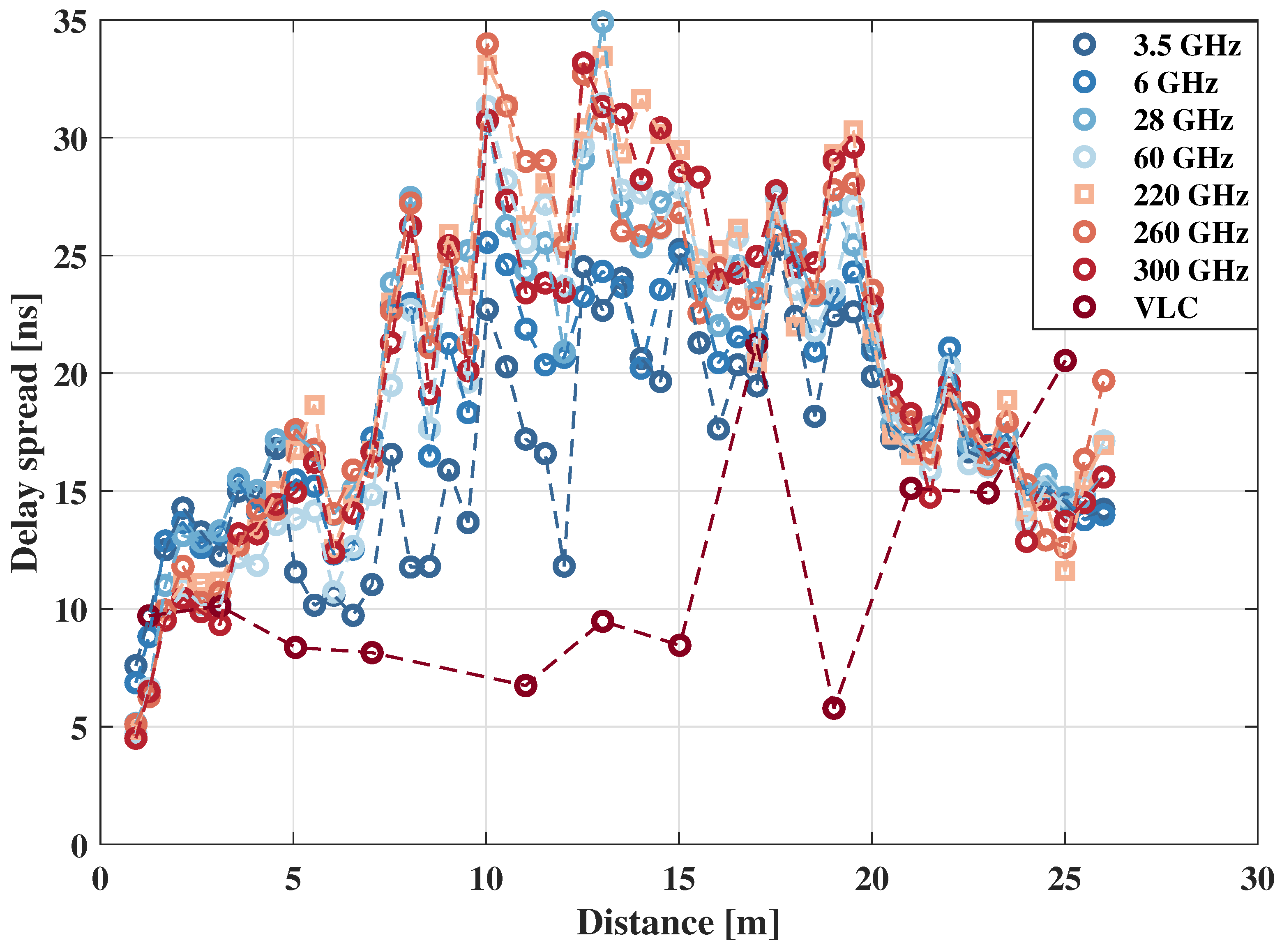
4.2. RMS Delay Spread
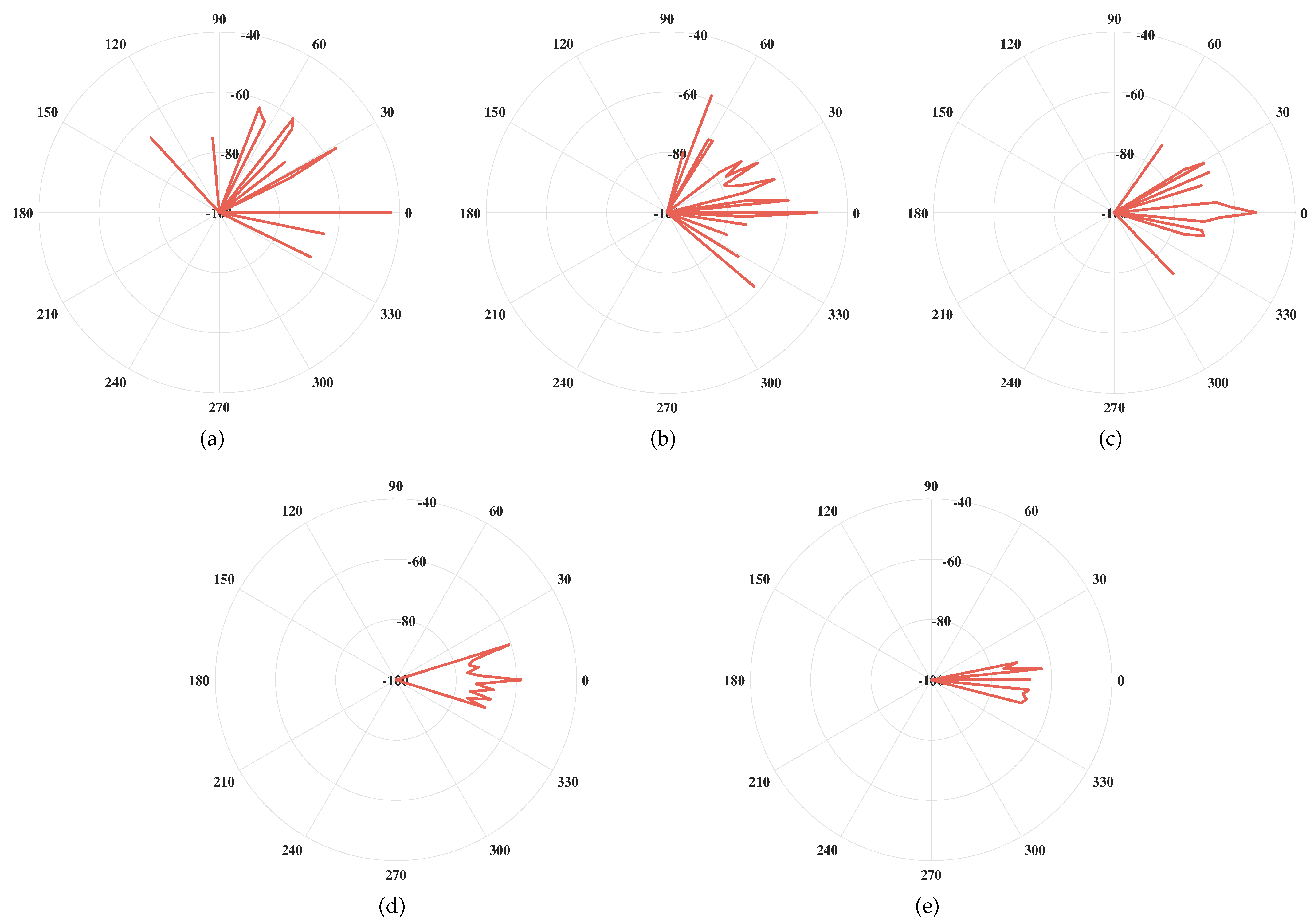
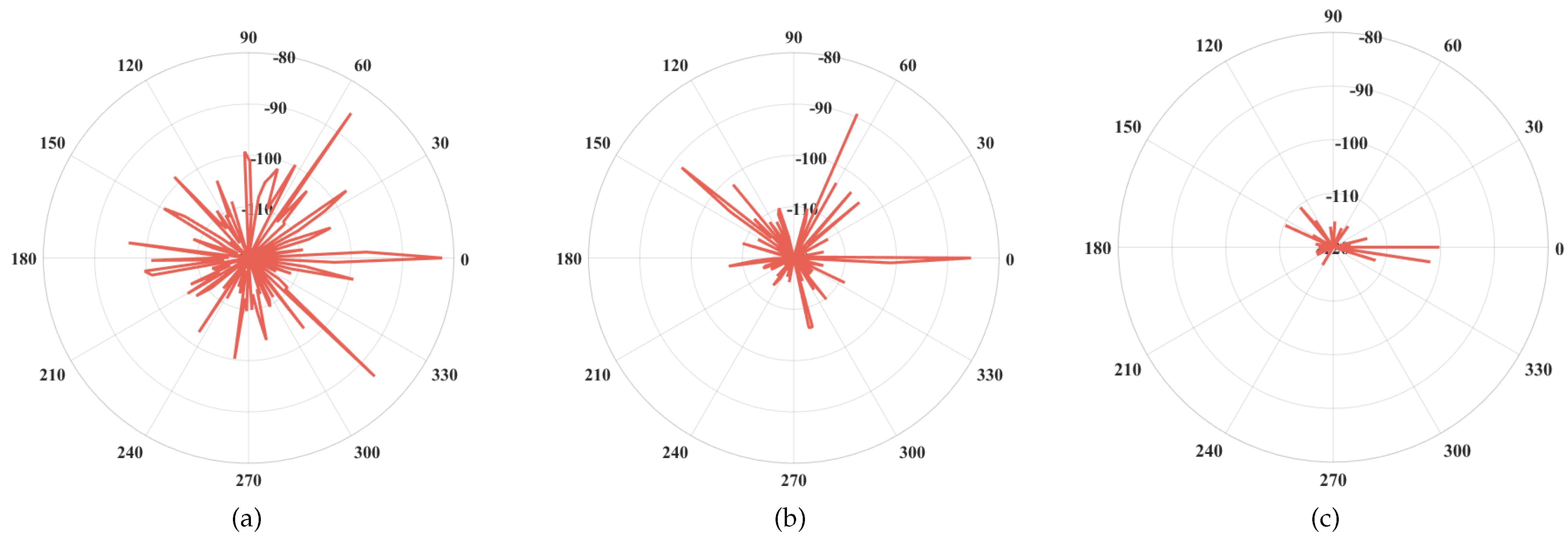
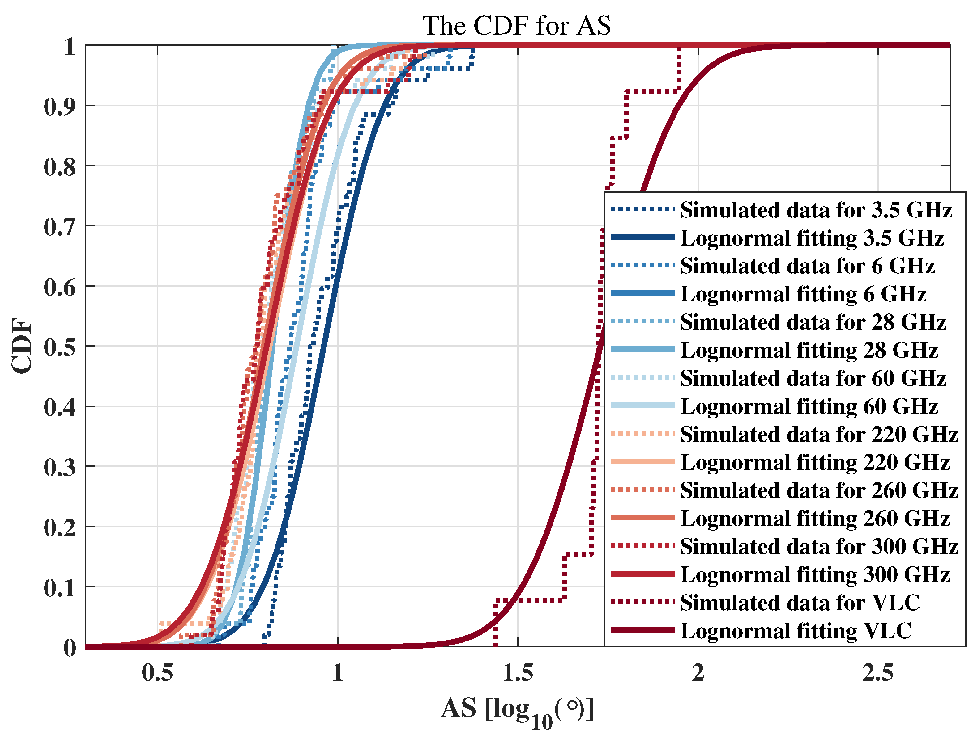
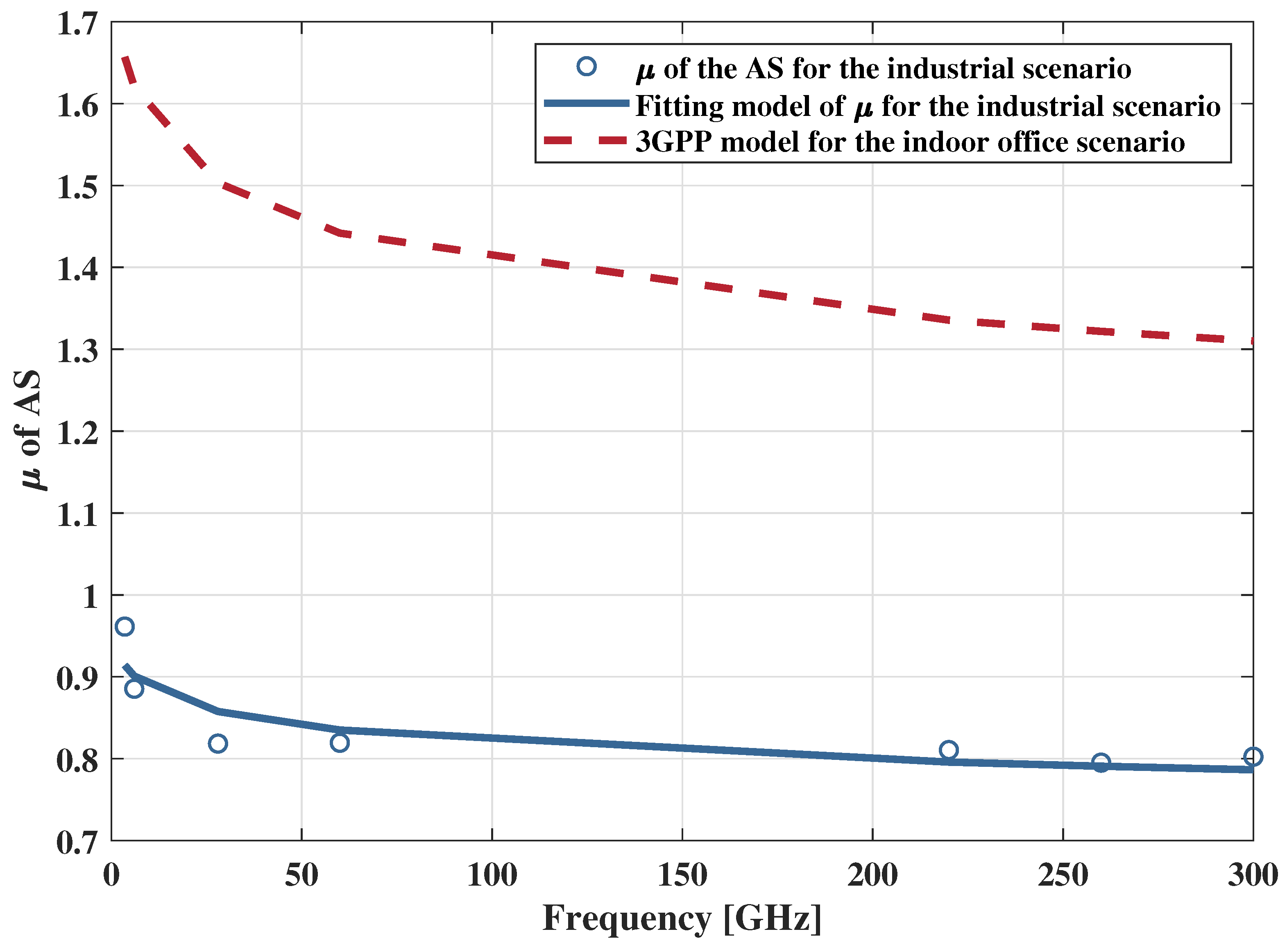
Figure 5 illustrates the RMS DS results in the industrial scenario. Firstly, as the transceiver distance increased, the RMS DS for the electronic wave bands showed an overall trend of first increasing and then decreasing, with the boundary point at a transceiver distance of 13 m. At the receiver closest to the transmitter, only a few NLOS components could be received, and the LOS component power accounted for a large proportion of the received power; thus, the RMS DS was at its minimum. As the transceiver distance increased, the number of NLOS components received from different directions increased, resulting in an increased RMS DS. When the transceiver distance continued to increase and exceeded 13 m, the RMD DS did not increase continuously as in most cases but instead decreased with an increasing distance. This can be attributed to the height of the transceivers, which was lower than the height of most metal instruments on both sides. The high-order reflection MPCs from both sides were obstructed by the metal instruments and could not reach the receivers, and only some low-order reflection rays from the transmitter direction could be received, leading to a decrease in the RMS DS. Therefore, in industrial scenarios, the height of the transmitter and receiver relative to that of the metal equipment can have a great impact on the RMS DS for electronic wave channels. Especially when the scenario size is large, a lower height of the transceiver will lead to a decreasing trend in the RMS DS with an increasing transceiver distance.
For the visible light band, the RMS DS increased with an increase in the transceiver distance. Even when the distance was greater than 13 m, there was no decreasing trend as in the electronic wave bands. This is because visible light signals exhibit Lambertian radiation on the surface of metal objects, and the reflected optical signals will have a wide range of angles. Although the metal instruments on both sides of the receivers may block some of the optical signals from propagating into the surrounding space, multiple reflections will still occur between the two rows of metal instruments. As the distance increases, the received NLOS path increases, resulting in an increase in the RMS DS.
Thirdly, from a frequency perspective, the RMS DS of the visible light band was significantly lower than that of the electronic wave band, while in the electronic wave band, the impact of the frequency on the RMS DS was not significant. On the one hand, the low RMS DS of the visible light band is attributed to the LOS transmission of VLC. The LOS components that have a low time delay account for a large proportion of the received signal power; thus, the RMS DS is relatively small. On the other hand, for the electronic wave band, the distribution of the MPCs that reaches the receiver is similar, which leads to a similar RMS DS. In specular reflection on the surface of metal instruments, the attenuation of signals is relatively small in various frequency bands. There is a low probability that the MPCs experience excessive power attenuation after multiple reflections due to a frequency increase which prevents it from reaching the receivers. Therefore, for various electronic wave bands, there is an obvious frequency dependence of the RMS DS.
Finally, it was found that the RMS DS of both the electronic wave and visible light bands could be fitted well by a lognormal distribution, as shown in Figure 6. The fitting parameters are given in Table 4. For the mean of the RMS DS fitting model, that of the visible light channel was obviously lower than that of the electronic wave channel, which was −7.93 log 10 ( s ) . In the electronic wave bands, the value of μ was not significantly changed with the frequency, ranging from −7.72 to −7.79 log 10 ( s ) , with an average value of −7.74 log 10 ( s ) . In 3GPP TR 38.901, the mean of the RMS DS is also a fixed value, which is expressed as
μ D S 3 G P P = log 10 ( 26 × V S + 14 ) 9.53 ,
where V is the hall volume in m 3 and S is the total surface area of the hall in m 2 (walls + floor + ceiling). By substituting the volume and area values of the researched scenario into Equation (8), the mean was obtained as −7.74 log 10 ( s ) , which is the same as the average value of μ in our research. This indicates that the 3GPP model of the RMS DS for the factory scenario can be extended to apply to THz bands. For the standard deviation, the value for the visible light channel was much larger than that of the electronic wave channel, which was 0.23. For electronic wave channels, the standard deviation increased with the frequency, which can be modeled as
σ D S = 0.034 × log 10 ( 1 + f c ) + 0.10 ,
where f c is the frequency. The root mean square error (RMSE) was 0.009, indicating that the proposed model is in good agreement with the simulated data.
Comparing the RMS DS of the industrial scenario with that of indoor hotspot scenarios, it was found that there was only a small difference in the electronic wave band. For example, at 28 GHz, the mean values of the RMS DS for the industrial scenario and the indoor office scenarios were −7.72 log 10 ( s ) and −7.71 log 10 ( s ) , respectively. Furthermore, for the visible light bands, the RMS DS in the industrial scenario was greater than that in the indoor conference scenario, which was −7.93 log 10 ( s ) and −8.13 log 10 ( s ) , respectively. This is because the obstruction of the metal instruments limited the propagation environment of most electronic wave signals to the space between the metal instruments on both sides, and the impact of the scenario on the signals was not significant. In VLC, the optical signal had a larger angle range due to Lambertian radiation, and the effect of obstruction on the signal was relatively small. The influence of the scenario size on the channel characteristics became increasingly prominent. Thus, the industrial scenario, which had a much larger size than that of the indoor conference scenario, had a greater RMS DS.

4.3. Angle Spread

Figure 7 illustrates the AS for all the frequency bands in the industrial scenario. Firstly, the AS of the visible light band was much larger than that of the electronic wave bands. This was due to the different reflection patterns on the surface of metal reflectors for the visible light and electronic wave bands. There are two kinds of reflection patterns for visible light signals on non-smooth metal surfaces: specular reflection and Lambertian radiation. Meanwhile, electronic wave signals mainly undergo specular reflection. In specular reflection, the direction of the reflected signal is singular, while in Lambertian radiation, the direction of the received signal exists within the range of 0–360°. Therefore, the AS for the visible light channel always maintains a high value.
Moreover, in the electronic wave band, the AS slightly decreased with an increase in the frequency bands, and within each frequency band, the difference in the AS was not significant. For example, at a distance of 21.50 m, for the sub-6 GHz bands, the AS for 3.5 GHz and 6 GHz was 0.81 and 0.76 log 10 ( ) , respectively. For the mmWave bands, the AS for 28 GHz and 60 GHz was 0.73 and 0.72 log 10 ( ) , respectively. For the THz bands, the AS for 220, 260, and 300 GHz was 0.68, 0.68, and 0.69 log 10 ( ) , respectively. This is because as the frequency increases, the reflection ability of the signal decreases, and the power of the NLOS signals decreases, resulting in a decrease in the AS.
Secondly, it can be observed that the AS for the electronic wave band channels experienced four stages as the transceiver distance increased. Firstly, at the receiver closest to the transmitter, the power of the LOS path accounted for a large proportion, and the AS was small, as shown in Figure 8a. As the transceiver distance increased to 2 m, the AS increased significantly with an increase in the transceiver distance. On the one hand, the number of NLOS components increased, which led to an increase in the AS. On the other hand, there was a metal instrument with a large size located at the position with a transceiver distance of 2 m, resulting in a series of strong NLOS signals. The strong NLOS signals caused by this large metal instrument can be clearly seen from the power angular spectrum (PAS), as shown in Figure 8b, which caused an increase in the AS by a large margin. Within the transceiver distance range of 2–5 m, the strong NLOS signals caused by this large metal instrument disappeared, and the AS suddenly decreased. Thirdly, as the transceiver distance increased from 5 m to 10 m, the power of the LOS component decreased greatly, and the NLOS components from the metal instruments on both sides gradually intensified, as shown in Figure 8d, resulting in a slow growth in the AS. Finally, when the transceiver distance was greater than 10 m, the AS decreased as the transceiver distance increased. It can be clearly observed from Figure 8e that the angle range of the received signal gradually converged towards the direction of the transmitter. Due to the lower height of the receivers, the blockage effect of the metal instruments on both sides caused the angle of the received signals to continue to be concentrated toward the transmitter, resulting in a continuous decrease in the AS. Therefore, in the industrial scenario, both ultra-large metal equipment and the height of the receivers can have a significant impact on the AS.
For the visible light channel, the AS almost remained constant with an increasing transceiver distance and was mainly distributed between 1.6 and 1.8 log 10 ( ) . It can be seen from Figure 9 that there were MPCs with high power distributed randomly in the range of 0–360° at each receiver for the visible light band, which kept the AS in a stable state.
Furthermore, we used curve-fitting tools to fit the AS data and found that the AS in both the visible light and electronic wave channels followed a lognormal distribution, as shown in Figure 10. The fitting parameters are shown in Table 5.
For the mean of the AS fitting model, the value for the visible light band was much higher than that for the electronic wave band, which was 1.73 ( log 10 ( ) ) . In the electronic wave band, the mean had a decreasing trend with an increasing frequency, as shown in Figure 11, which can be modeled as
μ A S e l e = 0.07 × log 10 ( 1 + f c ) + 0.96 .
The RMSE was 0.031, indicating that the proposed model has a goodness of fit to the simulated data. For the standard deviation, the value of the visible light band was higher than that of the electronic wave band, which was 0.17. In the electronic wave band, the minimum value of the standard deviation was 0.07 at 28 GHz. At other electronic wave frequencies, the standard deviation values varied between 0.12 and 0.14, with little difference and an average of 0.1234.
Comparing the AS model of the industrial scenario with that of indoor hotspot scenarios in 3GPP TR 38.901, it was found that for the electronic wave band, the μ of the industrial scenario was much lower than that of the indoor office scenario. This was due to the blockage effect of the metal instruments caused by the lower height of the receivers. For the visible light band, there is no proposed model of the AS in the existing study. In [36], the median of the measured AS in the office was 1.40 ( log 10 ( ) ) , which is lower than the μ in the industrial scenario. This is due to the fact that the abundant metal instruments generated rich reflection signals which improved the AS.

5. Conclusions

In this paper, we conducted a comprehensive comparison of the channel characteristics for all the frequency bands, including sub-6 GHz, mmWave, THz, and VLC, in the industrial scenario. Firstly, the channel characteristics, including the path loss, RMS DS, and AS, were analyzed with respect to the frequency dependence and the distance dependence. On the one hand, the visible light band exhibited significant differences in channel characteristics compared to the electronic wave band. Due to the LOS transmission of VLC, the visible light band had a higher path loss, and the path loss exponent reached 3.84. Due to the Lambertian radiation pattern, which has a wide range of reflection angles, the AS of the visible light band was much larger than that of the electronic wave band, which was 1.73 ( log 10 ( ) ) and 0.80 ( log 10 ( ) ) for the visible light and THz bands, respectively. On the other hand, the blockage effect of the metal instruments in the industrial scenario will greatly affect the channel characteristics. As the transceiver distance grows large, signals from both sides of the receiver will be blocked by metal instruments, resulting in a decreasing trend in the RMS DS for the electronic wave band.
Secondly, the statistical characteristics of the channel properties were analyzed and modeled. It was found that both the RMS DS and the AS could be well fitted by the lognormal function for all the frequency bands. For the mean of the RMS DS fitting model, the value for the visible light band was −7.93 ( log 10 ( s ) ) , which was obviously lower than that of the electronic wave bands. In the electronic wave bands, the value of the mean was not significantly changed with the frequency and could be modeled as a constant with the value of −7.74 ( log 10 ( s ) ) . For the mean of the AS fitting model, the value for the visible light band was 1.73 ( log 10 ( ) ) , which was much higher than that for the electronic wave band. In the electronic wave band, the mean of the AS had a decreasing trend with an increasing frequency, which could be modeled as a logarithmic function.
Finally, the proposed statistical parameters of the channel characteristics were compared with the 3GPP TR 38.901 standard. It was found that the height of the receiver caused a larger PLE and a lower AS in the electronic wave bands in our research compared with those in 3GPP TR 38.901. For the RMS DS, the 3GPP model parameter for the factory scenario can be extended to apply to THz bands. What is more, the channel characteristics of the industrial scenario were compared with those of the indoor hotspot scenario. For the electronic wave bands, the channel characteristics of the industrial scenario exhibited a lower PLE, similar RMS DS, and lower AS. For the visible light bands, the channel characteristics of the industrial scenario exhibited a greater PLE, greater RMS DS, and larger AS. This study can provide insights for the evaluation and standardization of multi-frequency communication technology in industrial scenarios.

Author Contributions

P.T., J.Z., and Z.H. are my instructors and gave me full guidance and English correction during the writing process. Then, Y.Y. carried out the related work, including the construction of the simulation environment, the analysis of the simulation data, and the writing of the original draft. T.J., L.X., and G.L., as experts in VLC channel modeling in the company, also provided a lot of guidance on modeling during the data analysis. All authors have read and agreed to the published version of the manuscript.

Funding

This research was supported in part by the National Key Research and Development Program of China (2023YFB2904805), National Natural Science Foundation of China (62201086), Beijing Municipal Natural Fund (L243002), National Natural Science Foundation of China (62341128), Beijing University of Posts and Telecommunications China Mobile Research Institute Joint Innovation Center (CMYJY-202300305), and State Key Laboratory of Information Photonics and Optical Communications (Beijing University of Posts and Telecommunications) (No. IPOC2023ZT02), China.

Institutional Review Board Statement

Not applicable.

Informed Consent Statement

Not applicable.

Data Availability Statement

The data are contained within the article.

Acknowledgments

The authors would like to thank Baobao Liu, Yu Tong, and Shuo Liu for their help in preparing and writing this paper.

Conflicts of Interest

The authors Tao Jiang, Liang Xia, and Guangyi Liu were employed by the China Mobile Research Institute. The remaining authors declare that the research was conducted in the absence of any commercial or financial relationships that could be construed as a potential conflict of interest.

References

  1. ITU-R. Framework and Overall Objectives of the Future Development of IMT for 2030 and Beyond. 2023. Available online: https://www.itu.int/dms_pub/itu-d/oth/07/31/D07310000090015PDFE.pdf (accessed on 20 January 2025).
  2. Tang, P.; Yin, Y.; Tong, Y.; Liu, S.; Li, L.; Jiang, T.; Wang, Q.; Chen, M. Channel Characterization and Modeling for VLC-IoE Applications in 6G: A Survey. IEEE Internet Things J. 2024, 11, 34872–34895. [Google Scholar] [CrossRef]
  3. Tang, P.; Zhang, J.; Xu, H.; Miao, H.; Liu, X. Preliminary perspectives on 3GPP standardization of the propagation channel model for FR3 bands for NR. Sci. China Inf. Sci. 2025, 68, 137301. [Google Scholar] [CrossRef]
  4. Zhang, J.; Zhang, Y.; Yu, Y.; Xu, R.; Zheng, Q.; Zhang, P. 3-D MIMO: How Much Does It Meet Our Expectations Observed from Channel Measurements? IEEE J. Sel. Areas Commun. 2017, 35, 1887–1903. [Google Scholar] [CrossRef]
  5. Miao, H.; Zhang, J.; Tang, P.; Tian, L.; Zhao, X.; Guo, B.; Liu, G. Sub-6 GHz to mmWave for 5G-Advanced and Beyond: Channel Measurements, Characteristics and Impact on System Performance. IEEE J. Sel. Areas Commun. 2023, 41, 1945–1960. [Google Scholar] [CrossRef]
  6. Wang, Y.; Jiang, T.; Tang, P.; Song, Q.; Zhao, X.; Tian, L.; Zhang, J.; Liu, B. Measurement-based analysis and modeling of channel characteristics in an industrial scenario at 28 GHz. In Proceedings of the 2021 IEEE 94th Vehicular Technology Conference (VTC2021-Fall), Virtual Conference, 27 September–28 October 2021; pp. 1–5. [Google Scholar]
  7. Aung, S.M.Y.; Pattanaik, K.K. Path loss measurement for wireless communication in industrial environments. In Proceedings of the 2020 International Conference on Computer Science, Engineering and Applications (ICCSEA), Gunupur, India, 13–14 March 2020; pp. 1–5. [Google Scholar]
  8. Cebecioglu, B.; Mo, Y.K.; Dinh-Van, S.; Fowler, D.S.; Evans, A.; Sivanathan, A.; Kampert, E.; Ahmad, B.; Higgins, M.D. Sub-6 GHz channel modeling and evaluation in indoor industrial environments. IEEE Access 2022, 10, 127742–127753. [Google Scholar] [CrossRef]
  9. Kim, J.; Kim, C.-S.; Hong, J.-Y.; Lim, J.-S.; Chong, Y.-J. Propagation characteristics of an industrial environment channel at 4.1 GHz. In Proceedings of the 2021 International Conference on Information and Communication Technology Convergence (ICTC), Jeju Island, Republic of Korea, 20–22 October 2021; pp. 1530–1532. [Google Scholar]
  10. Solomitckii, D.; Orsino, A.; Andreev, S.; Koucheryavy, Y.; Valkama, M. Characterization of mmWave channel properties at 28 and 60 GHz in factory automation deployments. In Proceedings of the 2018 IEEE Wireless Communications and Networking Conference (WCNC), Barcelona, Spain, 15–18 April 2018; pp. 1–6. [Google Scholar]
  11. Chizhik, D.; Du, J.; Valenzuela, R.A.; Otterbach, J.; Fuchs, R.; Koppenborg, J. Path loss and directional gain measurements at 28 GHz for factory automation. In Proceedings of the 2019 IEEE International Symposium on Antennas and Propagation and USNC-URSI Radio Science Meeting, Atlanta, GA, USA, 7–12 July 2019; pp. 2143–2144. [Google Scholar]
  12. Ito, S.; Hayashi, T.; Yamazaki, K.; Nakao, M.; Sakai, S.; Kurosawa, Y.; Matsunaga, A.; Yoshida, K. Measurement and Modeling of Propagation Characteristics for an Indoor Environment in the 28 GHz-band. In Proceedings of the 2019 IEEE 30th Annual International Symposium on Personal, Indoor and Mobile Radio Communications (PIMRC), Istanbul, Turkey, 8–11 September 2019; pp. 1–6. [Google Scholar]
  13. Qin, Y.; Tang, P.; Tian, L.; Lin, J.; Chang, Z.; Liu, P.; Zhang, J.; Jiang, T. Time-Varying Channel Measurement and Analysis at 105 GHz in an Indoor Factory. In Proceedings of the 2024 18th European Conference on Antennas and Propagation (EuCAP), Glasgow, UK, 17–22 March 2024; pp. 1–5. [Google Scholar]
  14. Ju, S.; Xing, Y.; Kanhere, O.; Rappaport, T.S. Sub-terahertz channel measurements and characterization in a factory building. In Proceedings of the ICC 2022-IEEE International Conference on Communications, Seoul, Republic of Korea, 16–20 May 2022; pp. 2882–2887. [Google Scholar]
  15. Ju, S.; Shakya, D.; Poddar, H.; Xing, Y.; Kanhere, O.; Rappaport, T.S. 142 GHz sub-terahertz radio propagation measurements and channel characterization in factory buildings. IEEE Trans. Wirel. Commun. 2023, 23, 7127–7143. [Google Scholar] [CrossRef]
  16. Ju, S.; Rappaport, T.S. Statistical channel model of Wideband sub-THz radio propagation in indoor factories at 142 GHz: Towards 6G industrial wireless networks. IEEE Trans. Wirel. Commun. 2024, 23, 16316–16331. [Google Scholar] [CrossRef]
  17. Liao, X.; Fan, L.; Wang, Y.; Yu, Z.; Wang, G.; Chen, Y.; Zhang, J. Measurement-Based Channel Characterization in Indoor IIoT Scenarios at 220 GHz. In Proceedings of the 2024 IEEE Wireless Communications and Networking Conference (WCNC), Dubai, United Arab Emirates, 21–24 April 2024; pp. 1–6. [Google Scholar]
  18. Schultze, A.; Schmieder, M.; Wittig, S.; Klessig, H.; Peter, M.; Keusgen, W. Angle-resolved THz channel measurements at 300 GHz in an industrial environment. In Proceedings of the 2022 IEEE 95th Vehicular Technology Conference: VTC2022-Spring, Helsinki, Finland, 19–22 June 2022; pp. 1–7. [Google Scholar]
  19. Elesina, V.V.; Reinhardt, C.E.; Kürner, T. Channel Measurements in Workspace with Robotic Manipulators at 300 GHz and Recent Results. In Proceedings of the 2024 18th European Conference on Antennas and Propagation (EuCAP), Glasgow, UK, 17–22 March 2024; pp. 1–5. [Google Scholar]
  20. Dupleich, D.; Ebert, A.; Völker-Schöneberg, Y.; Löser, L.; Boban, M.; Thomä, R. Spatial/temporal characterization of propagation and blockage from measurements at sub-THz in industrial machines. In Proceedings of the 2023 17th European Conference on Antennas and Propagation (EuCAP), Florence, Italy, 26–31 March 2023; pp. 1–5. [Google Scholar]
  21. Uysal, M.; Miramirkhani, F.; Narmanlioglu, O.; Baykas, T.; Panayirci, E. IEEE 802.15.7r1 Reference Channel Models for Visible Light Communications. IEEE Commun. Mag. 2017, 55, 212–217. [Google Scholar] [CrossRef]
  22. Miramirkhani, F.; Baykas, T.; Elamassie, M.; Uysal, M. IEEE 802.11BB Reference Channel Models For Light Communications. IEEE Commun. Stand. Mag. 2023, 7, 84–89. [Google Scholar] [CrossRef]
  23. Tong, Y.; Tang, P.; Zhang, J.; Liu, S.; Yin, Y.; Liu, B.; Xia, L. Channel Characteristics and Link Adaption for Visible Light Communication in an Industrial Scenario. Sensors 2023, 23, 3442. [Google Scholar] [CrossRef] [PubMed]
  24. Wang, Y.; Lv, Y.; Yin, X.; Duan, J. Measurement-based experimental statistical modeling of propagation channel in industrial IoT scenario. Radio Sci. 2020, 55, 1–14. [Google Scholar] [CrossRef]
  25. Bhatia, G.; Corre, Y.; Di Renzo, M. Tuning of ray-based channel model for 5G indoor industrial scenarios. In Proceedings of the 2023 IEEE International Mediterranean Conference on Communications and Networking (MeditCom), Dubrovnik, Croatia, 4–7 September 2023; pp. 311–316. [Google Scholar]
  26. Dupleich, D.; Ebert, A.; Völker-Schöneberg, Y.; Sitdikov, D.; Boban, M.; Samara, L.; Del Galdo, G.; Thomä, R. Characterization of Propagation in an Industrial Scenario from Sub-6 GHz to 300 GHz. In Proceedings of the 2023 IEEE Globecom Workshops (GC Wkshps), Kuala Lumpur, Malaysia, 4–8 December 2023; pp. 1475–1480. [Google Scholar]
  27. Wang, Y.; Wang, C.; Zheng, X.; Hao, X.; Liao, X. Multi-Frequency Wireless Channel Measurements and Characterization in Indoor Industrial Scenario. IEEE Internet Things J. 2024, 11, 38455–38468. [Google Scholar] [CrossRef]
  28. 3rd Generation Partnership Project (3GPP). Technical Specification Group Radio Access Network; Study on Channel Model for Frequencies from 0.5 to 100 GHz. 3GPP TR 38.901. 2019. Available online: https://www.3gpp.org (accessed on 20 March 2024).
  29. Yuan, Z.; Lyu, Y.; Zhang, J.; Tang, P.; Liu, X.; Lin, J.; Petersen, S.S.; Fan, W. Sub-THz Ray Tracing Simulation and Experimental Validation for Indoor Scenarios. In Proceedings of the 2023 IEEE International Mediterranean Conference on Communications and Networking (MeditCom), Dubrovnik, Croatia, 4–7 September 2023; pp. 7–11. [Google Scholar]
  30. Miramirkhani, F.; Uysal, M. Channel Modeling and Characterization for Visible Light Communications. IEEE Photonics J. 2015, 7, 1–16. [Google Scholar] [CrossRef]
  31. Eldeeb, H.B.; Uysal, M.; Mana, S.M.; Hellwig, P.; Hilt, J.; Jungnickel, V. Channel modelling for light communications: Validation of ray tracing by measurements. In Proceedings of the 2020 12th International Symposium on Communication Systems, Networks and Digital Signal Processing (CSNDSP), Porto, Portugal, 20–22 July 2020; pp. 1–6. [Google Scholar]
  32. ASTER Spectral Library—Version 2.0. Available online: http://speclib.jpl.nasa.gov (accessed on 7 September 2023).
  33. Yin, Y.; Tang, P.; Zhang, J.; Hu, Z.; Xia, L.; Liu, G. Multi-Wavelength Path Loss Model for Indoor VLC with Mobile Human Blockage. Electronics 2023, 12, 5036. [Google Scholar] [CrossRef]
  34. Tang, P.; Zhang, J.; Miao, H.; Wei, Q.; Zuo, W.; Tian, L.; Jiang, T.; Liu, G. XL-MIMO channel measurement, characterization, and modeling for 6G: A survey. Front. Inf. Technol. Electron. Eng. 2024, 25, 1627–1650. [Google Scholar] [CrossRef]
  35. Liu, B.; Tang, P.; Zhang, J.; Yin, Y.; Liu, G.; Xia, L. Propagation Characteristics Comparisons between mmWave and Visible Light Bands in the Conference Scenario. Photonics 2024, 9, 228. [Google Scholar] [CrossRef]
  36. Liu, S.; Tang, P.; Zhang, J.; Yin, Y.; Tong, Y.; Liu, B.; Liu, G.; Xia, L. Statistical channel modeling for indoor VLC communications based on channel measurements. China Commun. 2024, 21, 131–147. [Google Scholar] [CrossRef]
Figure 1. Layout of the industrial scenario.
Photonics 12 00257 g001
Figure 2. The reflection coefficients for various materials.
Photonics 12 00257 g002
Figure 3. The relative spectral power distribution of the light source.
Photonics 12 00257 g003
Figure 4. Path loss vs. transceiver distance.
Photonics 12 00257 g004
Figure 5. RMS DS vs. transceiver distance.
Photonics 12 00257 g005
Figure 6. CDF of the RMS DS.
Photonics 12 00257 g006
Figure 7. AS v.s. transceiver distance.
Photonics 12 00257 g007
Figure 8. PAS of the electronic wave channel: (a) d = 1 m, (b) d = 2 m, (c) d = 5 m, (d) d = 10 m, (e) d = 27 m.
Photonics 12 00257 g008
Figure 9. PAS of the VLC channel: (a) d = 5 m, (b) d = 10 m, (c) d = 21 m.
Photonics 12 00257 g009
Figure 10. CDF of the AS.
Photonics 12 00257 g010
Figure 11. The mean value of the lognormal fitting for the AS.
Photonics 12 00257 g011
Table 1. Research progress in channel characteristics at multiple bands in industrial scenarios.
Frequency BandFrequency PointModeling ApproachChannel CharacteristicsInfluence FactorsRef.
Sub-6 GHz2.4 GHzChannel measurementPath lossTransceiver distance[7]
4.145 GHzChannel measurementPath loss, RMS DSEnvironmental density[8]
4.1 GHzChannel measurementPath loss, RMS DSTransceiver distance,
LOS and NLOS cases
[9]
mmWave28 GHzChannel measurementPath loss, RMS DS, ASAntenna height[6]
28 GHzRay-tracing-based simulationPath loss, LOS probabilityEnvironmental density[10]
28 GHzChannel measurementPath lossTransceiver distance,
LOS and NLOS cases
[11]
28 GHzChannel measurementPath loss, RMS DS, ASLOS and NLOS cases[12]
105 GHzChannel measurementPDP, RMS DS, temporal PDP
correlation coefficient
Time-varying channel[13]
142 GHzChannel measurementPath loss, RMS DS, ASPolarization characteristics[14]
142 GHzChannel measurementPath loss, RMS DS, ASAntenna transmission pattern,
antenna height
[15]
142 GHzChannel measurementA 3-D omnidirectional multipath
channel model based on clusters
LOS and NLOS cases[16]
THz220 GHzChannel measurementPath loss, RMS DS, AS,
power delay angle profile
Environmental density[17]
300 GHzChannel measurementPath gain, path loss,
RMS DS, AS
Scenario size[18]
304.2 GHzChannel measurementPath gain, PDP, RMS DSTime-invariant and time-variant
settings, antenna height
[19]
300.7 GHzChannel measurementReceived power, PDPPenetration through glass,
blockage by frame losses
[20]
VLCRay-tracing-based simulationThe channel frequency responses,
channel direct current gain, RMS DS
Comparison of visible light
and infrared frequency bands
[21]
Ray-tracing-based simulationThe channel frequency responses,
channel direct current gain, RMS DS
Various receiving positions[22]
Ray-tracing-based simulationPath loss, RMS DS, ASAntenna height[23]
Multiple bands3–4 GHz and
38–40 GHz
Channel measurementChannel gain coefficient, RMS DS,
and Ricean K factor
LOS and NLOS cases[24]
3.7 GHz and 28 GHzThe Volcano ray-tracing channel
simulation and channel measurement
Channel gain, RMS DS, ASLOS and NLOS cases[25]
6.75 GHz, 74.25 GHz,
and 305.27 GHz
Channel measurementPath loss, normalized power, DSLOS and NLOS cases[26]
28 GHz, 38 GHz,
132 GHz, and 220 GHz
Channel measurementPath loss, RMS DS, AS, K factorScenario size[27]
Table 2. Parameters of simulation setup.
Electronic Wave BandVisible Light Band
Scenario size33.3 m × 7.7 m × 3 m
Average height of metal instruments1.27 m
Central frequency3.5/6/28/60/220/260/300 GHzWhite light (380–780 THz)
TX height1.60 m
TX patternIsotropicIsotropic-like
Analysis rays 10 7
Minimum relative ray intensity 10 3
Transmitter power1 W
Radiation patternSpecular reflectionSpecular reflection 50%
Lambert radiation 50%
RX height1.27 m
RX patternIsotropicRectangular (10 cm)
Table 3. FI model fitting parameters.
Frequency/GHz α β σ
Sub-6 GHz3.543.731.0780.603237
647.631.0540.696649
mmWave2862.821.1740.980498
6068.661.3431.04594
THz22080.131.3211.11161
26081.791.3041.22165
30082.831.331.19503
VLC79.253.8410.1258
3GPP0.5–100 GHz-2.154.00
Table 4. Fitting parameters of lognormal distribution for RMS DS (log10(s)).
Frequency/GHz μ σ
Sub-6 GHz3.5−7.790.12
6−7.750.12
mmWave28−7.720.16
60−7.750.18
THz220−7.720.18
260−7.720.17
300−7.730.19
VLC−7.930.23
Table 5. Fitting parameters of the lognormal distribution for the AS.
Frequency/GHz μ σ
Sub-6 GHz3.50.960.13
60.890.12
mmWave280.820.08
600.820.12
THz2200.810.14
2600.790.13
3000.800.14
VLC1.730.17
Disclaimer/Publisher’s Note: The statements, opinions and data contained in all publications are solely those of the individual author(s) and contributor(s) and not of MDPI and/or the editor(s). MDPI and/or the editor(s) disclaim responsibility for any injury to people or property resulting from any ideas, methods, instructions or products referred to in the content.

