Abstract
When an unmanned aerial vehicle (UAV) tilts to capture an image of a ground target, variations in object distance may lead to uneven resolution distribution, with the focal length ranging from zero to the full field of view. The field-of-view focal length (FFL), which is a function of the field of view, characterizes the optical properties of the system for each viewing angle. The field-of-view focal length (FFL) quantifies the incremental change in image height resulting from marginal rays exiting the optical system, with infinitesimal angular variations at the field boundary. The optical aberration manifests as an effective focal length variation that exhibits field-dependent characteristics. Through systematic calculation and optimization of the field-of-view focal lengths (FFLs) for ground resolution (GR) control, a mid-wave infrared (MWIR) optical system has been successfully designed, featuring a 10° × 8° field of view (FOV) with an F-number of 3. The optical system implements field-adapted focal length adjustment across distinct viewing angles to ensure consistent ground resolution preservation throughout the full field of view. The designed optical system achieves near-diffraction-limited modulation transfer function (MTF) performance across the full field of view, with all dispersion spots consistently confined within the Airy disk at every viewing angle. The optical system demonstrates superior imaging performance with all dispersion spots confined within the Airy disk radius, fully complying with stringent image quality specifications. Featuring a compact structural configuration, the system exhibits optimal suitability for airborne ground-target reconnaissance applications.
1. Introduction
In conventional UAV-based image acquisition, the imaging angle has traditionally been captured in a vertical orientation (orthogonal to the target surface). However, under specific operational conditions—particularly during high-altitude surveillance of obstructed terrain—the UAV-mounted camera fails to maintain a nadir-view alignment, resulting in occlusions of the subjacent target area. Oblique photogrammetry technology effectively addresses the inherent constraints of forward-looking imaging systems in scenarios involving off-nadir ground target acquisition by UAV platforms. Under these imaging conditions, the ground sample distance (GSD) increases toward the edge of the field of view due to the perspective-induced magnification gradient along the optical axis. As a critical intrinsic parameter of optical systems, the focal length exhibits an inverse relationship with the field of view (FOV). Through focal length modulation, a consistent ground sampling distance (GSD) can be maintained across varying viewing geometries, thereby preserving image metric quality. This investigation presents a novel approach for ground sampling distance (GSD) stabilization through the exploitation of spatially variant optical characteristics and the incorporation of freeform optical surfaces, which provide enhanced degrees of freedom for wavefront aberration control. Optical freeform surfaces are defined as non-rotationally symmetric optical surfaces that cannot be described by conventional spherical or aspherical profiles, requiring higher-order parametric representations for accurate characterization [1,2,3]. Freeform optical surfaces offer enhanced design degrees of freedom, facilitating the realization of compact imaging systems with superior aberration correction capabilities, while enabling unconventional form factors that transcend the limitations of traditional rotationally symmetric optics. Freeform optical surfaces can be mathematically represented by four primary formulations: (1) hypocycloidal surfaces, (2) modified aspheric surfaces, (3) bivariate XY polynomial surfaces, and (4) orthogonal Zernike polynomial surfaces [4].
Wu et al. (2019) developed a novel freeform optics design methodology that simultaneously achieved a low F-number and an extended rectangular field of view through advanced field-of-view expansion techniques. The developed optical system achieved a 40° (H) × 30° (V) field of view with controlled maximum relative distortion below 5.5% across the entire imaging plane [5]. Zhu et al. (2019) pioneered the field-of-view focal length concept and implemented a point-by-point iterative ray-tracing algorithm to optimize an airborne oblique imaging system operating in the visible band. The optical system maintains consistent ground sampling distance throughout the imaging field [6]. Wu et al. (2021) developed an off-axis three-mirror freeform imaging system featuring a graded resolution profile (central: high, peripheral: low) across a 30° × 30° FOV, incorporating both field-dependent focal length adaptation and human visual acuity principles. The system achieved a maximum instantaneous field-of-view (IFOV) resolution ratio of 0.47 between the central and peripheral regions [7]. Zhang et al. (2021) developed a varifocal optical system employing field-dependent focal length modulation, featuring a center-to-edge focal length gradient while maintaining a constant F-number across the entire aperture. The system exhibited a 2:1 focal length ratio between the central and peripheral regions [8]. Zhao et al. (2023) developed a compact freeform off-axis three-mirror system (F/2) through nodal aberration theory optimization, achieving diffraction-limited performance. The system configuration comprised a 400 mm entrance pupil diameter with a 2.4° square field of view. The system maintained MTF values ≥ 0.6 at 100 lp/mm across the entire field of view [9]. Chen et al. (2024) developed a fisheye lens system featuring a 160° full FOV with an optimized 50% central FOV, achieving f-tanθ projection consistency through localized focal length adaptation [10].
This study proposes an imaging optical system design with constant ground resolution by utilizing the field-of-view focal length (FFL) concept. The FFL characterizes the local imaging properties at specific field positions, exhibiting angular dependence that reflects both the object-image mapping relationship and local optical characteristics (particularly terrestrial resolution). In contrast, the conventional effective focal length (EFL), derived from paraxial optical theory, serves as a global parameter that determines the system’s overall collimated light convergence capability along with its field of view and magnification ratio. Through precise control of FFL distribution characteristics, we demonstrate a full-field-constant ground resolution design, where this parameter serves as the primary performance metric. This local optical property optimization approach effectively overcomes the inherent limitations of traditional EFL-based global parameterization for specialized imaging applications.
2. System Design Principle
2.1. Optical System Structure Form Selection
Optical systems are typically classified into three fundamental configurations: (1) purely refractive, (2) catadioptric, and (3) all-reflective architectures [11]. The all-reflective optical system utilizes precisely configured mirror assemblies to eliminate refractive effects and minimize wavefront errors, providing effective correction for primary aberrations, including spherical aberration, coma, and chromatic dispersion. This optical configuration significantly improves image fidelity and measurement accuracy, thereby enhancing the telescope’s observational performance. All-reflective optical architectures provide enhanced degrees of freedom for optical parameter optimization, enabling precise customization to meet application-specific performance criteria. Strategic optimization of mirror geometry (including aspheric profiles and radius of curvature) combined with substrate material selection enables enhanced optical throughput and extended spectral bandwidth. All-reflective optical systems have become the preferred solution for spaceborne applications due to their inherent achromatic performance, superior thermal stability, and capability to realize extended focal lengths and large apertures without mass penalties [12].
Reflective optical architectures are primarily categorized into two configurations: (1) coaxial and (2) off-axis designs. Off-axis reflective systems provide broadband achromatic performance with high optical throughput, making them ideal for imaging applications. Off-axis optical configurations eliminate central obscuration by breaking rotational symmetry, at the cost of inducing non-rotationally symmetric aberrations that require specialized correction techniques [13,14]. Conventional spherical and aspherical optical surfaces exhibit limited capability in compensating off-axis aberrations without compromising optimal image quality. Freeform optical surfaces, characterized by their non-rotationally symmetric profiles and enhanced degrees of freedom [15,16], demonstrate exceptional capability in compensating off-axis aberrations [17].
2.2. System Design Indicators
The off-axis three-mirror optical system was designed to meet airborne operational requirements with the following specifications: (1) operational altitude of 2 km, (2) detector pixel pitch of 15 μm, and (3) ground sampling distance (GSD) of 0.53 m, with a corresponding swath width of . The optical system was designed for mid-wave infrared (MWIR) operation, covering the spectral range of 3–5 μm. Key optical parameters, including the effective focal length (EFL) and total field of view (TFOV), can be derived from the following fundamental relationships:
By selecting the central wavelength and substituting the relevant parameters into the diffraction limit equation, the minimum entrance pupil diameter was calculated as . To ensure it was sufficient, it was designed with an actual entrance pupil diameter of 20 mm. The key design specifications are summarized in Table 1.

Table 1.
System performance parameters.
2.3. Establishment of Ideal Object–Image Relationship
The small-image-height method determines the effective focal length by analyzing off-axis ray behavior at infinitesimal field angles (θ→0), where image height (h) scales linearly with field angle. Optical design software implements this parameter as the distortion-referenced focal length (f–D), which characterizes the paraxial focal length derived from distortion analysis at infinitesimal field angles. The small-image-height methodology enables precise characterization of field focal length variations by establishing a differential relationship between infinitesimal field angle increments (Δθ→0) and their corresponding image height displacements, , across the field. Parameter represents the distance between two adjacent pixel centers. Then, the FFL of the system at the field is defined as the ratio of to the tangent of .
The focal length of the field of view, , is
The instantaneous field of view (IFOV) represents the angular extent in object space that corresponds to a single detector pixel’s projection at a given field angle. For rotationally symmetric optical systems, the instantaneous field of view (IFOV) is principally determined by the quotient of the detector pixel pitch and the effective focal length. The instantaneous field of view (IFOV) at a specified field angle is determined through the following computational procedure:
Ground resolution is determined by the instantaneous field of view at each observation angle:
where indicates the working height.
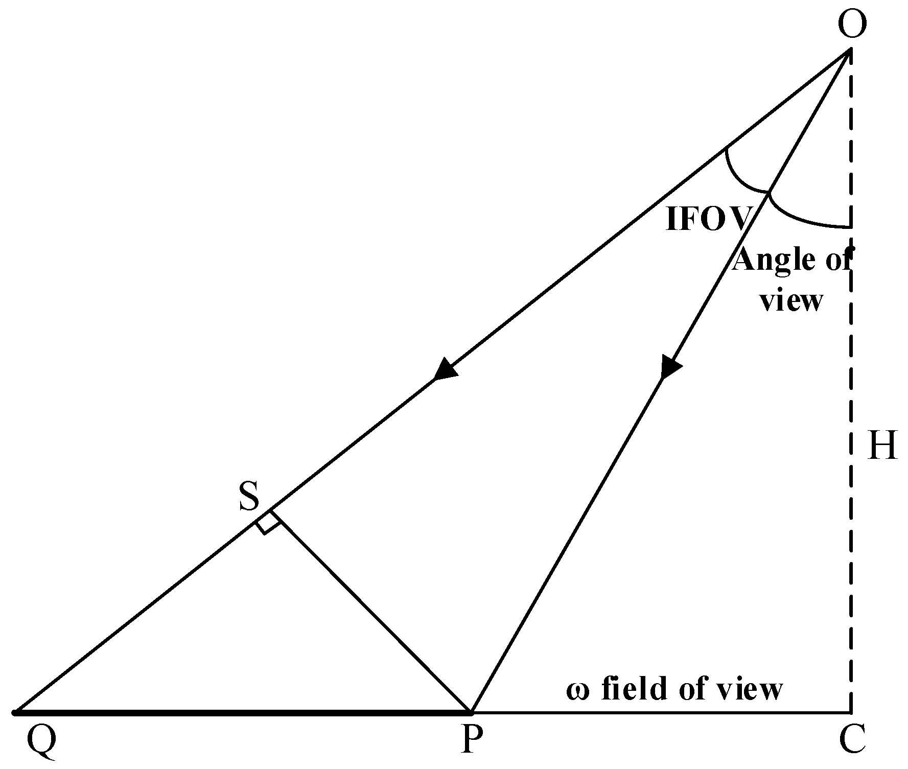
Figure 1 geometrically illustrates the functional relationship between ground resolution and the instantaneous field of view (IFOV) in oblique photography, where represents the platform altitude, denotes the IFOV angle corresponding to (magnified for clarity), the arrows represent the direction of observation, indicates the ground resolution at , and is the associated observation angle. The field of view (FOV) of the system is greater than or equal to 10° or less than or equal to 18°, using a 10° observation angle for distant targets and an 18° FOV for near targets. As the field of view angle increases, the observation point gets closer and closer to the point to be observed. That is, a 10° field of view corresponds to an observation angle of 18°, and an 18° field of view corresponds to an observation angle of 10°, so that the observation angle is . The diagram clearly demonstrates that larger field of view angles result in decreased observation distances.

Figure 1.
Geometric relationship between ground sampling distance and instantaneous field of view.
Correlation between field focal length (FFL) and ground sampling distance (GSD):
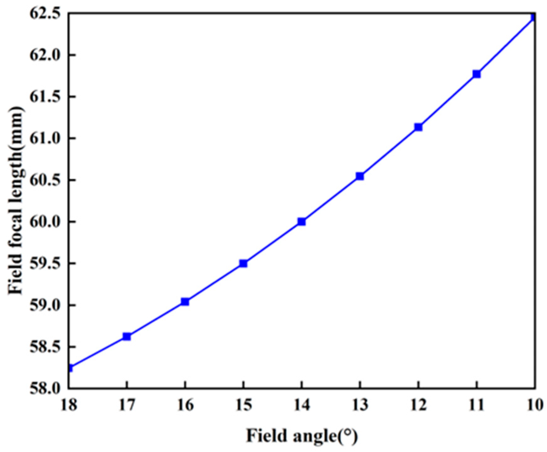
Based on the derived formulation, the required field focal length distribution can be determined by maintaining constant system parameters, to achieve uniform ground resolution (). Consequently, the required field focal length distribution for field angles spanning 10° to 18° can be computationally determined, as presented in Figure 2.

Figure 2.
Computed field focal length (FFL) distribution across specified field angles.
As established by the ideal imaging formulation [18], each field angle in the optical system corresponds to a distinct location of the stigmatic image point. For optical systems operating at infinite conjugate distances, the fundamental imaging relationship can be expressed as:
where denotes the image plane’s tilt angle relative to the X-axis, and represents the Cartesian coordinates of the image plane.
The field focal length distribution, , enables computation of the corresponding image heights, , which establishes a modified object–image correspondence governed by the prescribed focal length variation.
3. Optical System Design
3.1. Calculation of Structural Parameters of Coaxial Three-Mirror Optical System
The off-axis reflection system was derived through off-axis optimization of the coaxial three-mirror system. Therefore, the coaxial three-mirror system must first be calculated based on the design parameters. The configuration of the coaxial three-mirror system is illustrated in Figure 3. Assuming all three reflecting surfaces are quadric, and the object lies at infinity, i.e., , , the coefficient of the distance between the primary mirror and the secondary mirror is defined as , the coefficient of the distance between the secondary mirror and the tertiary mirror is defined as , while and are the magnification of the secondary mirror and the tertiary mirror.

Figure 3.
Initial structure of the coaxial three-mirror system.
Figure 3 illustrates the optical configuration where M1, M2, and M3 represent the primary mirror, secondary mirror, and tertiary mirror, respectively. The parameters h1, h2, and h3 denote the aperture sizes of the primary, secondary, and tertiary mirrors, while d1 indicates the distance between primary and secondary mirrors, and d2 represents the distance between secondary and tertiary mirrors.
The aberration coefficients for spherical aberration, coma, astigmatism, and field curvature of the initial structure were calculated using aberration theory, as follows:
By solving Equations (9)–(16) and setting each aberration coefficient to zero, we adopted a coaxial reflective architecture without an intermediate image plane as our starting configuration. The initial structural parameters were computed by solving the equation system in MATLAB R2021a using the profile parameters, as shown in Table 2. The structural parameters diagram is shown in Figure 4.
Table 2.
Parameters of the coaxial three-mirror inverse structure.

Figure 4.
The 3D structure of the coaxial three-mirror system.
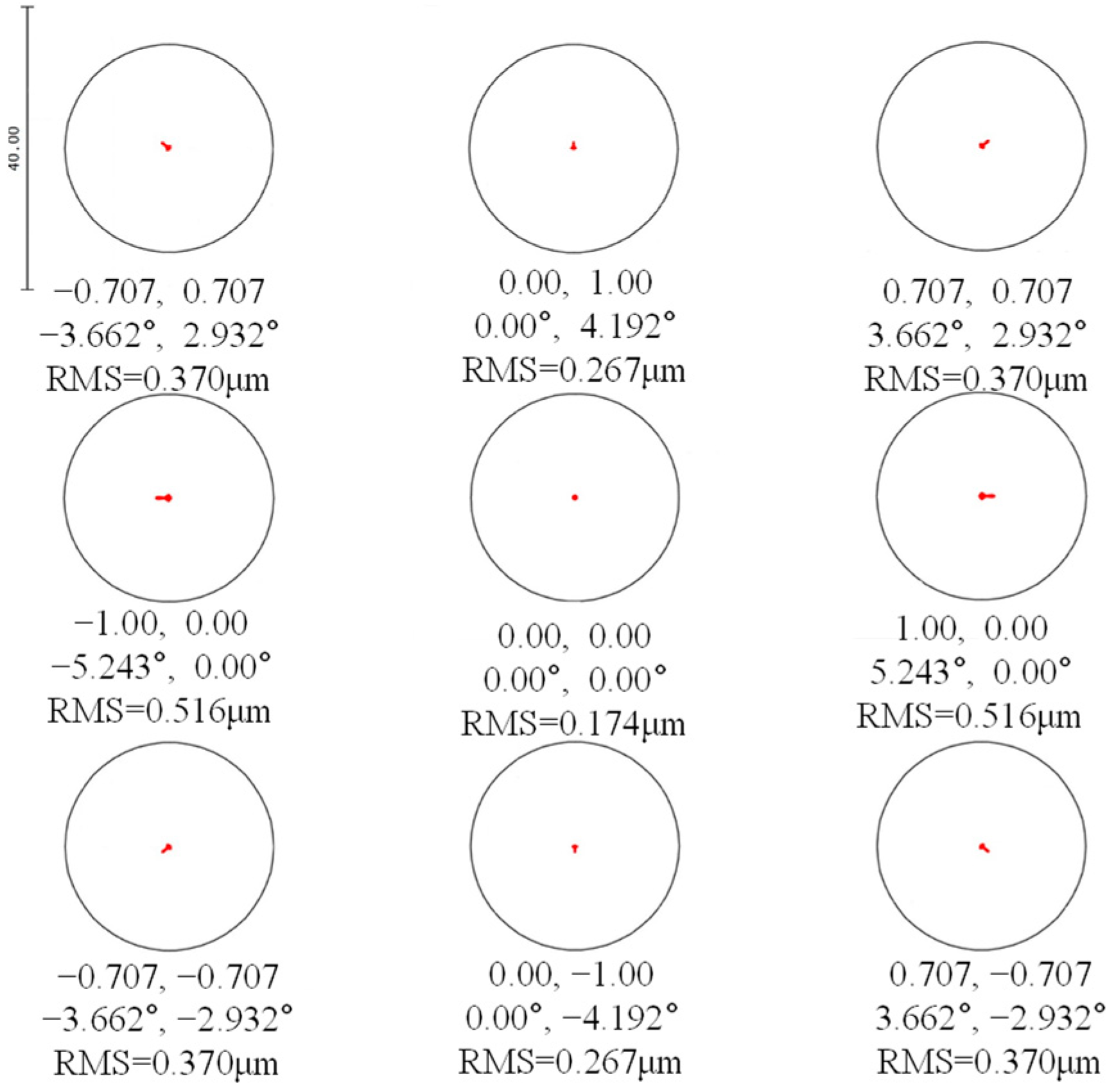
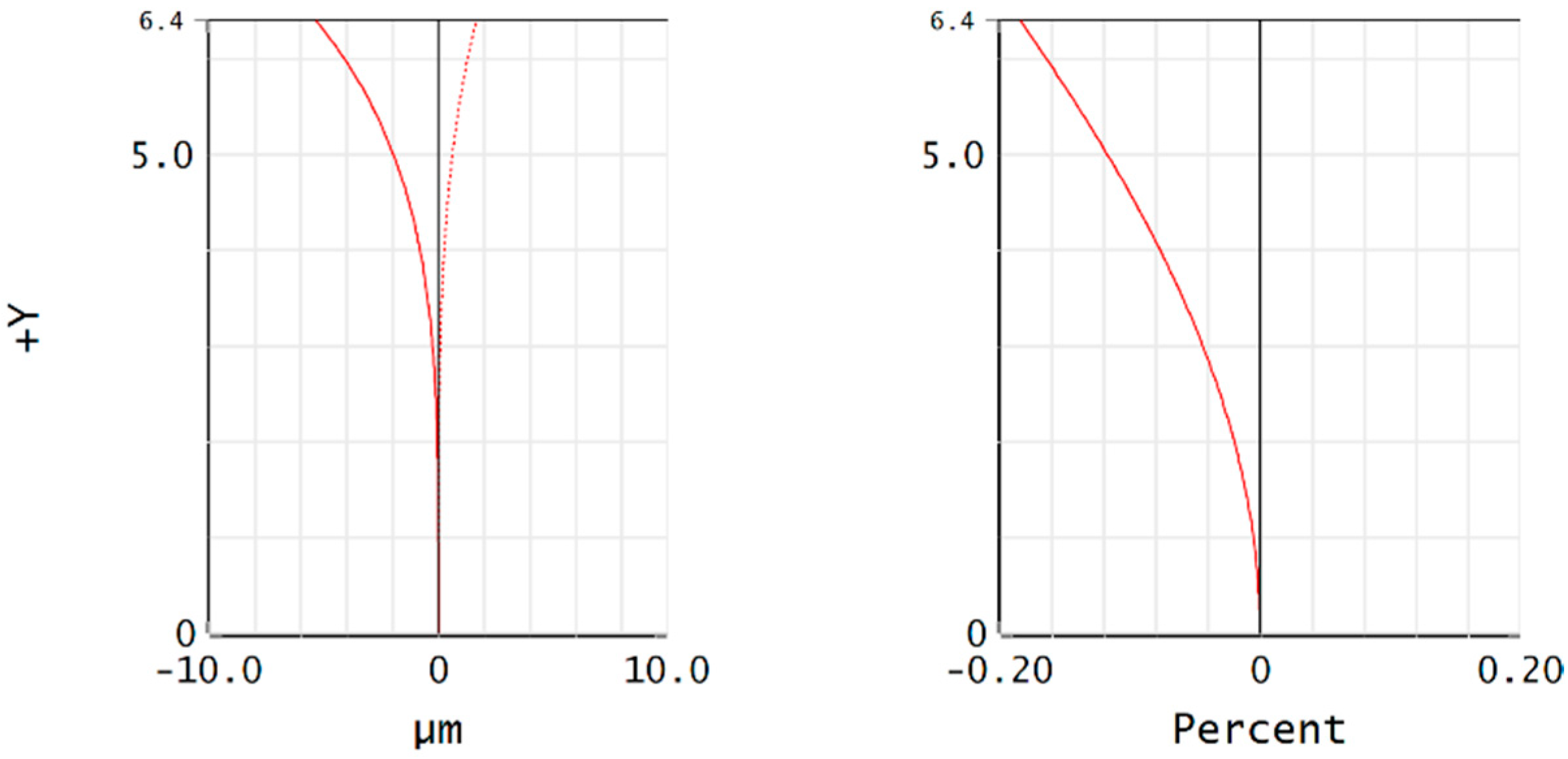
The initial structure’s imaging performance was evaluated. As shown by 0.3 in the system modulation transfer function (MTF) plot in Figure 5, the MTF values for each field of view approached the diffraction limit, indicating great imaging performance. The system’s spot diagram in Figure 6 shows that the diffuse spots were significantly lower than the Airy disk. The system field curvature/distortion diagram in Figure 7 indicates that both the field curvature and distortion were negligible. The initial system exhibited an optimized design suitable for direct implementation in off-axis configurations.

Figure 5.
Plot of the modulation transfer function (MTF) for the coaxial three-mirror system.

Figure 6.
Spot diagram of the coaxial three-mirror system.

Figure 7.
Field curvature and distortion diagram for the coaxial three-mirror system.
In Figure 7, the left plot shows the field curvature of the system, with the vertical axis representing the field of view (FOV) size and the horizontal axis indicating the field curvature value. The red curve depicts the variation of field curvature across the FOV, with a maximum field curvature of 0.8 μm. The right plot presents the distortion characteristics of the system, where the vertical axis denotes the FOV size and the horizontal axis represents the distortion value. The red curve illustrates the distortion variation with respect to the FOV, exhibiting a maximum distortion of 0.0768%.
3.2. Optimized Design
After obtaining the initial structure of the coaxial off-axis process, as required, the off-axis method was categorized into aperture off-axis and field-of-view off-axis. The aperture stop was located on the primary mirror under aperture off-axis conditions, and the optical structure was not symmetrical, so the field of view could not be made too large. In field-of-view off-axis configurations, the aperture stop is typically positioned at the secondary mirror, which is conducive to the expansion of the field-of-view angle. Therefore, this study employed an off-axis field-of-view approach, where the system Y-direction field of view was 10°~18°, and the X-direction field of view was ±5°.
The initial step involved the fundamental system parameters, such as operands like EFFL, WFNO, and others, which were set directly according to the design requirements. The conic coefficient was limited using operands like COVA, ABLT, and others. Aberrations were controlled using operands, such as FCGT, FCGS, TRAY, SPHA, and related mathematical operators.
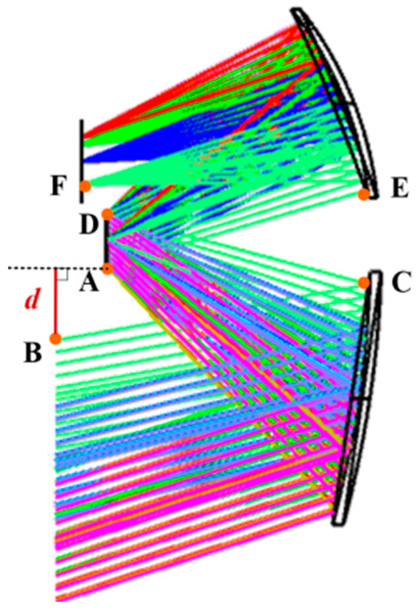
Additionally, the system must avoid becoming coaxial during off-axis optimization, otherwise this could lead to light blockage. To prevent this, the optical system’s structure must be constrained. First, the y-coordinate information of the edge points on the object surface (Surface 1) and the primary mirror (Surface 3) was read to define a straight line. Then, the slope (k) and intercept (b) were calculated using the slope–intercept equation of the straight line, y = kx + b. The y-coordinate information of the edge points beneath the secondary mirror (Surface 5) was then obtained. These coordinates were treated as points, and the distance from each point to the straight line was calculated using Equation (9). A visual representation of this method is shown in Figure 8, where the red line indicates the controlled distance. The off-axis amount was then maintained within the expected range using the PMVA, ABGT, and ABLT operands.

Figure 8.
Schematic diagram of the structural constraints.
Freeform surfaces provide substantial design flexibility for imaging optical systems, making them particularly effective at correcting aberrations in off-axis asymmetric systems. Additionally, they contribute to system miniaturization and weight reduction, decrease the number of components, and enable the realization of parameters, structures, and functions that are challenging to achieve in traditional spherical and aspherical systems. To maintain the system’s constant ground resolution characteristics, this study adopted the XY polynomial expression for the freeform surface.
The fourth-order XY polynomials hold significant practical value in optical design, as they achieve an optimal balance between aberration correction capability and engineering feasibility. These polynomials not only effectively address primary aberrations but also contribute to the suppression of certain higher-order aberrations, fulfilling the imaging demands of most conventional optical systems. Fourth-order terms maintain reasonable computational complexity and align well with modern manufacturing techniques, such as single-point diamond turning (SPDT). When fourth-order correction is insufficient, localized approaches—such as freeform surfaces or region-specific polynomial segmentation—can be employed to enhance performance without resorting to a global increase in polynomial order. This strategy ensures performance goals are met without introducing unnecessary manufacturing or metrological challenges associated with higher-order terms. Thus, a fourth-order XY polynomial was selected to optimize the optical system. Since the optical system is symmetric with respect to the YOZ plane, only the X-even terms in the XY polynomials were adopted.
In order to ensure that the XY polynomial coefficients were consistent with the current processing capacity, the processing was carried out by single-point diamond machining. The one-time first processing accuracy could be controlled at about 0.8 μm, and the RMS value of the first molding could be controlled at about 100 nm. Then, the freeform surface inspection instrument was used for inspection, and compensation processing was carried out after inspection to ensure that the processing accuracy reached λ/50:
In the above equation, the first term represents the aspheric surface type term, denotes the coordinates of the characteristic data points on the unknown surface, c denotes the curvature at the vertex of the fitted surface, k denotes the quadratic surface coefficient (conic coefficient), denotes the term of the free surface of the XY polynomial, and is the coefficient of the corresponding term.
To achieve uniform ground resolution, the y-direction field of view was divided into nine segments for sampling. Light constraints were subsequently applied to the optimized system with high imaging quality. The REAY operand was used to determine the actual image heights for the specified fields of view. The ideal image heights were then calculated using the ideal image-point formula to obtain the perfect image heights for the fields of view. The DIFF operand was used to calculate the deviation between the actual and ideal image heights for each field of view. Finally, the OPGT operand was applied to constrain the difference, with OPLT used to further refine the constraint. To achieve a zero-deviation value, the structure of the freeform off-axis three-mirror optical system will undergo modifications to correct aberrations, ensuring the system meets imaging quality requirements while maintaining a constant ground resolution characteristic. The specific operand settings are shown in Table 3.
Table 3.
Operand settings.
The selection of optimization variables for the system primarily included the curvature radii and conic coefficients of the mirrors, as well as the spacing between each optical element. Thus, these parameters were mainly chosen as optimization variables. The optimization process primarily employed a combination of the default merit function and other operands. There were various default evaluation methods, with spot diagrams and wavefront being the most commonly used. In the initial optimization phase, spot diagrams could be utilized to enhance optimization speed. Once the spot diagrams met certain criteria, wavefront optimization could be adopted in later stages to balance various aberrations.
During optimization, it was essential to effectively control the RMS (root mean square) radius of the spot diagram. The optimization operands for spot diagram size typically included RSCH, RSCE, RSRH, and RSRE. For MTF optimization, operands such as MTFA, MTFT, and MTFS were employed. Additionally, the Seidel coefficients should be examined. If significant spherical aberration or coma is present, operands like SPHA and COMA must be applied for correction.
3.3. Design Results
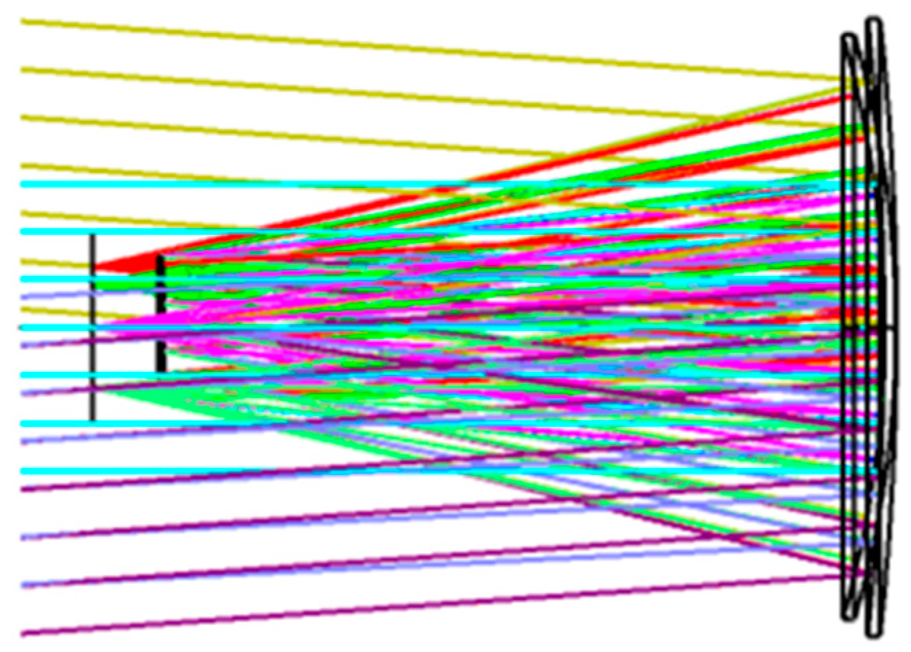
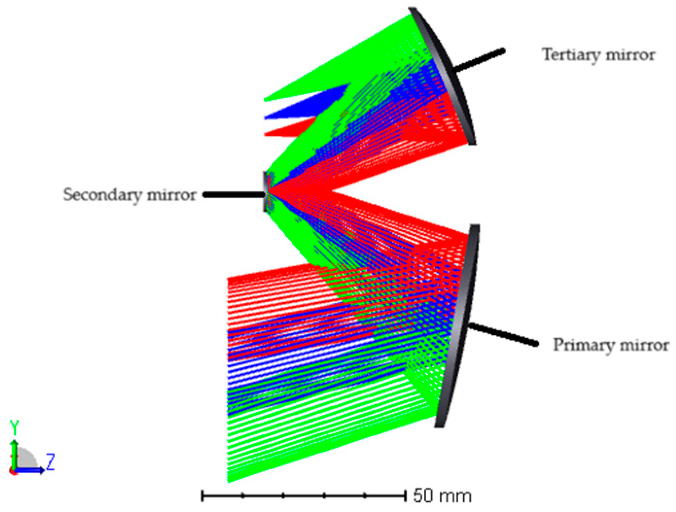
After optimization, the optimized system structure parameters were as presented in Table 4, and the system layout was as illustrated in Figure 9. The design prioritized functional simplicity, as the main mirror and three mirrors could be integrated and manufactured from a single piece of reflective material. This enabled monolithic fabrication of the three primary mirrors, reducing optical system assembly complexity.
Table 4.
Structural parameters of the off-axis three-mirror system.

Figure 9.
Structure of the off-axis three-mirror optical system.
The tertiary mirror employed XY polynomial freeform surfaces to correct off-axis aberrations, thereby ensuring that the final imaging quality requirements were met. The optimized coefficients of the freeform surfaces, expressed as XY polynomials, after optimization, are presented in Table 5.
Table 5.
Three-mirror XY polynomial surface coefficients.
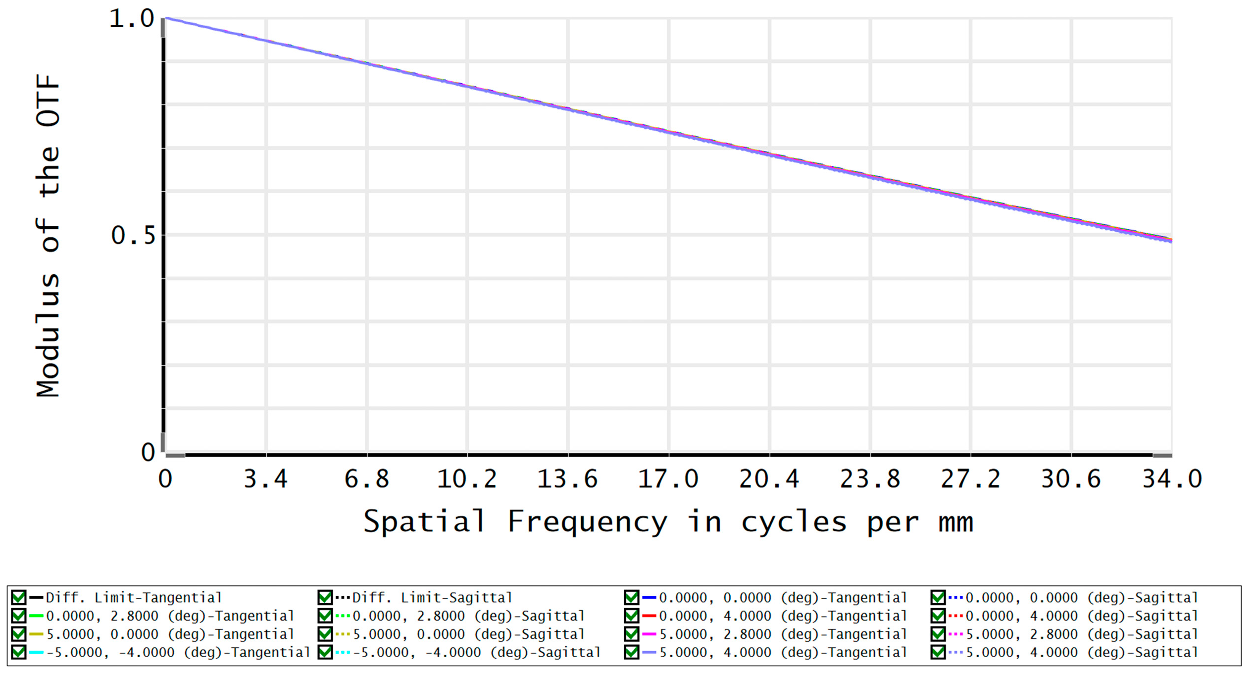
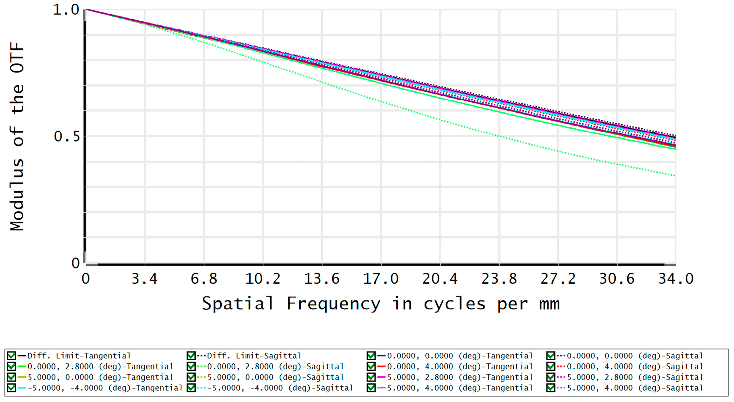
The system used the modulation transfer function (MTF) and spot diagram to evaluate the imaging quality, as shown in Figure 10 and Figure 11. The system exhibited diffraction-limited imaging quality. The MTF curve showed that the optical system can transfer various object frequencies. At a cutoff frequency of 34 lp/mm, the system’s MTF across the full field of view was close to the diffraction limit, with values exceeding 0.4, thus meeting the design specifications.

Figure 10.
MTF of the off-axis three-mirror system.

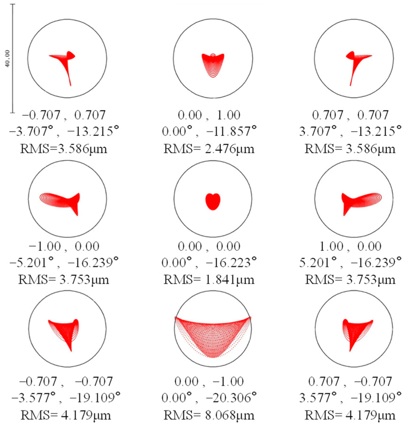
Figure 11.
Spot diagram of the off-axis three-mirror system.
The spot diagram illustrates the optical system’s light convergence ability. The RMS radius serves as a quantitative metric for assessing the system’s imaging performance. As shown in the figure, the maximum RMS radius was 4.985 μm, which meets the imaging requirements, exhibiting a smaller size compared to the detector’s minimum pixel size.
3.4. Tolerance Analysis
Off-axis optical systems do not have symmetry and are susceptible to asymmetric aberrations due to the influence of asymmetric optical elements, which further increases the difficulty of manufacturing and processing the system. Therefore, in order to verify the feasibility of the optical system designed in this paper, a tolerance analysis of the system was required. The average diffraction MTF of the system at 34 lp/mm was used as the evaluation standard to assess the influence of various types of errors of optical elements on the image quality of the system during processing, and the tolerance analysis of the whole system was carried out. The data settings for the tolerance analysis of the system in this paper are shown in Table 6.
Table 6.
Optical system tolerance distribution table.
In the tolerance analysis stage, finite-times Monte Carlo simulation analyses were first carried out using preset tolerance values to identify the key parameters that had the most significant impact on the system performance. Subsequently, these key parameters were optimally tuned to progressively optimize the system performance by shrinking the worst tolerance terms and relaxing the optimal ones. This process was repeated until the system performance was close to the predefined target. After the initial optimization, 200 Monte Carlo simulations were further conducted to fully evaluate the effect of the optimized tolerance settings, and the modulation transfer function (MTF) was used as the main performance evaluation index in this process. The final results of the tolerance analysis are shown in Table 7.
Table 7.
MTF values for system tolerance analysis.
Using Monte Carlo analysis, the results showed that more than 90% of the Monte Carlo samples of this system, after the introduction of errors, had MTF values greater than 0.3, which meets the requirements of industrial production.
In terms of cost, this design used a single-point diamond turning one-shot technique, and the cost of this technique is controllable. The RMS value can be controlled to λ/50, and the roughness can be controlled to within 10 nm.
Mid-wave infrared (MWIR) systems (3–5 μm) exhibited high sensitivity to thermal variations, which can induce undesirable effects, such as thermal expansion and defocusing. To mitigate these issues without resorting to active compensation, passive thermal management strategies can be implemented through careful material selection and mechanical design optimization. Key approaches include (1) employing materials with matched coefficients of thermal expansion (CTE) to minimize thermally induced stresses, (2) incorporating optical compensation structures to maintain focus stability under temperature fluctuations, and (3) integrating flexible mechanical elements to accommodate thermal deformation. Furthermore, the use of high-thermal-conductivity materials enhanced thermal equilibration, thereby reducing temperature gradients and their adverse effects. Notably, refractive optical systems are especially susceptible to thermal perturbations, necessitating stringent application of the aforementioned design considerations to ensure consistent performance.
4. Ground Resolution Analysis
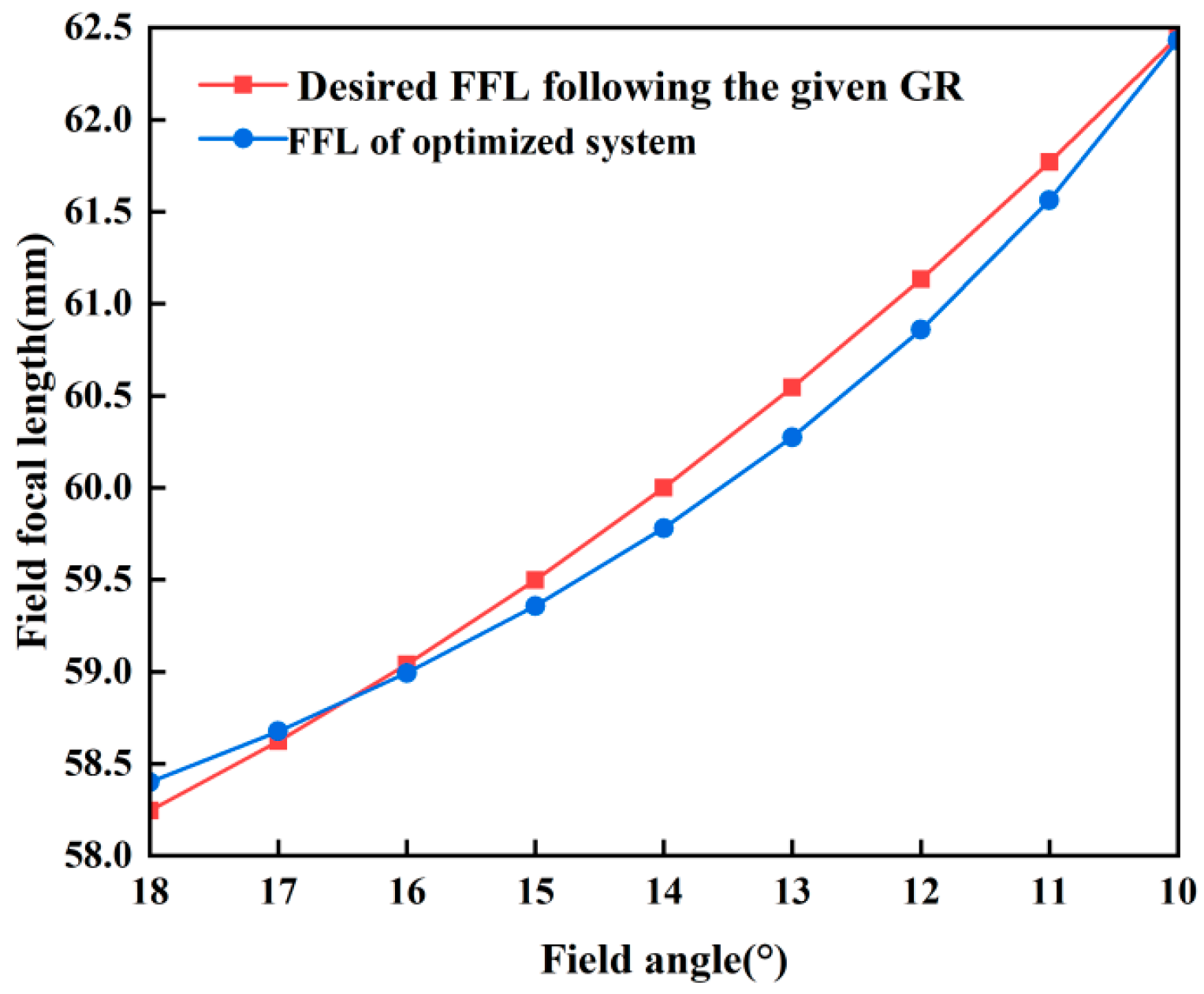
As illustrated in Figure 12, the red curve corresponds to the theoretically derived FFL profile calculated using Equation (10), while the blue curve depicts the optimized FFL distribution obtained through systematic design refinement. The optimized (blue) and theoretical (red) curves demonstrated closely matched ideal profiles, resulting in con-sistent ground resolution (GR) distribution across the field of view.

Figure 12.
Comparison of two different field-of-view focal lengths.
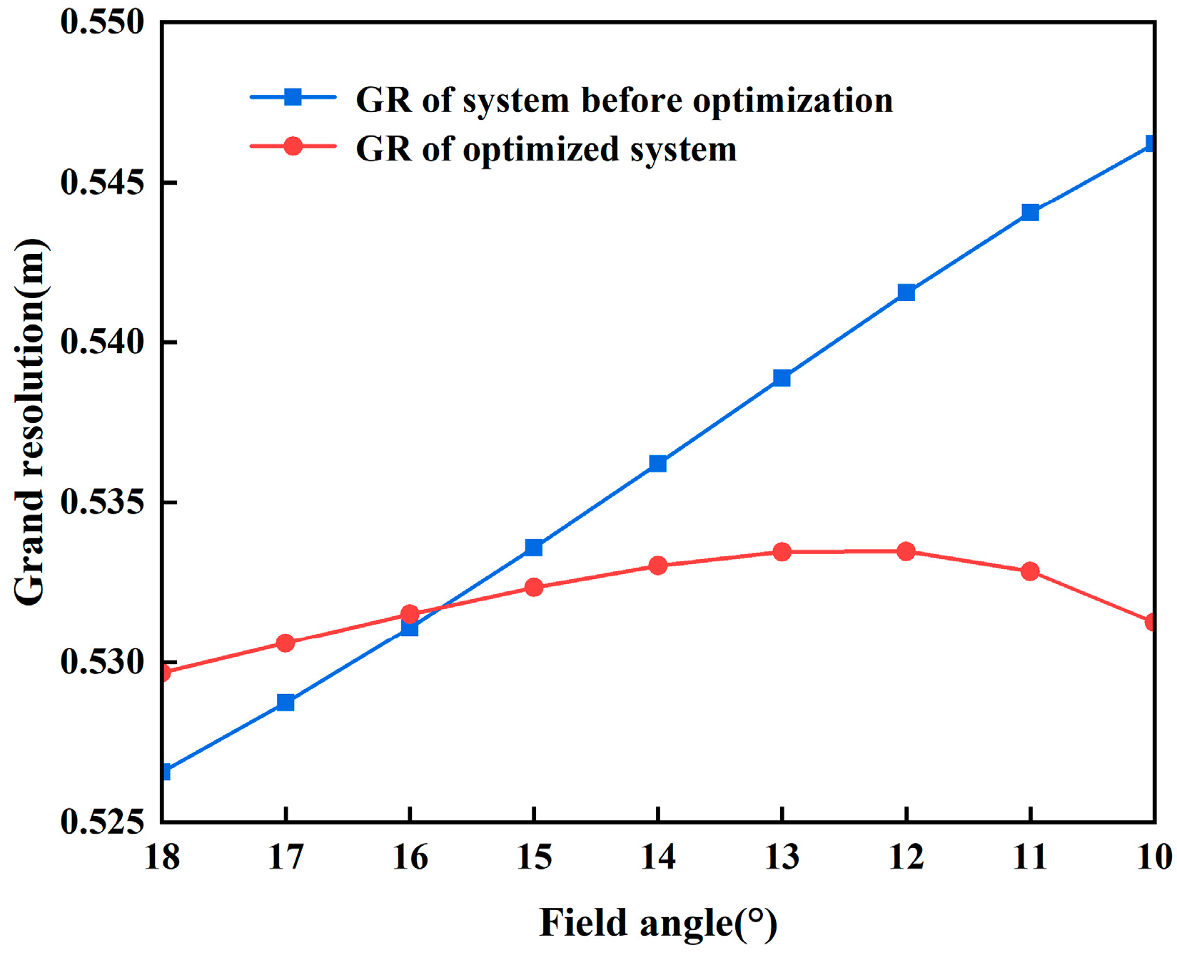
Figure 13 presents a comparative analysis of ground resolution (GR) performance, where the blue curve corresponds to the uncontrolled optical system and the red curve demonstrates the enhanced GR achieved through active light control implementation. The experimental results demonstrated significant GR stabilization through light control implementation. Prior to optical optimization, the system exhibited GR variations between 0.546 m and 0.527 m (ΔGR = 0.019 m). Following active light control implementation, the GR variation was substantially reduced to a narrow range of 0.528–0.531 m (ΔGR = 0.003 m), representing an 84.2% improvement in spatial resolution consistency. Comparative analysis of the optical performance curves indicated that the light-controlled system (red curve) achieved significantly improved GR uniformity, demonstrating an 80.4% reduction in ground resolution variation compared to the uncontrolled baseline (blue curve). This enhancement corresponded to a decrease in GR standard deviation from to across the entire field of view.

Figure 13.
Ground resolution at different field-of-view angles.
The optimized tilted imaging system achieved enhanced ground resolution (GR) uniformity through precise control of the field-of-view focal length (FFL) function during the optical design phase. This study conclusively demonstrated that the field-of-view focal length (FFL) parameter serves dual functions: (1) as an analytical metric for evaluating ground resolution (GR) in tilted imaging systems, and (2) as a design optimization variable for enhancing GR uniformity in next-generation camera systems.
Compared with the existing UAV imaging system, the resolution of this system was relatively constant, the distortion was relatively low, the weight was basically the same, the number of lenses was low, the lens material will be chosen to be lightweight and will be designed to reduce weight, and the power consumption was basically the same.
5. Conclusions
To overcome the inherent limitations of conventional unmanned aerial imaging systems in ground-target reconnaissance applications, this paper introduced the innovative concept of field-of-view focal length (FFL)—a spatially variant focal length parameter—enabling continuous focal length modulation from zero to the maximum field angle. Computational ray-tracing of the field-of-view focal length (FFL) was implemented to achieve simultaneous optimization of focal length control and imaging aberration correction throughout the entire optical system. This research employed high-degree-of-freedom optical freeform surfaces, specifically utilizing XY polynomial representations for the tertiary mirror while maintaining conventional quadratic conic surfaces for the primary and secondary mirrors. This hybrid configuration significantly enhanced the system’s aberration correction performance. Post-optimization analysis demonstrated exceptional optical performance, with the system achieving MTF values above 0.4 at the Nyquist frequency (33.4 lp/mm) while maintaining RMS spot radii consistently below the diffraction-limited Airy disk radius across the entire field of view. The results confirmed that ray-tracing optimization of the field-of-view focal length (FFL) effectively minimized ground resolution (GR) variations across the entire field of view, achieving consistent compliance with the constant-GR design specification.
In the machining of freeform optical surfaces, Wu et al. employed a dual-surface design incorporating two large-aperture freeform elements [7]. While this approach may enhance optical performance, it substantially increases fabrication complexity and manufacturing challenges. In contrast, our proposed design utilized a single freeform surface with a reduced aperture, which achieved a favorable trade-off between performance and manufacturability. Although this configuration resulted in a marginal reduction in system resolution, it significantly alleviated machining difficulties, thereby improving feasibility for practical implementation and mass production.
The airborne optical system with constant ground resolution capability provided stable, high-precision remote sensing data for Earth observation through dynamic optical adjustment. It enabled reliable all-weather target recognition in security surveillance and enhanced automated defect screening efficiency for industrial inspection.
With technological advancements, deeper integration of this system with autonomous drones will further improve its adaptive imaging performance in complex environments. This breakthrough solution holds significant potential for applications, such as smart city management, precision agriculture, and infrastructure inspection.
The designed imaging system was intended to be applied to UAV tilted ground photography, which requires a guaranteed observation angle of 10°. In the application, the design only achieved equal ground resolution imaging for small undulating ground, and further research is needed to explore the equal ground resolution problem for large undulating ground. For example, when photographing a tall building, the top of the building can achieve equal ground resolution imaging, but it is difficult to achieve equal ground resolution imaging on the side of the building, and to solve this problem, it is necessary to add the zoom function in the optical system, which is a direction for later research work.
Author Contributions
Conceptualization, Z.Y. and L.Y.; data curation, S.G.; formal analysis, S.G. and Q.C.; funding acquisition, Z.Y. and L.G.; investigation, Z.Y. and Q.X.; methodology, Q.C. and L.Y.; project administration, Z.Y.; resources, Z.Y. and Q.X.; software, S.G. and Q.C.; supervision, Z.Y.; validation, Z.Y.; visualization, S.G. and B.W.; writing—original draft, Z.Y. and S.G.; writing—review and editing, B.W. and L.G. All authors have read and agreed to the published version of the manuscript.
Funding
This research was funded by the National Natural Science Foundation of China (No. 62201566), the Key Scientific Research Plan of the Education Department of Shaanxi (No. 23JY035), the Youth Innovation Team of Shaanxi Universities (No. K20220184), and the Natural Science Foundation of Shaanxi Province (No. 2024JC-YBMS-523).
Institutional Review Board Statement
Not applicable.
Informed Consent Statement
Not applicable.
Data Availability Statement
Data underlying the results presented in this paper are not publicly available at this time but may be obtained from the authors upon reasonable request.
Acknowledgments
The authors sincerely appreciate all financial and technical support.
Conflicts of Interest
Qiang Xu is affiliated with Hubei Huazhong changjiang OP Toelectronic Technoldgy CO., LTD, Xiaogan 432009, China; All authors confirm that there is no conflict of interest to declare.
References
- Stewart, W. Freeform Optics: Notes from the Revolution. Opt. Photonics News 2017, 28, 34–41. [Google Scholar]
- Yang, T.; Duan, J.; Cheng, D.; Wang, Y. Freeform imaging optical system design: Theories, development, and applications. Acta Opt. Sin. 2021, 41, 115–143. [Google Scholar]
- Rolland, J.P.; Davies, M.A.; Suleski, T.J.; Evans, C.; Bauer, A.; Lambropoulos, J.C.; Falaggis, K. Freeform optics for imaging. Optica 2021, 8, 161–176. [Google Scholar] [CrossRef]
- Thompson, K.P.; Rolland, J.P. Freeform optical surfaces: A revolution in imaging optical design. Opt. Photonics News 2012, 23, 30–35. [Google Scholar] [CrossRef]
- Wu, W.; Jin, G.; Zhu, J. Optical design of the freeform reflective imaging system with wide rectangular FOV and low F-number. Results Phys. 2019, 15, 102688. [Google Scholar] [CrossRef]
- Zhu, J.; Zhang, B.; Hou, W.; Bauer, A.; Rolland, J.P.; Jin, G. Design of an oblique camera based on a field-dependent parameter. Appl. Opt. 2019, 58, 5650–5655. [Google Scholar] [CrossRef] [PubMed]
- Wu, W.; Zhang, B. Freeform imaging system with a resolution that varies with the field angle in two dimensions. Opt. Express 2021, 29, 37354–37367. [Google Scholar] [CrossRef] [PubMed]
- Zhang, B.; Hou, W.; Jin, G.; Zhu, J. Simultaneous improvement of field-of-view and resolution in an imaging optical system. Opt. Express 2021, 29, 9346–9362. [Google Scholar] [CrossRef] [PubMed]
- Zhao, H.; Guo, L.; Mao, X.; Duan, Y.; Xue, X. Design method of freeform off-axis three-mirror reflective imaging systems. Appl. Opt. 2023, 62, 7852–7859. [Google Scholar] [CrossRef] [PubMed]
- Chen, L.; Liu, H.; Feng, Z. Design Method of Wide Angle Lens Based on Optimization of Local Focal Length through Ray Tracing. Acta Photonica Sin. 2024, 53, 98–106. [Google Scholar]
- Yang, C.; Chen, Y.; Yu, K.; Su, P.; Fan, R. Design of receiving optical system for multi-channel beam-split spaceborne lidar. J. Chang. Univ. Sci. Technol. 2021, 44, 7–12. [Google Scholar]
- Meng, Q.; Wang, H.; Liang, W.; Yan, Z.; Wang, B. Design of off-axis three-mirror systems with an ultrawide field of view based on an expansion process of surface freeform and field of view. Appl. Opt. 2019, 58, 609–615. [Google Scholar] [CrossRef] [PubMed]
- Kevin, T. Description of the third-order optical aberrations of near-circular pupil optical systems without symmetry. J. Opt. Soc. Am. A Opt. Image Sci. Vis. 2005, 22, 1389–1401. [Google Scholar]
- Thompson, K. Description of the third-order optical aberrations of near-circular pupil optical systems without symmetry: Errata. J. Opt. Soc. Am. A 2009, 26, 699. [Google Scholar] [CrossRef]
- Fuerschbach, K.; Rolland, J.P.; Thompson, K.P. Theory of aberration fields for general optical systems with freeform surfaces. Opt. Express 2014, 22, 26585–26606. [Google Scholar] [CrossRef] [PubMed]
- Su, J.-J.; Tien, C.-H.; Tsai, Y.-L.; Wu, C.-T. A skew freeform reflector design method for prescribed off-axis irradiance. Results Phys. 2019, 13, 102193. [Google Scholar] [CrossRef]
- Meng, Q.; Wang, H.; Yan, Z. Residual aberration correction method of the three-mirror anastigmat (TMA) system with a real exit pupil using freeform surface. Opt. Laser Technol. 2018, 106, 100–106. [Google Scholar] [CrossRef]
- Luo, Y.; Li, L.; Feng, Y.; Zhao, H.; Li, X.; Bai, Q. Design method for initial structure of freeform surface optical system. Acta Opt. Sin. 2021, 41, 228–234. [Google Scholar]

Disclaimer/Publisher’s Note: The statements, opinions and data contained in all publications are solely those of the individual author(s) and contributor(s) and not of MDPI and/or the editor(s). MDPI and/or the editor(s) disclaim responsibility for any injury to people or property resulting from any ideas, methods, instructions or products referred to in the content. |
© 2025 by the authors. Licensee MDPI, Basel, Switzerland. This article is an open access article distributed under the terms and conditions of the Creative Commons Attribution (CC BY) license (https://creativecommons.org/licenses/by/4.0/).