Abstract
White-light interferometry is essential for surface topography measurement in precision manufacturing, yet existing algorithms face challenges in accuracy, speed, and robustness. Motivated by the application of deep learning in optical metrology, this study presents a novel simulation-driven, end-to-end deep learning approach that significantly advances white-light interference topography reconstruction. Validation with 200 simulated interferograms shows strong agreement with reference measurements. The neural network processes interferograms in <0.4 s with <0.3% calculation error, demonstrating real-time capability and noise robustness. Using simulated and experimental data from trapezoidal gratings, the method achieves a reconstruction error of 47.12 nm (<λ/8, λ ≈ 550 nm), outperforming traditional techniques by 9.0%. These results confirm the method’s superior accuracy, speed, and reliability for industrial metrology applications.
1. Introduction
As an effective tool for surface profile analysis, white-light interferometry technology has become widely popularized and significantly advanced in industrial manufacturing, biomedicine and materials science [1,2,3,4]. There is a growing demand for diverse and adaptable topographic surface analysis in the measurement and characterization of high-tech components [5,6,7,8]. However, traditional methods for white-light interference topography reconstruction face challenges in practical applications. One key issue is the complexity of the data processing process. These methods typically involve intricate data processing and analysis, drawing on knowledge from various fields such as optical principles, digital signal processing, and numerical calculations [9,10]. Additionally, algorithm selection and parameter tuning require expertise and engineering knowledge [11,12]. Furthermore, in practical applications, surface reconstruction algorithms must be resilient to factors like noise and environmental interference [13,14]. Therefore, the exploration of new surface reconstruction methods that streamline data processing to enhance the accuracy and stability of surface reconstruction represents a crucial focus of current research.
In recent years, deep learning has emerged as a potent tool for addressing problems through data-driven learning [15]. This advanced machine learning technology, utilizing multi-layer artificial neural networks, has found widespread application in imaging science [16,17,18,19]. This foundation paves the way for the integration of deep learning technology into the realm of optical metrology, presenting new opportunities for development in the field. In contrast to traditional “physics-based” methods, deep learning in optical metrology follows a “data-driven” approach, offering alternative solutions with superior performance for numerous challenging problems [20,21,22]. For instance, applications of deep learning in holography [23] and fringe projection profilometry [18,24] have demonstrated the capability to analyze fringes and directly generate holographic reconstructions. While the computational burden of training on stripe datasets can be significant, deep learning holds great promise for surface reconstruction. Acknowledging that training deep learning models necessitates extensive high-quality datasets, simulation-driven deep learning methods have been introduced in the literature [25,26]. This approach leverages simulated data to facilitate model training, compensating for the scarcity of real-world datasets. Through data simulation, the training dataset can be effectively expanded, enhancing the generalization ability of the deep learning model and better aligning it with real-world scenarios. This methodology introduces novel ideas and solutions for addressing challenges with limited actual data, thereby broadening the scope for training deep neural network (DNN) models and their application in optical metrology. In the field of white-light interferometry, deep neural networks have been explored for various tasks including resolution enhancement [27,28], noise reduction [29], and slope error correction [25]. Among these, Zhu et al. [25] employed a deep learning network to compensate for slope errors in reconstructed profile data; however, their method is limited to post-processing correction. In contrast, our work aims to achieve end-to-end topography reconstruction directly from white-light interferograms. To date, no study has reported a DNN-based end-to-end solution for white-light interferometric topography reconstruction algorithms.
Inspired by the widespread application of convolutional neural networks in the field of imaging, this study aims to explore a novel white-light interference topography reconstruction method by utilizing a simulation-driven deep learning model. In this research, a DNN architecture was constructed and trained using a substantial dataset consisting of simulated interference fringe patterns and real topography patterns (multiple inputs and single output). The developed DNN is capable of predicting the surface topography profile of an object based solely on a series of measured interference fringe patterns. A quantitative comparison between the proposed method and the traditional surface reconstruction algorithms demonstrates significant improvements in reconstruction accuracy and noise resistance, with a relative error of less than 0.3% and a reconstruction speed enhancement of two orders of magnitude, completing the process in under 0.4 s. Through comprehensive experimental validation using standard trapezoidal gratings (TGF11, MikroMasch, Wetzlar, Germany), the proposed method demonstrates remarkable performance: achieving sub-wavelength reconstruction accuracy with a root-mean-square error (RMSE) of 47.12 nm, representing a 9.0% improvement over conventional frequency domain analyses. A key advantage of this approach is the consolidation of data preprocessing, topography reconstruction, postprocessing, and any intermediate data processing steps into a single mapping function. Consequently, the DNN model can deliver end-to-end output measurements without requiring knowledge of the imaging system’s physical parameters. This study presents a more effective solution for topography reconstruction using white-light interference technology.
2. Methods
2.1. General Framework
This study innovatively integrates white-light interferometry with DNN to establish a comprehensive framework for high-precision reconstruction analysis of sample surface topography. Specifically, we constructed a simulated interferometry framework, generating a series of interferograms by adjusting the parameters of the measured surface. These interferograms served as input to the DNN, which is trained using a loss function to accurately output the reconstructed surface profile. In this section, we describe in detail the principles of white-light interferometry, simulation architecture, generation of training datasets, and DNN training based on simulated data, as well as the network framework, laying a solid foundation for subsequent experiments and analysis.
2.2. White-Light Interferometry
White-light interferometry employs an interferometric optical path to generate interference fringes by converging the measurement light reflected from the test surface with the reference light reflected from a mirror. For each wavelength of monochromatic light, interference occurs, and the maximum interference intensity is achieved only when the optical path difference (OPD) between the two beams is nearly zero. The contrast of the interference fringes decreases rapidly as the OPD increases [4,9]. By accurately locating the zero OPD positions for various points on the test surface, the relative height information of each point can be obtained, thereby enabling three-dimensional reconstruction of the entire field of view. Leveraging the high sensitivity of interference fringes to surface height information, this technique achieves nanometer-level height detection.
The intensity distribution of the white-light interference signal can be modeled as a cosine signal modulated by a Gaussian function. As the scanning distance changes, the actual white-light interference intensity at a given point can be described by the following equation [1,3]:
where represents the envelope function of the white-light interference signal; ; is the coherence length of the Gaussian spectral source; is the central wavelength; is the position along the scanning direction where the envelope of the white-light interference signal reaches its peak; is the initial phase difference between the reference beam and the measurement beam; is the background light intensity; is the fringe contrast; and is the scanning position along the optical axis. In summary, white-light interferometry achieves nanometer-level height measurements through precise zero optical path difference positioning, and its signal model provides a theoretical basis for simulation studies.
2.3. Simulation Architecture
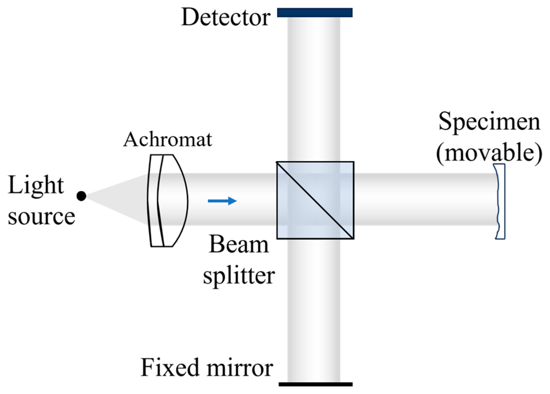
White-light interferometry is a robust technique for high-resolution surface profile measurements. By analyzing the interference pattern acquired in the optical path, precise surface profile measurements can be achieved. In this study, the optical simulation software Virtuallab Fusion (version 7.6.1) was utilized to construct the white-light interference optical path depicted in Figure 1 [30]. The white-light interferometry simulation model implements a Michelson interferometer configuration using a broadband xenon lamp source (400–700 nm spectral range) under controlled environmental conditions (20 °C, 101.33 kPa). An achromatic lens (#49-664, Edmund Optics, Barrington, IL, USA, 2° field of view, with optical parameters detailed in Table 1) [31,32] collimates the light before it encounters a 50:50 non-polarizing beam splitter. The reference arm incorporates a 50 × 50 mm ideal plane mirror with 100% reflectance across the operational spectrum, precisely positioned to maintain a 100 mm optical path length matched to the measurement arm. The measurement path terminates at a test sample modeled as a homogeneous high-reflectance medium with Lambertian scattering characteristics. Interference patterns are captured by a CCD detector featuring a 30 × 30 mm active window with 256 × 256 sampling points, positioned 100 mm from the beam splitter. The simulation accounts for the source’s short coherence length through adaptive step size control during numerical acquisition, enabling precise fringe pattern prediction. This simulated approach establishes a reliable foundation for subsequent experimental implementation.
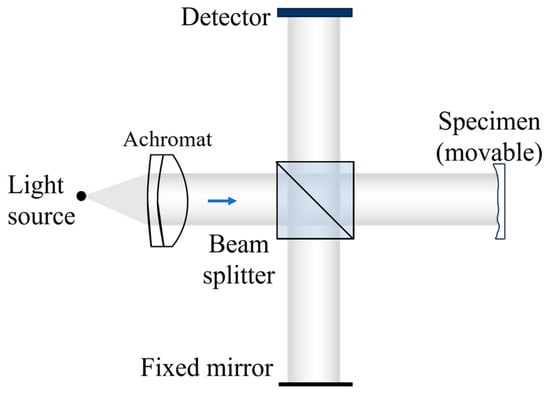
Figure 1.
Interference optical path diagram.

Table 1.
The configuration of the achromatic lens.
2.4. Generation of Training Datasets
In this study, a DNN is employed to process the measured interferogram for surface topography reconstruction. The performance of the DNN is directly influenced by the quality of the training dataset. To enhance the generalization capability of the DNN model, the training dataset in this research comprises interferograms from various surface types, encompassing a range of shapes and features, enabling the model to adapt to diverse measurement scenarios. Consequently, this study generated surfaces for measurement through simulation, including sinusoidal surfaces (sin(x)), 2Post surfaces, and step surfaces and utilized a white-light interference simulation model to create corresponding interferograms. The moving step size of the measured surface was set to 75 nm. For each surface, 200 interferograms were generated. By leveraging the 200 interferograms for each measured surface, the surface profile can be derived. In essence, for the DNN model, 200 inputs correspond to one output.
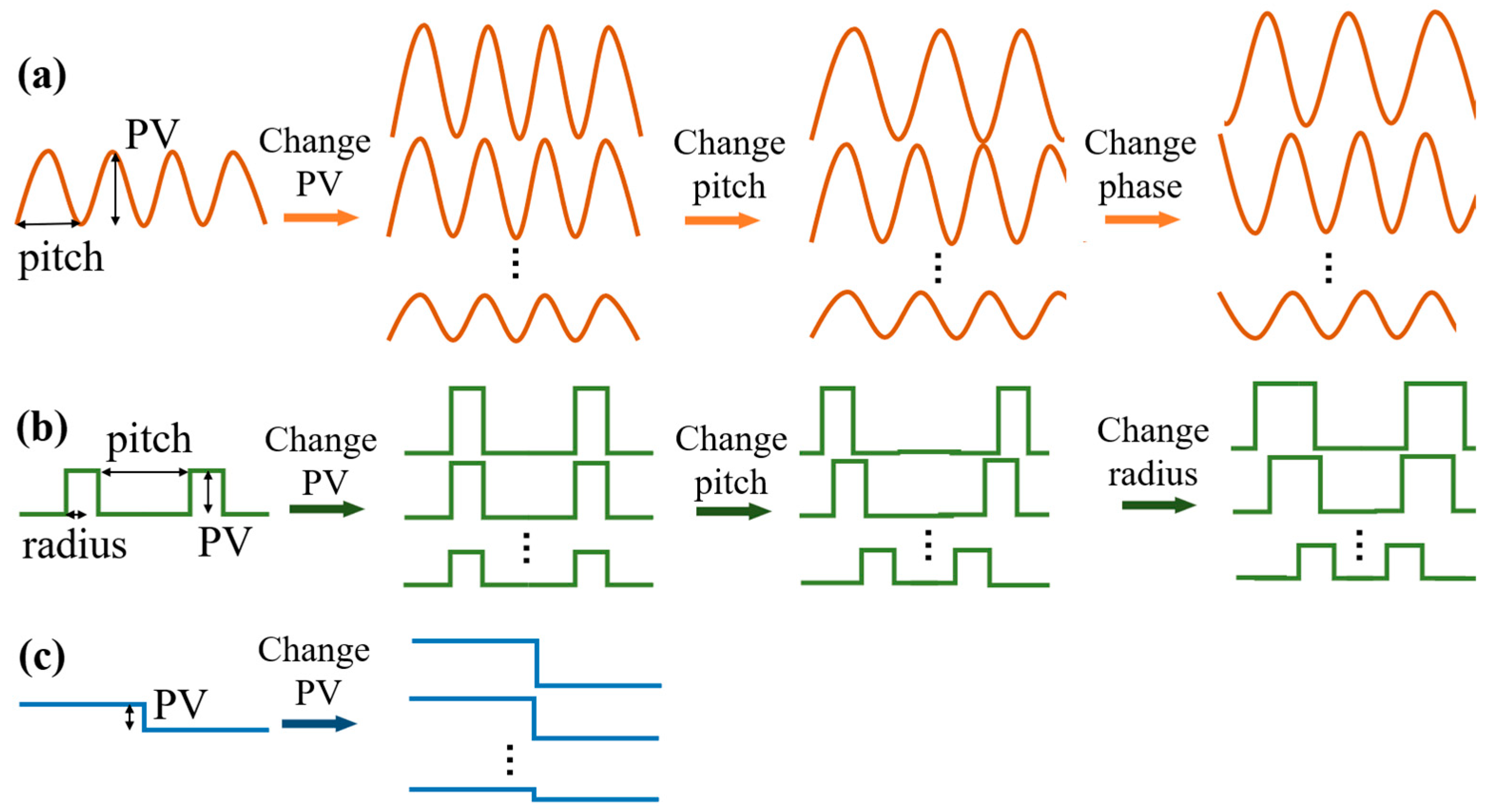
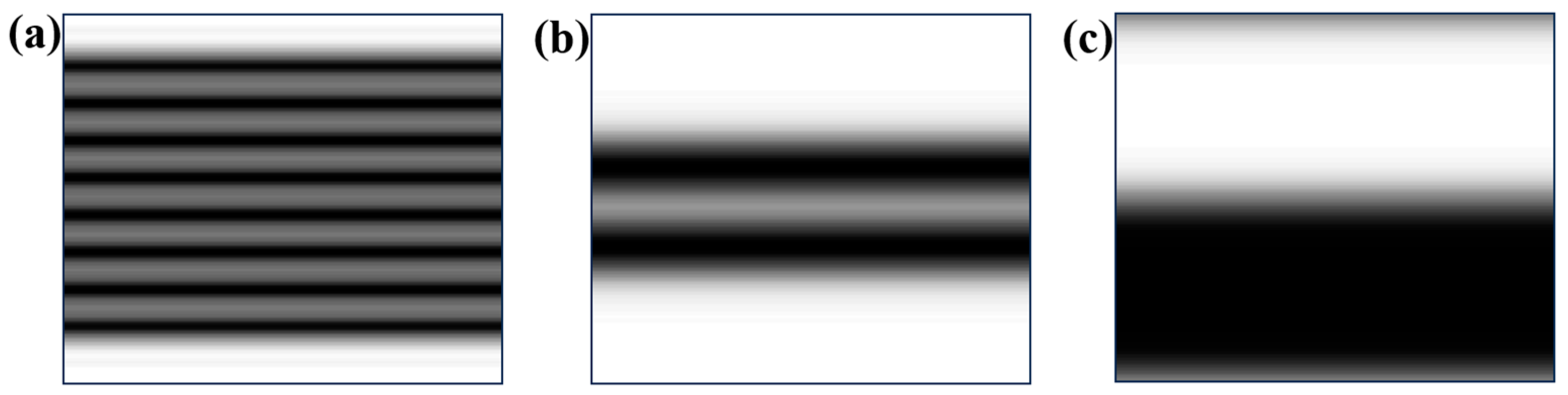
The generation process of the training dataset is shown in Figure 2. In schematic diagrams, contours are used to illustrate the geometric features of the surface being measured. PV denotes the peak-to-valley height, representing the maximum vertical deviation of the surface profile. The simulated dataset comprises 2100 surfaces equally divided into three types (700 per type). For sinusoidal surfaces, a series of sinusoidal surfaces are generated by varying the PV, pitch, and phase values (PV∈[0.05, 0.5] μm, pitch∈[5, 10] μm, and phase∈[0, 2π] rad). For 2Posts, different 2Posts are generated by changing the height, spacing, and radius (PV∈[0.1, 1] μm, radius∈[0.5, 10] μm, and pitch ∈[0.1, 10] μm). For steps, a series of height step surfaces are generated by varying the step height (PV∈[0.01, 1] μm). Parameters are randomized across 700 instances per type to ensure broad coverage of microstructural geometries. Figure 3 illustrates the simulated interferograms for sin(x), 2Posts, and step surfaces. Through such a training dataset generation method, it can be ensured that the DNN model can accurately reconstruct and predict when facing different types of surface topography.

Figure 2.
Generation of the training datasets. (a) sin(x); (b) 2Posts; (c) steps.
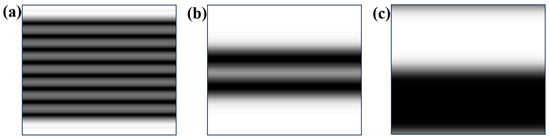
Figure 3.
Interferograms: (a) sin(x); (b) 2Posts; (c) step.
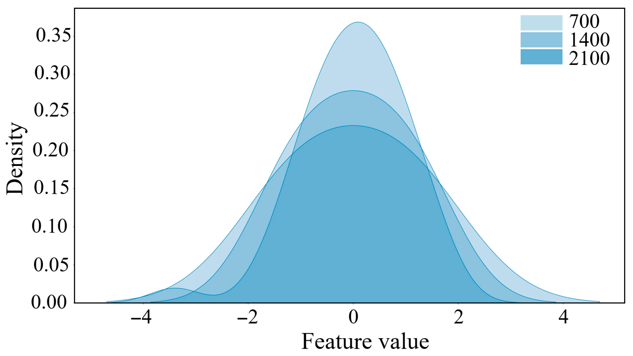
To determine the optimal training dataset size, a data distribution analysis is performed. Figure 4 presents kernel density estimates for datasets of 700, 1400, and 2100 simulated surfaces. Each dataset exhibits a unique mean and standard deviation. The 2100-surface dataset displays the highest peak density, indicating a tightly clustered distribution centered around the mean, with a low standard deviation. The 1400-surface dataset shows a slightly lower peak and a moderately increased standard deviation, suggesting greater data dispersion. Conversely, the 700-surface dataset exhibits the lowest peak and the widest spread, indicating the highest dispersion. The superior concentration of the 2100-surface dataset around its mean suggests a more consistent trend, allowing the model to better capture underlying data patterns and mitigate the effects of noise and outliers. Therefore, we selected a 2100-surface dataset for training, as it provides a more accurate representation of the underlying data characteristics.

Figure 4.
Kernel density distribution curves of three data quantities.
This comprehensive dataset not only helps improve the model’s generalization ability but also allows for a better understanding and interpretation of the model’s reconstruction results. In future research, the dataset will be further expanded and the characteristics of more different types of surfaces will be explored to further improve the performance and scope of use of the DNN model.
2.5. DNN Training Based on Simulation Data
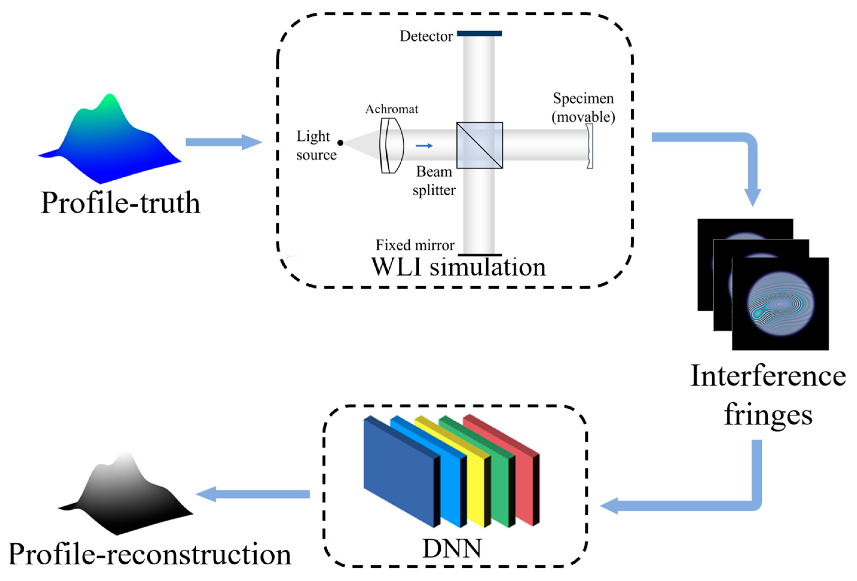
Considering that it is difficult to obtain the real surface condition in practical applications, this study employs the simulated ground truth surface generated by simulation without collecting a real measurement dataset. This is the advantage of such simulation-driven machine learning methods. Figure 5 illustrates the process of simulated data-driven deep learning in detail. Firstly, the ground truth profile T(x,y) and interferogram (x,y)(i = 1, 2, 3 … 200) are generated by white-light interferometer simulation. Secondly, the obtained (x,y) are used as the model input to train the DNN model. The output of the DNN model is the reconstructed topography R(x,y). The employed DNN structure is U-Net, a convolutional neural network with an encoder–decoder. As the output of DNN, R(x,y) can be described as a mapping function R:
where (i = 1, 2, 3 … 200) represents the input interferogram sequence (200 frames of 256 × 256 pixels).

Figure 5.
The training process of DNN.
In the reconstruction process, the loss function is utilized to assess the difference between the model output and the actual measured surface profile. The calculation formula for this is as follows:
By minimizing this difference, the optimal weights and mapping relationship can be determined, enabling the model to accurately reconstruct the corresponding surface from the input interferogram. As a result, the reconstruction challenge transforms into an optimization problem. During the optimization process, the Adam adaptive learning rate method is employed to adjust the update step size and method of the weight parameters according to the gradient information and historical update status. This approach accelerates convergence and prevents the model from getting stuck in local optimal solutions. Through the iterative optimization and continuous adjustment of weight and mapping relationships, the model progressively learns the intricate mapping between input interference fringes and output reconstruction surfaces, facilitating precise reconstruction. A total of 80% of the dataset was used as the training set to train the model and 20% as the test set. The error on the test set is used as the generalization error of the final model in dealing with real-world scenarios. During training, the Adam optimizer is used with the learning rate set to 10−5, and other parameters are default parameters, namely beta_1 = 0.9, beta_2 = 0.999, epsilon = 10−8 to optimize the network parameters. As shown in Equation (2), the U-Net is trained using the mean squared error (MSE) as the loss function to train U-Net. The batch size is set to 1 and the number of epochs to 5. The training time is 8 h 24 min. The implementation is performed using Python (version 3.7) and the PyTorch framework (version 1.9.0) on a computer equipped with Intel Core i7-10700k CPU, 48GB RAM (Intel, Santa Clara, CA, USA), and NVIDIA GeForce RTX 4090 GPU (NVIDIA, Santa Clara, CA, USA). This deep learning methodology, rooted in simulated data, presents a novel solution for optical measurement. By integrating simulation technology with deep learning algorithms, efficient surface topography reconstruction can be achieved without real data, offering a more convenient and reliable solution for practical applications.
2.6. Network Architecture
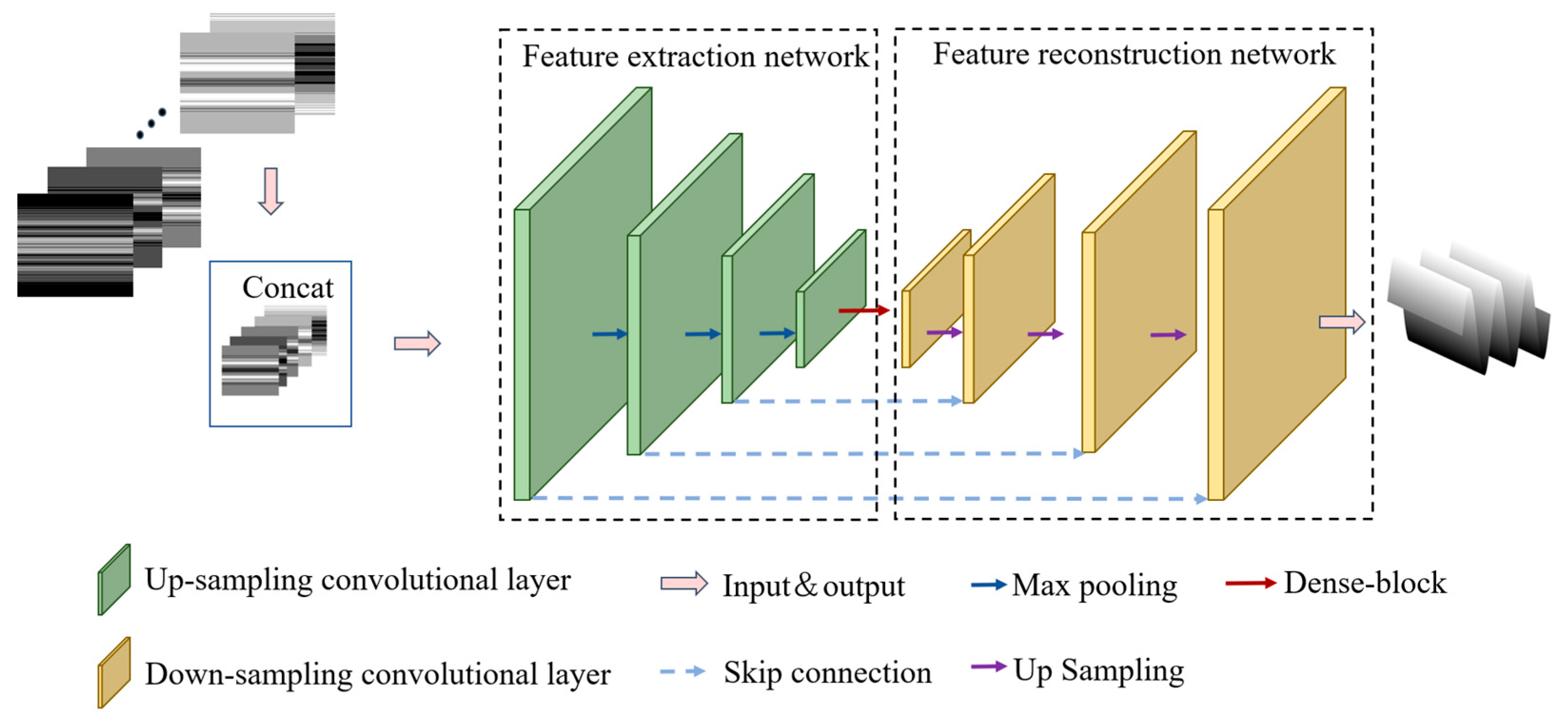
A series of interference fringe images with varying optical path differences are collected, which are generated by white-light interference optical simulation. To obtain the final reconstructed images, these images are concatenated and input into the U-Net network for processing. U-Net is a convolutional neural network, which is primarily used for image segmentation and complex tasks [33,34]. The network inherently captures temporal correlations in interferogram sequences through 3D convolutional operations that jointly process spatial and temporal dimensions (x, y, t), where the temporal kernel (size = 3) detects frame-to-frame intensity variations characteristic of white-light interference. The architecture of the U-Net network is shown in Figure 6, which includes a feature extraction network and a feature reconstruction network, and uses skip connections to convey contextual information [35]. In contour reconstruction, 200 concatenated white-light interferogram images of size 256 × 256 are input into the feature extraction network of U-Net. The network includes a series of convolution and pooling layers designed to extract texture details, edge features, optical path information, and spatial characteristics from the input image. The output feature maps of the feature extraction network are connected to the corresponding layers of the feature reconstruction network through skip connections. The feature extraction network gradually increases the size and channel count of the feature map through convolutional layers and max pooling functions and restores the image details and spatial information through deconvolution layers and convolution layers. The output feature maps of each stage of the feature extraction network are channel-concatenated with the upsampled feature maps output by the downsampled convolutional layer through skip connections to avoid losing additional information. The feature reconstruction network leverages contextual information transmitted by skip connections and combines features from different locations to enhance restoration of surface profile details and structure depth. Finally, a 1 × 1 convolutional layer is used for feature fusion, and the output is a surface contour of size 256 × 256. Through this approach, U-Net extracts features from a series of interference images and reconstructs a more precise and comprehensive surface contour image by combining feature information. This process effectively exploits the temporal coherence in white-light interferometry, where the network learns to weight phase information differently across the 200-frame sequence based on local contrast variations. To reduce the number of parameters, the kernel size of the convolutional layer is 3 × 3. Each convolutional layer is followed by a ReLU activation function for non-linear transformation, and a 2 × 2 max-pooling operation is used for downsampling with a stride of 2.

Figure 6.
The architecture of the U-Net.
3. Results and Discussion
3.1. Performance of DNN Reconstruction on Simulated Data
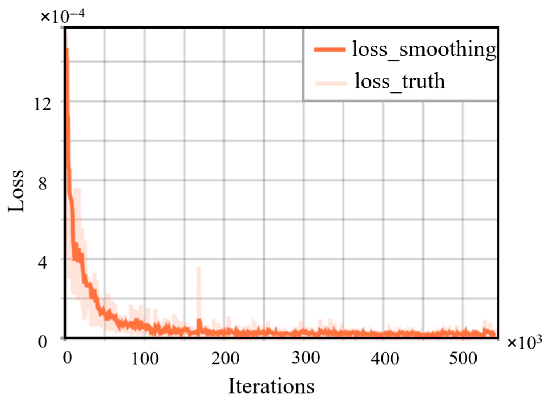
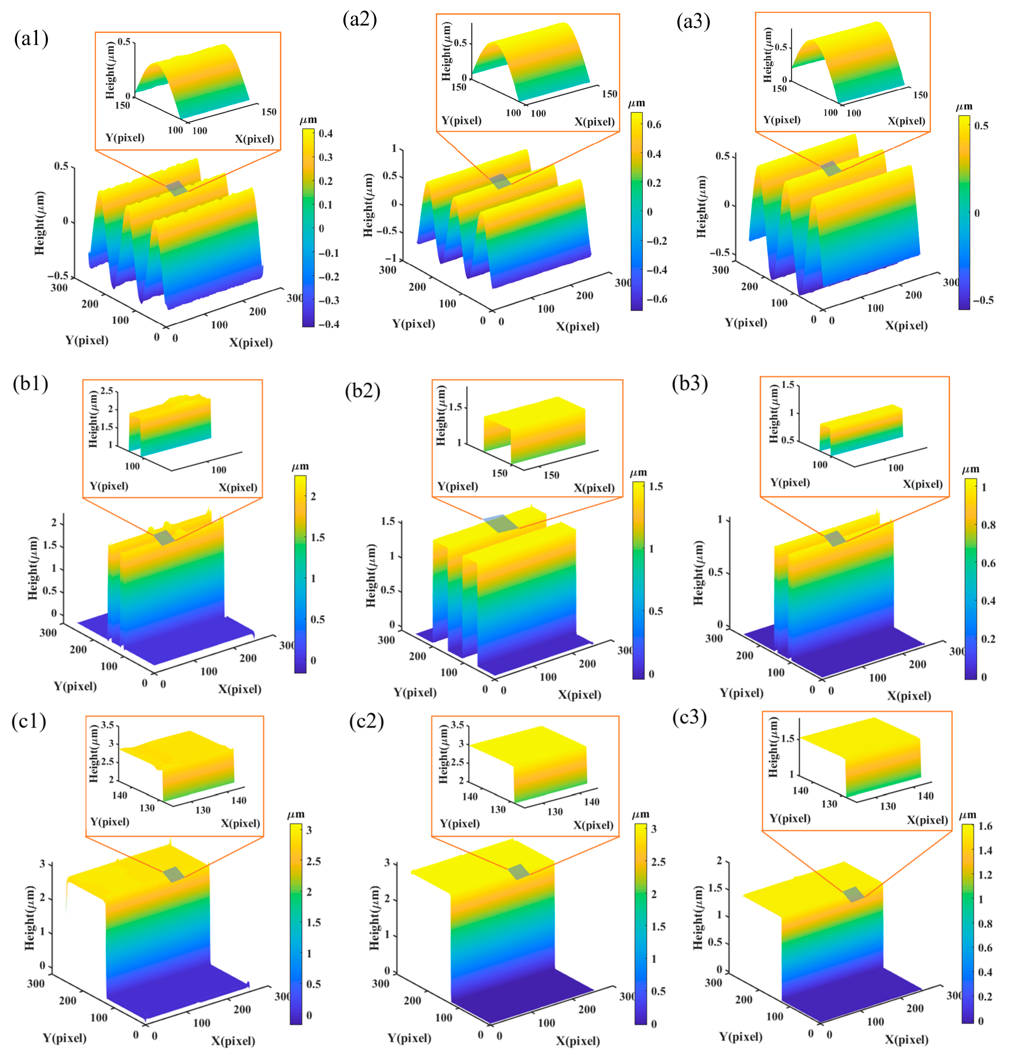
During the model training phase, a total of 1500 epochs were set, with each batch consisting of 2 samples. Additionally, the number of iterations was set to 1500, meaning that with each batch trained, the number of iterations increases by one. To enhance the readability of the graph, the actual loss curve was designated as the background, while the loss curve with a smoothing factor of 0.80 was set as the foreground. Figure 7 illustrates the evolution of the loss function throughout the model training process. From the results depicted in Figure 7, it is evident that the loss function gradually decreases and approaches a stable state as training progresses. Once the number of training iterations reaches 250,000, the change in the loss function becomes minimal, indicating that the model training is nearing convergence. Furthermore, the topography of 300 surface samples, including sinusoidal surfaces, 2Posts, and steps, from the test set was reconstructed. During the model training, random testing processes were employed. Figure 8 shows the results of random testing at epochs 100, 800, and 1500. It can be observed that as the number of epochs increases, the surface reconstruction output of the model becomes smoother and more accurate. This trend indicates that as training progresses, the model’s performance improves gradually, enabling it to better capture the topographical characteristics of the input data and generate more precise reconstruction results.

Figure 7.
The loss curve changes during model training.
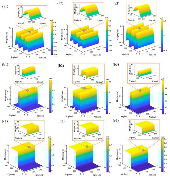
Figure 8.
Random test results during the model training process. (a1,b1,c1) Model output at epoch = 100; (a2,b2,c2) model output at epoch = 800; (a3,b3,c3) model output at epoch = 1500.
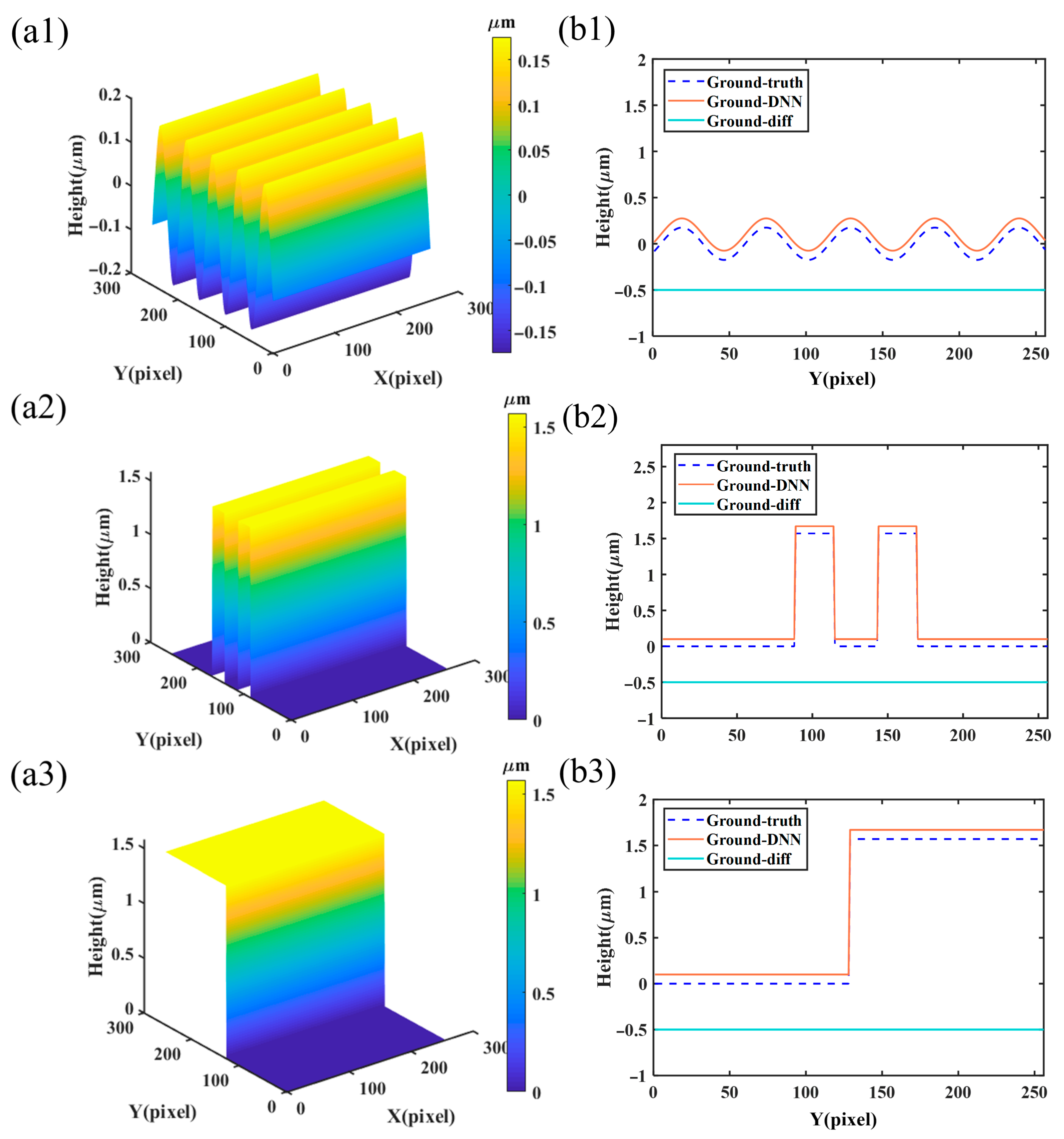
To quantitatively evaluate the surface reconstruction ability of DNN, the Michelson white-light interference model was utilized to measure sin(x), 2Posts, and step surface and generate corresponding interference patterns. The real parameter data of the measured surface is presented in Table 2, with the surface topography depicted in Figure 9a1–a3, respectively. The profiles at x = 0 were compared, as illustrated in Figure 9b1–b3 (the differences between the DNN reconstructed contours and the true contours are adjusted for display purposes). The results indicate a high level of consistency between the reconstructed surface topography profile and the real surface profile. The average height deviations between the reconstructed profiles output by the DNN and the real surface profiles are 0.039 nm, 0.054 nm, and 0.061 nm, respectively, with relative errors below 0.3%. This demonstrates the proficient performance of the DNN in surface topography reconstruction, accurately capturing the details and structures of various surface types.
Table 2.
Topographical parameters of the measured surface.

Figure 9.
Performance of the DNN on simulated data. (a1–a3) Real topography images of the measured surface; (b1–b3) real topography contours, DNN reconstructed topography contours, and the differences between the reconstructed and real topography contours.
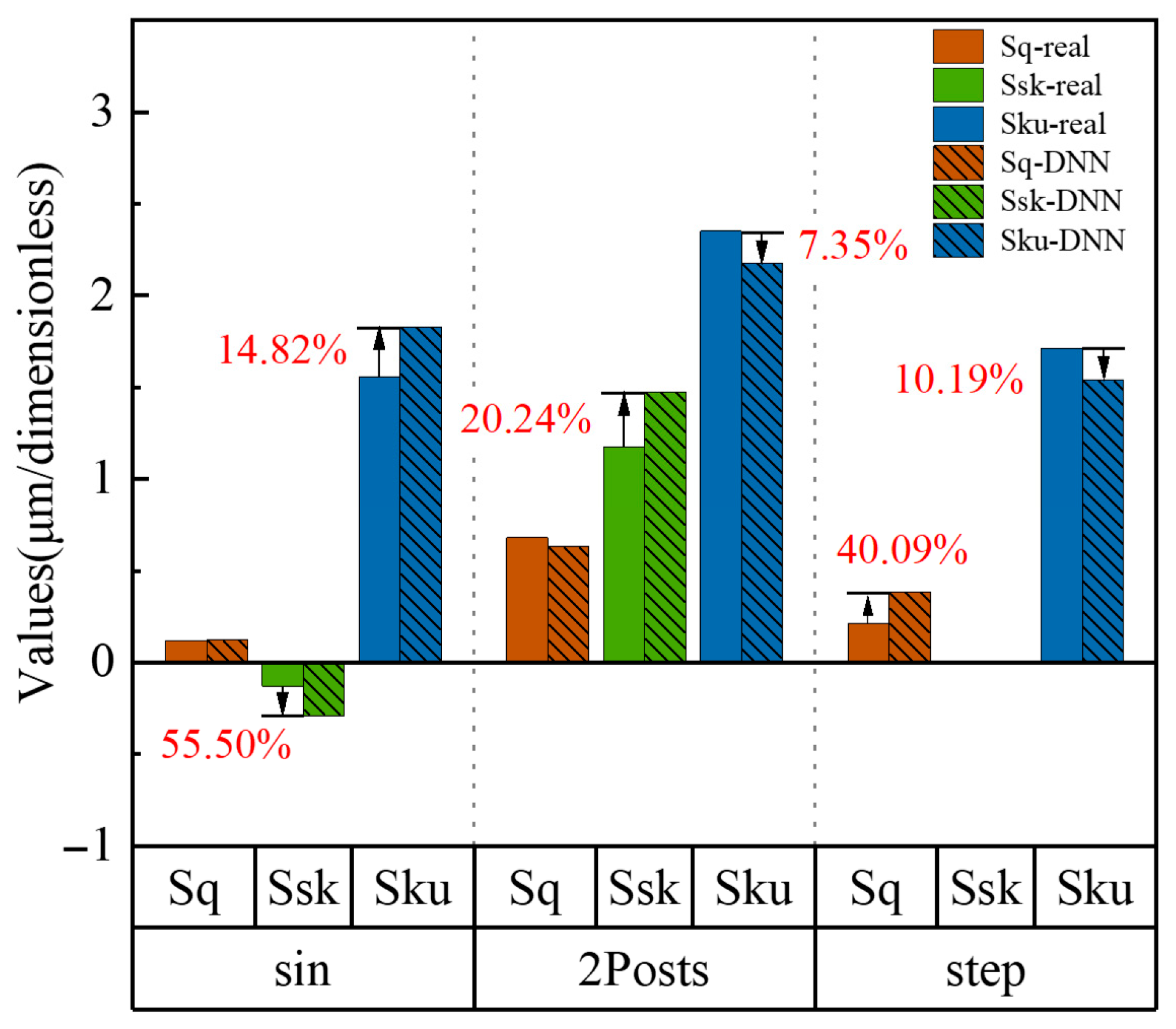
Figure 10 presents a comparative analysis of the topography characteristics of the DNN-reconstructed and real measured surfaces in terms of Sq, Ssk, and Sku parameters. While the Sq parameter shows acceptable deviations for sin and 2Posts surfaces, the DNN-reconstructed Sq value is elevated for the step surface. This might be attributed to overfitting of the model to subtle textural features, resulting in inaccurate quantification. Significant deviations are observed in the Ssk parameter for the sin surface, potentially due to insufficient representation of the highly asymmetric distribution of sin in the training data, hindering accurate reconstruction. For all three surfaces, the deviations in the Sku parameter remain within 15%, considered acceptable. Overall, the DNN method effectively reconstructs topography parameters across various scenarios, exhibiting high accuracy, particularly for complex surfaces, thus validating its efficacy. However, the observed discrepancies highlight avenues for model improvement. Optimizing the training data and model architecture promises further enhancements in reconstruction accuracy.

Figure 10.
Sq, Ssk, and Sku parameters: comparative analysis of characterization parameters of DNN reconstructed surface and real measured surface. (For the step surface’s Ssk parameter, both the real measured surface value (0.000035) and the DNN-reconstructed surface value (0.000029) are too small for clear visualization in the bar chart.)
3.2. Performance of DNN Reconstruction on Experimental Data
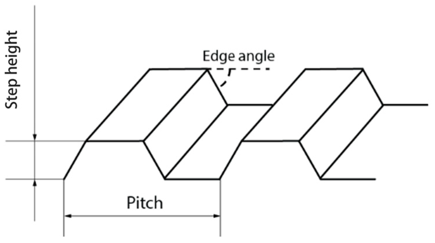
To validate the reconstruction performance of the proposed model on actual grating devices, we parametrically generated 100 additional trapezoidal surface training samples based on the geometric characteristics of laboratory-available trapezoidal gratings for specialized network training. As illustrated in Figure 11, diverse samples were created by systematically varying three geometric parameters (step height, pitch, and edge angle), with corresponding interferograms simulated using a white-light interference model to construct the training dataset.
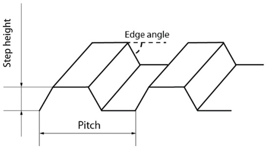
Figure 11.
Schematic diagram of trapezoidal surface.
The interferometric measurement system (Figure 1) employed a supercontinuum light source (NKT Photonics, EXR-15, 400–700 nm, Copenhagen, Denmark) for broadband illumination. A beam splitter (50:50 ratio) divided the light into reference and measurement arms. Sample displacement was achieved through nanometer-scale scanning using a piezoelectric transducer (Coremorrow, P66.X30-C1, Harbin, China), with interference patterns captured by an industrial camera (HIKROBOT, MV-CA013-A0UC, Hangzhou, China).
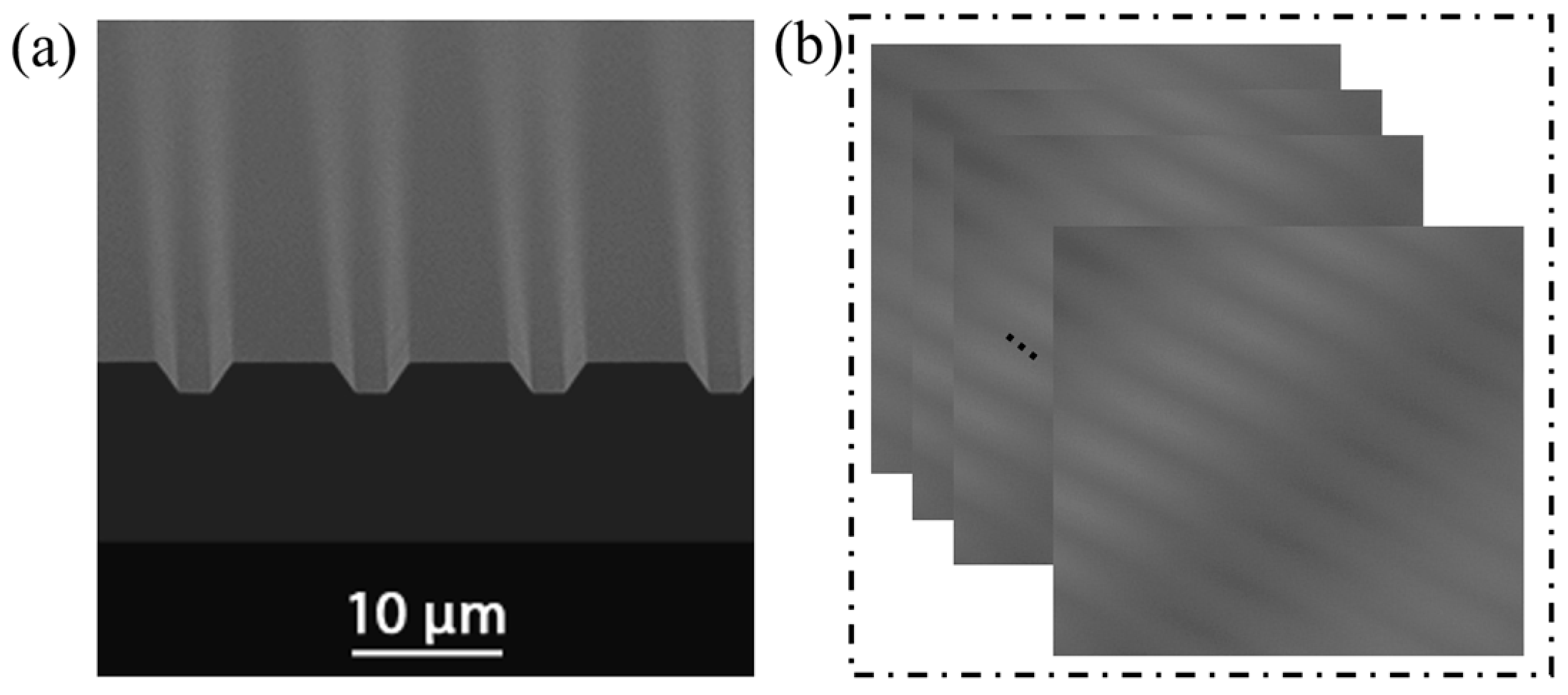
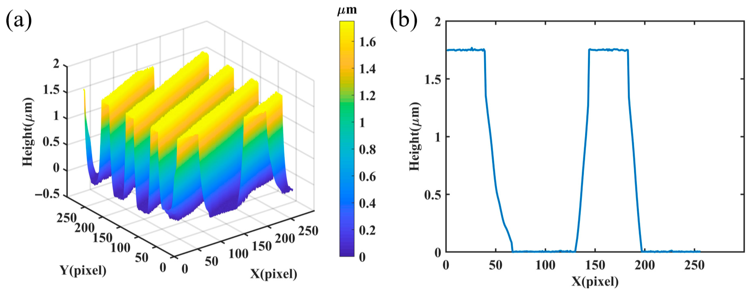
To evaluate the generalization capability of our DNN method in untrained CSI measurements, we tested a standard trapezoidal grating (MikroMasch, TGF11, Wetzlar, Germany; step height: 1.75 μm, pitch: 10 μm, edge angle: 54.74°) as the sample. The SEM image in Figure 12a confirms the sample’s geometry, while Figure 12b shows 200 acquired interferograms serving as DNN inputs. The DNN successfully reconstructed the 3D topography (Figure 13a), exhibiting clear periodic step structures with height distributions (0–1.75 μm) matching expected geometric parameters. The cross-sectional profile at pixel X = 200 (Figure 13b) demonstrates characteristic trapezoidal features, verifying single-pixel reconstruction accuracy. As quantified in Table 3, the proposed DNN achieved superior performance (RMSE: 47.12 nm) compared to conventional methods: the centroid (58.24 nm) and Hilbert transform (64.33 nm) methods showed higher errors due to fringe contrast sensitivity. Fourier transform (FT) (59.13 nm) and spatial frequency domain analysis (FDA) (51.80 nm) exhibited improved but still inferior performance. The DNN’s 9.0% RMSE reduction versus the best conventional method (FDA) demonstrates enhanced noise immunity and generalization. The sub-wavelength accuracy (47.12 nm < λ/8, λ ≈ 550 nm) confirms the method’s capability for high-precision micro/nano-structure metrology, surpassing the λ/4 theoretical limit of conventional interferometry.
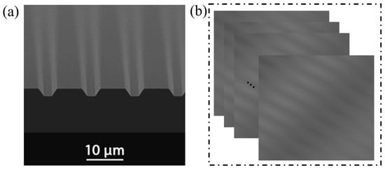
Figure 12.
(a) SEM image of the TGF grating. (b) Interferograms of experimentally measured gratings.

Figure 13.
The reconstruction results of grating by DNN method: (a) 3D surface of the measured grating output by the DNN; (b) height profile at pixel X = 200.
Table 3.
Comparison of the reconstruction accuracy of the centroid, Hilbert transform, FT, FDA, and proposed DNN methods.
3.3. Noise Resistance Performance
During the actual white-light interference topography measurement process, shot noise may be present in the interference pattern due to light source instability, stray light in the optical path, and surface roughness of optical components [36]. This noise manifests as random bright or dark spots in the image, which can introduce instability in the reconstruction results [37]. Investigating the noise resistance performance of surface reconstruction algorithms is crucial to ensure the accuracy of reconstructed surfaces in practical applications. The utilization of upsampling, downsampling structures, and skip connections in the U-Net model employed in this study aids in mitigating the impact of noise and preserving the accuracy of surface reconstructions.
The noise can be estimated as follows [38,39]:
where in the Cartesian coordinate system, is a weighting factor in the range [0,1], is a uniform distribution of random numbers in [−1,1], and is a 3D interference image. In white-light interference scanning measurements, the noise value is typically less than 10% of the signal [40], corresponding to . Therefore, the interferogram after adding noise is
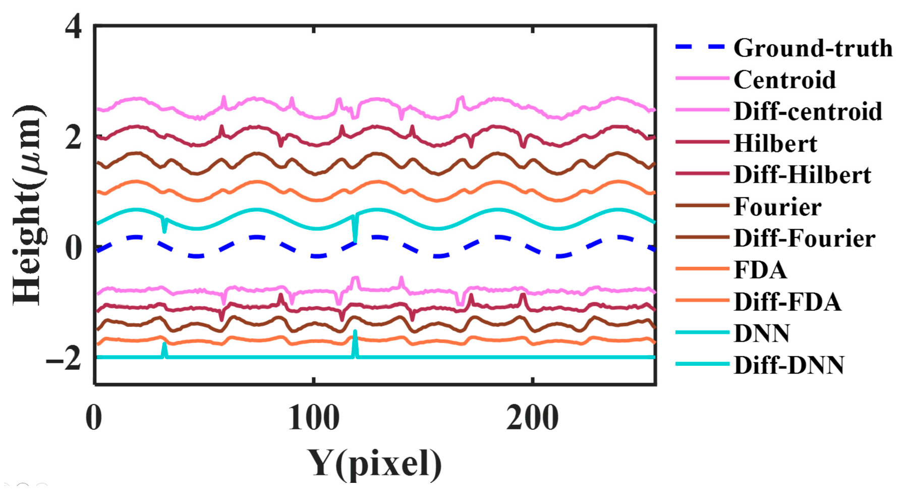
To evaluate the performance of the proposed method in terms of noise resistance, interference images with scattered noise were used as inputs for surface reconstruction. By controlling the level of scattered noise, the performance of the DNN model under different noise conditions was assessed. A sinusoidal surface was measured as the target surface, and the contour at x = 100 was selected for quantitative comparison. Ground-truth represents the actual contour of the target surface (PV is 0.37 μm, pitch is 6.5 μm), Ground-DNN represents the reconstructed contour by the DNN, and Ground-diff-DNN represents the difference between the reconstructed contour and the actual contour. It can be observed from Figure 14 that the increase in scattered noise has little impact on the accuracy of the contour reconstructed by the DNN method, with only a small amount of burrs phenomena. In contrast, the reconstructed contours of the centroid [41], Hilbert transform [42], FT [9,43,44], and FDA [45] methods exhibit deformation and are significantly affected by noise, leading to a noticeable decrease in reconstruction accuracy. In the comparative analysis in Table 4, the measurement accuracy of the centroid, Hilbert transform, FT, and FDA methods decreases with increasing noise levels, while the measurement accuracy of the DNN reconstruction method remains relatively stable. When the noise level is = 0.1, the RMSE of the reconstructed contour using the DNN method is only 43.89 nm. Therefore, the proposed surface reconstruction method demonstrates superior noise resistance compared to traditional methods, which is of great significance for achieving high-precision surface reconstruction and widespread practical engineering applications.
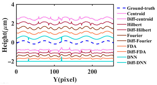
Figure 14.
Comparison of the noise resistance performance among the centroid, Hilbert transform, FT, FDA, and proposed DNN methods (using sin surface as an example, = 0.05).
Table 4.
Noise resistance performance analysis of the centroid, Hilbert transform, FT, FDA, and proposed DNN methods.
3.4. Computational Efficiency
In practical measurement applications, computational efficiency is crucial for the shape reconstruction of a large number of interferograms [46]. The trained U-Net model utilizes an encoder–decoder structure, effectively extracting multi-scale features while preserving spatial details through hierarchical fusion [47]. To quantitatively analyze the computational efficiency of the DNN reconstruction algorithm, interference fringe datasets of sinusoidal surface, 2Posts, and step surfaces were used to evaluate different surface reconstruction algorithms. By comparing the computational performance of the proposed surface reconstruction method with the centroid, Hilbert transform, FT, and FDA methods, differences in their computational efficiency can be observed, as detailed in Table 5. The timing results were obtained using CPU implementations (Intel Core i7-10700K) to ensure fair comparison with conventional algorithms. Quantitative comparison results demonstrate that the DNN model can complete surface reconstruction in < 0.4 s, delivering 4–40× speedup over traditional methods. Therefore, the proposed surface reconstruction method exhibits efficient computational performance, facilitating online surface inspection in white-light interference, and offering a faster and more accurate solution for surface reconstruction in the field of optical measurement.
Table 5.
Computational efficiency comparison among the centroid, Hilbert transform, FT, FDA, and proposed DNN methods.
4. Conclusions
This study presents a groundbreaking simulation-driven deep learning approach that enables direct, high-fidelity surface reconstruction from white-light interferograms, bypassing traditional complex processing pipelines. Our method establishes three significant advances in optical metrology: (1) unprecedented processing speed (<0.4 s per reconstruction), achieving a 40× acceleration over conventional algorithms while maintaining sub-wavelength accuracy (47.12 nm RMSE, λ/8); (2) superior noise robustness, with <0.3% error under realistic noise conditions (up to 10% intensity variation); and (3) generalized performance across diverse surface topologies, as demonstrated through rigorous validation on sinusoidal, 2Posts, step surfaces, and trapezoidal gratings (9% accuracy improvement over a Fourier-domain analysis). The framework’s <0.4 s processing capability and noise resilience also suggest potential applicability to ultrafast laser interferometry (femtosecond/picosecond regimes), pending adaptation for nonlinear interference modeling. While the current implementation shows robust performance for typical industrial surfaces, performance may degrade for highly rough/tilted surfaces or transparent films—a limitation that will be addressed through future extensions combining hybrid physical–deep learning models. The framework’s modular design permits seamless performance expansion through targeted retraining with new data types. These results position our method as a promising solution for industrial optical metrology, particularly in online white-light interferometry applications where both precision and speed are critical. The framework’s architecture also shows potential for extension to ultrafast measurement scenarios in future work.
Author Contributions
X.Q.: Conceptualization, Investigation, Methodology, Data curation, Formal analysis, Validation, Visualization, Writing—original draft. Y.L.: Writing—review and editing, Resources, Funding acquisition, Supervision, Project administration. Y.W.: Supervision, Funding acquisition. Z.L.: Supervision, Funding acquisition. All authors have read and agreed to the published version of the manuscript.
Funding
This study was financially supported by the National Natural Science Foundation of China (No. 61905062, 61927815) and the China Postdoctoral Science Foundation (No. 2020M670613).
Institutional Review Board Statement
Not applicable.
Informed Consent Statement
Not applicable.
Data Availability Statement
The data will be made available on request.
Conflicts of Interest
The authors declare no conflicts of interest.
References
- Ma, L.; Jia, J.; Pei, X.; Sun, F.-M.; Zhou, H.; Li, J.-Q. A robust surface recover algorithm based on random phase noise correction for white light interferometry. Opt. Lasers Eng. 2020, 128, 106016. [Google Scholar] [CrossRef]
- Feng, X.; Senin, N.; Su, R.; Ramasamy, S.; Leach, R. Optical measurement of surface topographies with transparent coatings. Opt. Lasers Eng. 2019, 121, 261–270. [Google Scholar] [CrossRef]
- Zhang, Z.; Chen, J.; Yang, H.; Yin, Z. Accurate Measurements of Droplet Volume With Coherence Scanning Interferometry. IEEE Trans. Instrum. Meas. 2023, 72, 1–15. [Google Scholar] [CrossRef]
- Dong, Y.; Li, Z.; Zhu, L.; Zhang, X. Topography measurement and reconstruction of inner surfaces based on white light interference. Measurement 2021, 186, 110199. [Google Scholar] [CrossRef]
- Wu, X.; Zhu, L.; Fang, F.; Zhang, X. Research on the quality control technology of micro-topography machining based on in situ white light interferometry. Measurement 2023, 220, 113257. [Google Scholar] [CrossRef]
- Lu, Y.; Park, J.; Yu, L.; Kim, S.-W. 3D profiling of rough silicon carbide surfaces by coherence scanning interferometry using a femtosecond laser. Appl. Opt. 2018, 57, 2584–2589. [Google Scholar] [CrossRef]
- Zou, Y.; Li, Y.; Kaestner, M.; Reithmeier, E. Low-coherence interferometry based roughness measurement on turbine blade surfaces using wavelet analysis. Opt. Lasers Eng. 2016, 82, 113–121. [Google Scholar] [CrossRef]
- Liu, M.; Fai Cheung, C.; Senin, N.; Wang, S.; Su, R.; Leach, R. On-machine surface defect detection using light scattering and deep learning. J. Opt. Soc. Am. A 2020, 37, B53–B59. [Google Scholar] [CrossRef]
- Wu, D.; Fang, F. Development of surface reconstruction algorithms for optical interferometric measurement. Front. Mech. Eng. 2021, 16, 1–31. [Google Scholar] [CrossRef]
- Su, R.; Coupland, J.; Sheppard, C.; Leach, R. Scattering and three-dimensional imaging in surface topography measuring interference microscopy. J. Opt. Soc. Am. A 2021, 38, A27–A42. [Google Scholar] [CrossRef]
- Sun, Y.; Gao, Z.; Ma, J.; Zhou, J.; Xie, P.; Wang, L.; Lei, L.; Fu, Y.; Guo, Z.; Yuan, Q. Surface topography measurement of microstructures near the lateral resolution limit via coherence scanning interferometry. Opt. Lasers Eng. 2022, 152, 106949. [Google Scholar] [CrossRef]
- Cui, K.; Liu, Q.; Huang, X.; Zhang, H.; Li, L. Scanning error detection and compensation algorithm for white-light interferometry. Opt. Lasers Eng. 2022, 148, 106768. [Google Scholar] [CrossRef]
- Teale, C.; Barbastathis, G.; Schmidt, M.A. Vibration Compensated, Scanning White Light Interferometer for In Situ Depth Measurements in a Deep Reactive Ion Etcher. J. Microelectromechanical Syst. 2019, 28, 441–446. [Google Scholar] [CrossRef]
- Peter de, G.; Jack, D. Definition and evaluation of topography measurement noise in optical instruments. Opt. Eng. 2020, 59, 064110. [Google Scholar] [CrossRef]
- LeCun, Y.; Bengio, Y.; Hinton, G. Deep learning. Nature 2015, 521, 436–444. [Google Scholar] [CrossRef] [PubMed]
- Rivenson, Y.; Göröcs, Z.; Günaydin, H.; Zhang, Y.; Wang, H.; Ozcan, A. Deep learning microscopy. Optica 2017, 4, 1437–1443. [Google Scholar] [CrossRef]
- Rivenson, Y.; Zhang, Y.; Günaydın, H.; Teng, D.; Ozcan, A. Phase recovery and holographic image reconstruction using deep learning in neural networks. Light Sci. Appl. 2018, 7, 17141. [Google Scholar] [CrossRef]
- Shijie, F.; Qian, C.; Guohua, G.; Tianyang, T.; Liang, Z.; Yan, H.; Wei, Y.; Chao, Z. Fringe pattern analysis using deep learning. Adv. Photonics 2019, 1, 025001. [Google Scholar] [CrossRef]
- Lin, B.; Fu, S.; Zhang, C.; Wang, F.; Li, Y. Optical fringe patterns filtering based on multi-stage convolution neural network. Opt. Lasers Eng. 2020, 126, 105853. [Google Scholar] [CrossRef]
- Xu, W.; Xu, W.; Bouet, N.; Zhou, J.; Yan, H.; Huang, X.; Huang, L.; Lu, M.; Zalalutdinov, M.; Chu, Y.S.; et al. Machine-learning-based automatic small-angle measurement between planar surfaces in interferometer images: A 2D multilayer Laue lenses case. Opt. Lasers Eng. 2023, 161, 107331. [Google Scholar] [CrossRef]
- Guo, X.; Guo, X.; Zou, Q.; Wulamu, A.; Yang, M.; Zheng, H.; Guo, X.; Zhang, T. FE-trans-net: Feature enhancement based single branch deep learning model for surface roughness detection. J. Manuf. Process. 2023, 105, 324–337. [Google Scholar] [CrossRef]
- Li, J.; Zhang, Q.; Zhong, L.; Lu, X. Hybrid-net: A two-to-one deep learning framework for three-wavelength phase-shifting interferometry. Opt. Express 2021, 29, 34656–34670. [Google Scholar] [CrossRef]
- Zhenbo, R.; Zhimin, X.; Edmund, Y.M.L. End-to-end deep learning framework for digital holographic reconstruction. Adv. Photonics 2019, 1, 016004. [Google Scholar] [CrossRef]
- Van der Jeught, S.; Dirckx, J.J.J. Deep neural networks for single shot structured light profilometry. Opt. Express 2019, 27, 17091–17101. [Google Scholar] [CrossRef] [PubMed]
- Zhu, Y.; Yang, D.; Qiu, J.; Ke, C.; Su, R.; Shi, Y. Simulation-driven machine learning approach for high-speed correction of slope-dependent error in coherence scanning interferometry. Opt. Express 2023, 31, 36048–36060. [Google Scholar] [CrossRef]
- Zhang, B.; Sun, X.; Yang, H.; Guo, C.; Wu, B.; Tan, J.; Wang, W. Simulation-driven learning: A deep learning approach for image scanning microscopy via physical imaging models. Opt. Express 2022, 30, 11848–11860. [Google Scholar] [CrossRef]
- Xin, L.; Liu, X.; Yang, Z.; Zhang, X.; Gao, Z.; Liu, Z. Three-dimensional reconstruction of super-resolved white-light interferograms based on deep learning. Opt. Lasers Eng. 2021, 145, 106663. [Google Scholar] [CrossRef]
- Li, H.; Zhang, C.; Li, H.; Song, N. White-Light Interference Microscopy Image Super-Resolution Using Generative Adversarial Networks. IEEE Access 2020, 8, 27724–27733. [Google Scholar] [CrossRef]
- Montresor, S.; Tahon, M.; Laurent, A.; Picart, P. Computational de-noising based on deep learning for phase data in digital holographic interferometry. APL Photonics 2020, 5, 030802. [Google Scholar] [CrossRef]
- Zhang, K.; Liang, Y.; Li, G. An Accelerated Algorithm for 3D Reconstruction of Groove Structure Based on Parallel Light and White Light Interference. In Proceedings of the 2021 International Conference of Optical Imaging and Measurement (ICOIM), Xi’an, China, 27–29 August 2021; pp. 53–57. [Google Scholar]
- Nemes-Czopf, A.; Bercsényi, D.; Erdei, G. Simulation of relief-type diffractive lenses in ZEMAX using parametric modelling and scalar diffraction. Appl. Opt. 2019, 58, 8931–8942. [Google Scholar] [CrossRef]
- Yang, A.; Gao, X.; Li, M. Design of apochromatic lens with large field and high definition for machine vision. Appl. Opt. 2016, 55, 5977–5985. [Google Scholar] [CrossRef]
- Wang, X.; Wei, H. Cryptanalysis of compressive interference-based optical encryption using a U-net deep learning network. Opt. Commun. 2022, 507, 127641. [Google Scholar] [CrossRef]
- Wu, Y.; Wu, J.; Jin, S.; Cao, L.; Jin, G. Dense-U-net: Dense encoder–decoder network for holographic imaging of 3D particle fields. Opt. Commun. 2021, 493, 126970. [Google Scholar] [CrossRef]
- Rampun, A.; Jarvis, D.; Griffiths, P.D.; Zwiggelaar, R.; Scotney, B.W.; Armitage, P.A. Single-Input Multi-Output U-Net for Automated 2D Foetal Brain Segmentation of MR Images. J. Imaging 2021, 7, 200. [Google Scholar] [CrossRef]
- Ma, L.; Yin, X.; Yang, F.; Liu, X.; Zhao, X.; Pei, X. Noise analysis and correction on carrier phase in coherence scanning interferometry for high accuracy surface topography measurements. Measurement 2025, 239, 115419. [Google Scholar] [CrossRef]
- Srivastava, V.; Inam, M.; Kumar, R.; Mehta, D.S. Single Shot White Light Interference Microscopy for 3D Surface Profilometry Using Single Chip Color Camera. J. Opt. Soc. Korea 2016, 20, 784–793. [Google Scholar] [CrossRef]
- Peter, L.; Tobias, P.; Jörg, R. Universal Fourier optics model for virtual coherence scanning interferometers. In Proceedings of the SPIE Optical Metrology, Munich, Germany, 10 August 2023; p. 126190O. [Google Scholar]
- Rong, S.; Richard, L. Physics-based virtual coherence scanning interferometer for surface measurement. Light Adv. Manuf. 2021, 2, 120–135. [Google Scholar] [CrossRef]
- Larkin, K.G. Efficient nonlinear algorithm for envelope detection in white light interferometry. J. Opt. Soc. Am. A 1996, 13, 832–843. [Google Scholar] [CrossRef]
- Chen, S.; Palmer, A.W.; Grattan, K.T.V.; Meggitt, B.T. Fringe order identification in optical fibre white-light interferometry using centroid algorithm method. Electron. Lett. 1992, 28, 553–555. [Google Scholar] [CrossRef]
- Pavliček, P.; Michálek, V. White-light interferometry—Envelope detection by Hilbert transform and influence of noise. Opt. Lasers Eng. 2012, 50, 1063–1068. [Google Scholar] [CrossRef]
- Vo, Q.; Fang, F.; Zhang, X.; Gao, H. Surface recovery algorithm in white light interferometry based on combined white light phase shifting and fast Fourier transform algorithms. Appl. Opt. 2017, 56, 8174–8185. [Google Scholar] [CrossRef] [PubMed]
- Zhang, H.-x.; Zhang, X.; Qiu, H.-r.; Zhou, H. Automatic wavefront reconstruction on single interferogram with spatial carrier frequency using Fourier transform. Optoelectron. Lett. 2020, 16, 75–80. [Google Scholar] [CrossRef]
- Lehmann, P.; Künne, M.; Pahl, T. Analysis of interference microscopy in the spatial frequency domain. J. Phys. Photonics 2021, 3, 014006. [Google Scholar] [CrossRef]
- Wu, D.; Liang, F.; Kang, C.; Fang, F. Performance Analysis of Surface Reconstruction Algorithms in Vertical Scanning Interferometry Based on Coherence Envelope Detection. Micromachines 2021, 12, 164. [Google Scholar] [CrossRef]
- Siddique, N.; Paheding, S.; Elkin, C.P.; Devabhaktuni, V. U-Net and Its Variants for Medical Image Segmentation: A Review of Theory and Applications. IEEE Access 2021, 9, 82031–82057. [Google Scholar] [CrossRef]
Disclaimer/Publisher’s Note: The statements, opinions and data contained in all publications are solely those of the individual author(s) and contributor(s) and not of MDPI and/or the editor(s). MDPI and/or the editor(s) disclaim responsibility for any injury to people or property resulting from any ideas, methods, instructions or products referred to in the content. |
© 2025 by the authors. Licensee MDPI, Basel, Switzerland. This article is an open access article distributed under the terms and conditions of the Creative Commons Attribution (CC BY) license (https://creativecommons.org/licenses/by/4.0/).