Hyperchaos in a Bose-Hubbard Chain with Rydberg-Dressed Interactions

Abstract

We study the chaos and hyperchaos of Rydberg-dressed Bose–Einstein condensates (BECs) in a one-dimensional optical lattice. Due to the long-range, soft-core interaction between the dressed atoms, the dynamics of the BECs are described by the extended Bose-Hubbard model. In the mean-field regime, we analyze the dynamical stability of the BEC by focusing on the ground state and localized state configurations. Lyapunov exponents of the two configurations are calculated by varying the soft-core interaction strength, potential bias, and length of the lattice. Both configurations can have multiple positive Lyapunov exponents, exhibiting hyperchaotic dynamics. We show the dependence of the number of the positive Lyapunov exponents and the largest Lyapunov exponent on the length of the optical lattice. The largest Lyapunov exponent is directly proportional to areas of phase space encompassed by the associated Poincaré sections. We demonstrate that linear and hysteresis quenches of the lattice potential and the dressed interaction lead to distinct dynamics due to the chaos and hyperchaos. Our work is relevant to current research on chaos as well as collective and emergent nonlinear dynamics of BECs with long-range interactions.

1. Introduction

Over the past two decades, Bose–Einstein condensates (BECs) of ultracold atomic gases have become an ideal system for studying both quantum and nonlinear dynamics due to the high controllability of the two-body interactions [1], trapping potentials [2], and spatial dimensions [3,4], along with long coherence times. The emerging nonlinear phenomena depend strongly on the two-body interactions between atoms. In the presence of s-wave interactions, BECs can form dark and bright soliton [5,6,7,8,9,10,11,12] and exhibit Newton’s cradle behavior [13], which are paradigmatic examples in nonlinear physics. In trap array and optical lattice settings, the self-trapping of the BEC emerges due to strong repulsive interactions [14,15,16,17,18,19,20,21,22,23], where the BEC is localized within a single site. This is in contrast to the homogeneous, superfluid state, which form the ground state of an infinite lattice when the interaction is weak [24,25,26]. Both the homogeneous and self-trapped states correspond to solutions, i.e., fixed points, of the discrete Gross–Pitaevskii (GP) equation [27], which is a nonlinear Schrödinger equation that governs the mean-field dynamics. The stability of these fixed points depend on various parameters such as the s-wave interaction. It has been shown that the self-trapped state in a double-well potential can only be stable when the onsite interaction strength is much stronger than the tunneling strength [20]. Nonetheless, the homogeneous state can be disturbed by the s-wave interaction and external potentials, giving rise to chaotic dynamics [28,29]. Under strong periodic modulation of the hopping, extended chaotic regions are found in phase space [30].

On the other hand, long-range interactions play important roles in determining the dynamical stability of BECs. Solitons may occur in BECs in the presence of dipolar interactions [31,32,33,34,35]. The competition between s-wave and dipolar interactions [36,37,38] leads to bifurcations of the eigenspectra and chaotic dynamics when confined in a harmonic trap [39,40]. The self-trapping of dipolar BECs in double-well [41,42,43,44] and triple-well potentials [45,46] have been examined theoretically. Besides the dipolar interaction, one can laser couple ground state atoms to high-lying Rydberg states [47,48,49,50,51,52,53,54], which induces a long-range, soft-core interaction between two dressed atoms (with a distance r). The soft-core interaction is constant when r is within the soft-core radius R, typically of the order of several micrometers [48]. For $r>R$, the interaction decreases rapidly as $r^{-6}$, shown in Figure 1a. Various theoretical studies on the static and dynamical properties of Rydberg-dressed atoms confined in harmonic traps [55,56,57,58] and optical lattices [59,60,61,62,63,64,65] have been conducted in the past decade. Rydberg-dressed interactions have been experimentally demonstrated in optical tweezers [66], optical lattices [67,68,69], and harmonic traps [70], using various atomic species such as Rb [67,68], Cs [66,70], and Li [69] atoms. In Ref. [71], we showed that the self-trapping dynamics of Rydberg-dressed BECs can be controlled in a triple-well potential through mean-field and quantum mechanical analyses.

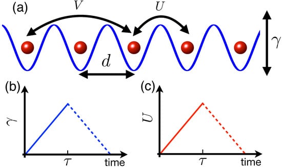
Figure 1. (Color online) The extended Bose-Hubbard Chain and quenching schemes. (a) Nearest-neighbor (U) and next-nearest-neighbor (V) interactions between atoms in a one-dimensional optical lattice (lattice constant d). The tilting of the lattice is denoted by the parameter $\gamma$. We consider a linear quench in (b) $\gamma$ and (c) U towards a non-zero value (solid). When $\gamma$ (U) returns to the initial value (both solid and dashed), this is a hysteresis quench. The rate to quench $\gamma$ (U) is $\alpha$ ($\beta$). See text for details of the soft-core interaction and quenching protocols.

In this work, we investigate chaotic properties of Rydberg-dressed BECs in a one-dimensional (1D) optical lattice in which the dressed interaction leads to a multi-site density–density interaction. In the semiclassical regime, the nonlinear dynamics of the Bose-Hubbard model is captured by a discrete, coupled GP equation. Nonlinear eigenenergies, Bogoliubov spectra as well as Lyapunov exponents of the dressed BEC in the lattice are investigated. We then explore the dynamical stability of the ground state and localized state, where the dependence of the largest and the total number of positive Lyapunov exponents [72,73] on the dressed interaction and system size are explored. We show that at least two positive Lyapunov exponents can be found when the interaction is strong and when the number of sites is equal to or larger than four. This leads to the emergence of hyperchaos in the dynamics. We probe the chaotic dynamics by employing both a linear and a hysteresis quench of the potential bias and dressed interaction [74,75,76].

The paper is organized as follows. In Section 2, the Hamiltonian of the Bose-Hubbard Chain is introduced. The corresponding mean-field approximation and GP equations are given. Methods on calculating the eigenenergy, Bogoliubov spectra, and Lyapunov exponents are briefly introduced. Quench schemes of the potential bias and nonlinear interaction are explained. We explore the static (eigenenergies and Bogoliubov spectra) and dynamical properties (Lyapunov exponents) of the ground state and localized state configurations in Section 3 and Section 4, respectively. Dynamics driven by both the linear and hysteresis quenching parameters are explored with different initial states. In Section 5, we examine the scaling of the Lyapunov exponents with the system size for the two different configurations. We demonstrate, through numerical calculations, that areas of the Poincaré sections are almost linearly proportional to the largest Lyapunov exponent. We conclude our work in Section 6.

2. Model and Method

2.1. Extended Bose-Hubbard Model in the Semiclassical Limit

Our setting consists of a gas of N bosonic atoms at zero temperature confined in a one-dimensional lattice, with the lattice constant d, as depicted in Figure 1a. The Rydberg dressing induces long-range interactions between atoms at different sites. Taking into account the hopping between nearest-neighbor sites, we obtain an extended Bose-Hubbard Hamiltonian of L sites [52] ($\hslash =1$):

$$\begin{array}{ccc}\hfill \hat{H}& =& -J\sum _{⟨i,j⟩}^L{\hat{a}}_i^{†}{\hat{a}}_j+\sum _j^L{\Gamma }_j{\hat{n}}_j+\frac{1}{2}{\hat{H}}_{\mathrm{int}},\hfill \end{array}$$

(1)

where ${\hat{a}}_j\left({\hat{a}}_j^{†}\right)$ is the bosonic annihilation (creation) operator at site j. The tunneling strength J acts only on nearest-neighbor sites, denoted by $⟨·⟩$ in the summation. Here, ${\hat{n}}_j={\hat{a}}_j^{†}{\hat{a}}_j$ is the number operator, while ${\Gamma }_j$ is the local tilting potential. The titling is given by ${\Gamma }_j=-\gamma \left(j-1-\lfloor L/2\rfloor \right)$, where $\lfloor ·\rfloor$ and $\gamma$ are the floor function and level bias between neighboring sites, respectively. The onsite and long-range interactions are described by ${\hat{H}}_{\mathrm{int}}=g{\sum }_j^L{\hat{n}}_j\left({\hat{n}}_j-1\right)+{\sum }_{i,j}^L{\Lambda }_{i,j}{\hat{n}}_i{\hat{n}}_j$. The onsite interaction $g=4\pi a_s/m$ [2] depends on the s-wave scattering length $a_s$ and mass m, where the former can be adjusted by Feshbach resonances [2]. The soft-core shaped long-range interaction is given by ${\Lambda }_{i,j}=C_6{/\left[\right|i-j|}^6{d}^6+R^6]$, with $C_6$ being the dispersion coefficient (Figure 1a). Both the soft-core radius R and $C_6$ can be tuned by laser parameters [48]. In this work, we will restrict our investigation to the onsite, nearest-neighbor (${\Lambda }_{j,j\pm 1}$) and next-nearest-neighbor (${\Lambda }_{j,j\pm 2}$) interactions only, where $R\sim d$. This approximation is valid as the soft-core interaction decays rapidly when the separation between sites is larger than the soft-core radius.

In the semiclassical limit $N\gg 1$, we employ the mean-field approximation where the bosonic operator is described by a classical field ${\psi }_j$, i.e., ${\hat{a}}_j\approx {\psi }_j\sqrt{N}$ and ${\hat{a}}_j^{†}\approx {\psi }_j^{*}\sqrt{N}$, with the normalization condition ${\sum }_j{\left|{\psi }_j\right|}^2=1$. This yields the semiclassical Hamiltonian $\mathcal{H}\approx \hat{H}/N$:

$$\begin{array}{ccc}\hfill \mathcal{H}& =& \sum _j^L{\Gamma }_j|{\psi }_j{|}^2-J\sum _j^L\left({\psi }_{j+1}^{*}{\psi }_j+{\psi }_{j-1}^{*}{\psi }_j\right)+\frac{N}{2}\sum _{i,j}^L{\left|{\psi }_j\right|}^2\left[g\left(|{\psi }_j{|}^2-1\right)+{\Lambda }_{i,j}{\left|{\psi }_i\right|}^2\right].\hfill \end{array}$$

(2)

The dynamics of the classical field ${\psi }_j$ is obtained via the canonical equation $id{\psi }_j/dt=\partial \mathcal{H}/\partial {\psi }_j^{*}$, yielding the coupled GP equations:

$$\begin{array}{ccc}\hfill i{\dot{\psi }}_j& =& -J\left({\psi }_{j+1}+{\psi }_{j-1}\right)+[{\Gamma }_j+W{\left|{\psi }_j\right|}^2+\hfill \\ & & U\left(|{\psi }_{j+1}{|}^2+|{\psi }_{j-1}{|}^2)+V(|{\psi }_{j+2}{|}^2+{\left|{\psi }_{j-2}\right|}^2\right)]{\psi }_j,\hfill \end{array}$$

(3)

where we have defined $W=N({\Lambda }_{j,j}+g)$, $U=N{\Lambda }_{j,j\pm 1}$, and $V=N{\Lambda }_{j,j\pm 2}$ to be the onsite, nearest-neighbor, and next-nearest-neighbor interaction strengths. The onsite interaction W takes into account contributions from both the s-wave and soft-core interactions. We will assume a vanishing onsite interaction, i.e., $W=0$, which allows us to focus on effects induced by the long-range interaction part. To be concrete, we will fix the nearest-neighbor and next-nearest-neighbor interactions at $U=2V$ in the following discussion. Time and energy will be scaled with respect to $1/J$ and J in what follows.

It is convenient to examine the real (${\mathcal{R}}_j=\mathrm{Re}\left[{\psi }_j\right]$) and imaginary components (${\mathcal{I}}_j=\mathrm{Im}\left[{\psi }_j\right]$) of ${\psi }_j$:

$$\begin{array}{ccc}\hfill {\dot{\mathcal{R}}}_j& =& -J\left({\mathcal{I}}_{j+1}+{\mathcal{I}}_{j-1}\right)+[{\Gamma }_j+W{\left|{\psi }_j\right|}^2+\hfill \\ & & U\left(|{\psi }_{j+1}{|}^2+|{\psi }_{j-1}{|}^2)+V(|{\psi }_{j+2}{|}^2+{\left|{\psi }_{j-2}\right|}^2\right)]{\mathcal{I}}_j,\hfill \end{array}$$

(4)

$$\begin{array}{ccc}\hfill {\dot{\mathcal{I}}}_j& =& J\left({\mathcal{R}}_{j+1}+{\mathcal{R}}_{j-1}\right)-[{\Gamma }_j+W{\left|{\psi }_j\right|}^2+\hfill \\ & & U\left(|{\psi }_{j+1}{|}^2+|{\psi }_{j-1}{|}^2)+V(|{\psi }_{j+2}{|}^2+{\left|{\psi }_{j-2}\right|}^2\right)]{\mathcal{R}}_j,\hfill \end{array}$$

(5)

with $|{\psi }_j{|}^2={\mathcal{R}}_j^2+{\mathcal{I}}_j^2$. Both ${\mathcal{R}}_j$ and ${\mathcal{I}}_j$ are real-valued functions of time. We will calculate Lyapunov exponents and the Poincaré sections based on these real functions. Note that ${\mathcal{R}}_j$ and ${\mathcal{I}}_j$ represent mean values of the quadrature of the operator ${\hat{a}}_j$. The quadrature fulfills the commutation relation similar to the position and momentum operator [77]. Hence, the mean values of the quadrature allow us to obtain useful information on the dynamics of the system in phase space. For small systems, $L=2$ or 3, one can also describe the classical field with the canonical phase and particle number decomposition [15,78].

2.2. Nonlinear Eigenenergies and Bogoliubov Spectra

Though the Hamiltonian (2) is Hermitian, the density-dependent nonlinearity prevents us from calculating the eigenenergy through conventional diagonalization. To overcome this, a shooting method will be employed to numerically evaluate the eigenstate ${\overline{\Psi }}_j=[{\overline{\psi }}_1,{\overline{\psi }}_2,\cdots ,{\overline{\psi }}_L]$ and the corresponding eigenenergy ${\epsilon }_j$ self-consistently [71]. A trial solution is seeded into the semiclassical Hamiltonian. It is then diagonalized, leading to a new eigenstate and eigenenergy. This process is iterated until the resulting eigenstate and eigenenergy are obtained self-consistently.

For interacting systems, one can analyze the Bogoliubov spectra ${ϵ}_B$ to understand the stability of the eigenstate. This is achieved by linearizing around a given state $\overline{\Psi }$ (e.g., a fixed point of the semiclassical system), where each component is given by ${\psi }_j={\overline{\psi }}_j+u_j{\mathrm{e}}^{-i{ϵ}_{B}t}-v_j^{*}{\mathrm{e}}^{i{ϵ}_{B}t},$ with $u_j$ and $v_j$ being the probability amplitudes of the Bogoliubov quasiparticles [2]. The dynamics of $u_j$ and $v_j$ are described by the Bogoliubov equations [79,80]:

$$\begin{array}{ccc}\hfill \left(\begin{array}{cc}\mathcal{L}& \mathcal{N}\\ -\mathcal{N}& -\mathcal{L}\end{array}\right)\left(\begin{array}{c}\mathbf{u}\\ \mathbf{v}\end{array}\right)& =& {ϵ}_B\left(\begin{array}{c}\mathbf{u}\\ \mathbf{v}\end{array}\right)\hfill \end{array}$$

(6)

where $\mathcal{L}={\tilde{H}}_0+2U\mathcal{P}-\mu$ and $\mathcal{N}=-U\mathcal{P}$. ${\tilde{H}}_0$ and $\mathcal{P}$ are $L\times L$ block matrices. From Equation (3), we obtain the matrix elements $⟨{\psi }_j|{\tilde{H}}_0|{\psi }_j⟩={\Gamma }_j$, $⟨{\psi }_j\left|{\tilde{H}}_0\right|{\psi }_{j\pm 1}⟩=-J$, $⟨{\psi }_j\left|\mathcal{P}\right|{\psi }_j⟩=|{\overline{\psi }}_{j+1}{|}^2+|{\overline{\psi }}_{j-1}{|}^2+\left(\right|{\overline{\psi }}_{j+2}{|}^2+|{\overline{\psi }}_{j-2}{|}^2)/2$, $⟨{\psi }_j\left|\mathcal{P}\right|{\psi }_{j\pm 1}⟩=2{\overline{\psi }}_{j\pm 1}{\overline{\psi }}_j$ and $⟨{\psi }_j\left|\mathcal{P}\right|{\psi }_{j\pm 2}⟩={\overline{\psi }}_{j\pm 2}{\overline{\psi }}_j$, while other matrix elements are zero. If the Bogoliubov spectra are complex numbers, the state is then dynamically unstable as Bogoliubov quasiparticles grow (decay) exponentially with time, the rate of which is determined by the imaginary part of the spectra.

2.3. Poincaré Sections and Lyapunov Exponents

The emergence of chaos in the dynamics can be characterized by the Poincaré sections and Lyapunov exponents. For L sites, the possible trajectories are the complete set of $\{{\mathcal{R}}_1,\cdots ,{\mathcal{R}}_L,{\mathcal{I}}_1,\cdots ,{\mathcal{I}}_L\}$. Due to the normalization condition, we need to solve a $2L-1$ dimensional system to obtain the dynamics. It is difficult to comprehend the stability of the trajectories in such a high-dimensional phase space. Instead, we project the dynamics to a two-dimensional (2D) Poincaré section to identify the dynamical properties. To calculate the 2D Poincaré section, we record trajectories of selected variables (${\mathcal{R}}_j$, ${\mathcal{I}}_j$) as they cut through the ${\mathcal{U}}_k$ plane ($j\ne k$), provided that ${\dot{\mathcal{U}}}_k>0$. These intersecting points form the 2D Poincaré section. To be specific, we will evaluate the Poincaré section of the variable (${\mathcal{R}}_2$, ${\mathcal{I}}_2$) on the ${\mathcal{U}}_1$ plane.

The strength of the chaos can be measured by the Lyapunov exponents associated with the equations of motion [72,73]. The Lyapunov exponents give the rate of separation between trajectories for a given initial state. As the Lyapunov exponents depend on the initial state, we initially consider both the ground state and a localized state. In a localized state, nearly all the condensate sits in a single site, which can be stable (i.e., the self-trapping state) when the nonlinear interaction is strong. In this work, the Lyapunov exponents ${\lambda }_j$ ($j=1,\cdots ,2L$) are calculated via DynamicalSystems.jl, a fast and reliable Julia library, to determine the dynamics of nonlinear systems [81]. We confirmed with the method in Ref. [72] that it gives consistent data. When there exists at least one positive Lyapunov exponent, the trajectories will separate exponentially, leading to chaotic dynamics. The dynamics is hyperchaotic when there are more than two positive Lyapunov exponents [73].

2.4. Quenching Schemes

In Section 3 and Section 4 we will explore the dynamics of the system with time-dependent parameters via the following quenching schemes:

Scheme$\mathbf{I}$: First, we consider a linear quench of the potential bias [71]. The bias between two neighboring sites is given by the following function:

$$\begin{array}{c}\hfill {\gamma }_L={\gamma }_i+\alpha t,\end{array}$$

(7)

where ${\gamma }_i$ and $\alpha$ are the initial value and quench rate, respectively. With ${\gamma }_i<0$, the quench takes place from $t=0$ to $t=2{\gamma }_f/\alpha$ with ${\gamma }_f=-{\gamma }_i$, depicted by the solid curve in Figure 1b.

Scheme$\mathbf{II}$: Alternatively, we consider a hysteresis quench [74,75,76] where the system begins at ${\gamma }_i$ and then evolves to ${\gamma }_f$. At time $\tau ={\gamma }_f/\alpha$, the potential bias is quenched back towards ${\gamma }_i$. The function describing this scheme is as follows:

$$\begin{array}{c}\hfill {\gamma }_H={\gamma }_f+({\gamma }_i-{\gamma }_f)\frac{|\tau -t|}{\tau }.\end{array}$$

(8)

The corresponding scheme is shown by the solid and dashed curves in Figure 1b.

Scheme$\mathbf{III}$: In addition to quenching the level bias, we also change the two-body interaction strength through a linear ramp:

$$\begin{array}{c}\hfill U_L=U_i+\beta t\end{array}$$

(9)

where $U_i$ is the initial interaction strength and $\beta$ is the quench rate. This is shown by the solid curve in Figure 1c. Note that the next-nearest-neighbor interaction V also depends on time due to the relation $U=2V$.

Scheme$\mathbf{IV}$: The hysteresis counterpart of the interaction quench is given by the following equation:

$$\begin{array}{c}\hfill U_H=U_f+(U_i-U_f)\frac{|{\tau }^{\prime }-t|}{\tau },\end{array}$$

(10)

where $U_f$ is the final interaction strength, with ${\tau }^{\prime }=U_f/\beta$.

3. Stability of the Ground State

3.1. Eigenenergies, Bogoliubov Spectra, and Lyapunov Exponents

Without the nonlinearity, the number of eigenenergies $N_{ϵ}$ is identical to L, the dimension of the semiclassical system. The number of eigenenergies can be larger than L when the interaction is strong. As an example, eigenenergies for $L=3$ as a function of the bias $\gamma$ are shown in Figure 2a. We find that $N_{ϵ}>L$ when $\left|\gamma \right|\lesssim U$, where the nonlinearity dominates. Loops and crossings appear in the eigenenergies, except the highest energy level.

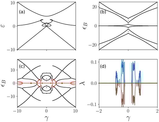
Figure 2. Eigenenergies, Bogoliubov spectra, and Lyapunov exponents when varying the tilt $\gamma$. We show (a) the nonlinear eigenenergy, the Bogoliubov spectra of (b) the ground state and (c) the first excited state, and (d) the Lyapunov exponents of the ground state. The nonlinearity dominates when $\left|\gamma \right|$ is small, leading to loops in the eigenenergy. The Bogoliubov spectra are all real when the system is in the ground state (b). The Bogoliubov spectra have complex components (red region) when the system is in the first-excited state. Positive Lyapunov exponents indicate the system exhibits chaos dynamically, which appear mostly in the loop region of the eigenenergy. Parameters are $L=3$ and $U=2V=5$.

For a given state of the nonlinear system, one obtains $2L$ Bogoliubov spectra, whose values depend on the specific eigenstate and nonlinear interaction strength. The Bogoliubov modes are stable for all $\gamma$ when the system is in the ground state, i.e., the Bogoliubov spectra ${ϵ}_B$ are real, as shown in Figure 2b. This is in contrast to excited eigenstates, whose Bogoliubov spectra have imaginary components. As an example, the Bogoliubov spectra of the first excited state are shown in Figure 2c. The corresponding Bogoliubov mode will decay (grow) exponentially, when the imaginary part is negative (positive).

The chaotic dynamics of the system is characterized by positive Lyapunov exponents. In Figure 2d, Lyapunov exponents are shown for the ground state of the system. When increasing $\gamma$, negative and positive Lyapunov exponents are found in regions where the eigenenergies show loops. The negative and positive Lyapunov exponents appear in pairs with the same absolute values as our system is conservative. In this example, one positive Lyapunov exponent can be found when $\left|\gamma \right|<1$, indicating the presence of chaos. This means that small fluctuations on the ground state could gain exponential growth, and hence drives the system away from the ground state.

To further understand the roles played by the nonlinearity, we calculate eigenenergies as a function of the interaction strength U shown in Figure 3a,b for $L=3$ and $L=5$, respectively. It can be seen that new branches are generated when the nonlinear interaction U is large enough. Lyapunov exponents of the ground state of the nonlinear system are shown in Figure 3c,d. Positive Lyapunov exponents are found in the strongly interacting region, whose values increase with increasing U. Larger Lyapunov exponents mean that the exponential growth of the instability can be even faster. More importantly, the number of Lyapunov exponents now depends on L. For $L=3$, one obtains a single positive Lyapunov exponent when $U\gtrsim 4$. When $L=5$, there are three positive Lyapunov exponents. This indicates that the system enters the so-called hyperchaos regime [82,83,84], where more than one positive Lyapunov exponents can be found in the dynamics. In the two examples, we obtain maximally $L-2$ positive Lyapunov exponents as the energy and particle number are conserved in the Bose-Hubbard Chain.

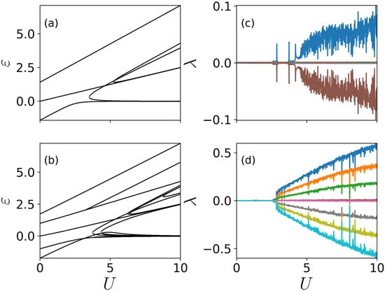
Figure 3. Eigenenergies and Lyapunov exponents as a function of U. We show eigenenergy for (a) $L=3$ and (b) $L=5$ when the trap is balanced ($\gamma =0$). Level crossings are found when the interaction is strong. Starting from the ground state, we calculate Lyapunov exponents for (c) $L=3$ and (d) $L=5$. For a given U, Lyapunov exponents of same value but opposite signs appear in pairs.

3.2. Quench Dynamics

In the linear regime, dynamics of the system will follow the eigenstate adiabatically when slowly quenching the tilt potential. However, the dynamics may deviate from the adiabatic eigenstate in the nonlinear regime, especially when positive Lyapunov exponents are found. This will be illustrated through the quenching of the tilt potential and interaction strength given by Equations (7)–(10). To trigger the instability in the dynamics, we consider a thermal mixed state ${\overline{\Psi }}_j^{\prime }=[{\overline{\psi }}_1{\mathrm{e}}^{i{\theta }_1},{\overline{\psi }}_2{\mathrm{e}}^{i{\theta }_2},\cdots ,{\overline{\psi }}_L{\mathrm{e}}^{i{\theta }_L}]$ around a given state ${\overline{\Psi }}_j$ (the ground state), where ${\theta }_j$ is a random phase distributed uniformly between 0 and $2\pi$[76]. In numerical simulations, we typically consider an ensemble of $M=100$ realizations with a given set of parameters.

We first examine a linear quench of the bias $\gamma$ when the system is prepared in the ground state at ${\gamma }_i=-10$ and $L=3$. The majority of the condensate is located on the first (leftmost) site [$n_1\left(0\right)={\left|{\psi }_1\right|}^2\approx 1$] initially (Figure 4a). In the adiabatic limit and without the nonlinear interaction, the condensate will move to the third well, $n_3\left(\tau \right)\approx 1$, after the quench [71]. The population at this adiabatic limit is shown with a black dot in each panel. The quench dynamics, however, depend on the finite quench rate and the interaction strength. When the interaction is weak, the condensate can be in any of the three sites since the tunneling strength between neighboring sites plays the dominant role. The distribution of the final population is affected by the noise on the initial state and also depends on the final time in the simulations. By increasing U, the population is distributed into a larger region of the phase space, i.e., it occupies larger areas in the $n_3$–$n_1$ plane. By fixing the interaction U, our numerical simulation shows that the smaller $\alpha$ is, the closer the population distribution is to the adiabatic limit.

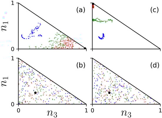
Figure 4. (Color online) Final population distribution of the ground state. The population by quenching $\gamma$ with (a) scheme $\mathbf{I}$ and (b) scheme $\mathbf{II}$ is shown for $L=3$. In the numerical simulation, ${\gamma }_i=-{\gamma }_f=-10$ and the interaction strength is $U=5$. The interaction U is quenched with (c) scheme $\mathbf{III}$ and (d) scheme $\mathbf{IV}$, where $U_i=0$, $U_f=10$ and $\gamma =0$, respectively. In all the figures, the quench rates ($\alpha$ or $\beta$) are 1 (blue), $0.1$ (green), and $0.01$ (red). The total number of trajectories is $M=100$. The target final state is shown as the large black circle.

For the hysteresis quench given by Equation (8), we see that even for $U=5$ (meaning the eigenstate exhibits complicated level crossings) the density mostly returns to their initial state, at least when $\alpha \ll 1$ (Figure 4b). Here, the hysteresis quench has allowed for a large level of reversibility in the dynamics [76] as the chaotic regions have not been triggered. By increasing the quench rate $\alpha$, the population distributions cluster around much smaller regions in the phase space than the one shown in panel (a).

In Figure 4c we quench the interaction according to Equation (9). The initial states depend on the value of $\gamma$. For example, the ground state is $\overline{\Psi }=[0.5,1/\sqrt{2},0.5]$ for $\gamma =0$. The final states are highly dependent on the initial conditions due to the chaos in the dynamics (see the crossing energy levels in Figure 3a and Lyapunov exponent in Figure 3c). We have verified that by increasing $\gamma$, the associated randomness with the final states decreases since the number of crossings in the eigenenergy also decreases.

In case of the hysteresis quench of U, we find that the results (Figure 4d) are similar to the linear quench. When looking at $\gamma =0$, the final states do not return to the initial value. As shown in Figure 3c, the Lyapunov exponent of the ground state becomes positive when $U\gtrsim 4$, which causes the final state to be more random, i.e., to have a broader distribution of the densities. As the tilt $\gamma$ increases, we have verified that chaos is gradually suppressed as the population that localizes in the trap corresponds to the lowest energy state. In order to trigger chaotic dynamics in the tilted case, stronger interactions are generally needed.

4. Stability of the Localized State

4.1. Bogoliubov Spectra and Lyapunov Exponents

In this section, we will explore stability of a situation where the condensate is trapped in a single site. When localized at one end of the lattice, it corresponds to the ground state if the lattice potential is strongly tilted $\left|\gamma \right|\gg 1$. We will examine dynamics of localized states even in the balanced case ($\gamma =0$), partially motivated by the fact that the self-trapped state can be stabilized by strong nonlinear interactions. We will show that dynamical instabilities of localized states will depend strongly on the long-range interaction. To be concrete, we will consider a scenario where the condensate is confined in the second trap from the left of the lattice, i.e., $\overline{\Psi }=[0,1,\cdots ,0]$. In the numerical simulations of the dynamics, uniform density fluctuations are applied to the lattice to trigger the hopping dynamics. This modifies the initial state into $\overline{\Psi }=[\sqrt{\epsilon /L}{e}^{{\varphi }_1},\sqrt{1-\epsilon }{e}^{{\varphi }_2},\cdots ,\sqrt{\epsilon /L}{e}^{{\varphi }_L}]$ with $ϵ\ll 1$ and ${\varphi }_j$ being a random phase. Furthermore, this choice insures that the energy of different initial states are almost identical.

In Figure 5a,b, dynamical unstable regions in the Bogoliubov spectra for $L=3$ and $L=5$ are shown (highlighted with a dark red color). In the unstable region, ${ϵ}_B$ develops imaginary components, which depend on U, $\gamma$ and L. In the case of $L=3$, the condensate is localized in the middle site initially, meaning the Bogoliubov spectra are symmetric with respect to $\gamma$. Figure 5a shows that the system is dynamically unstable when U is small, in particular when the lattice is balanced ($\left|\gamma \right|$ is small). This is not surprising since the localized state is not the ground state, nor does the system support the self-trapped state. By increasing the interaction strength, we note that the localized state returns to a stable configuration when $\left|\gamma \right|$ is small. This means that the localized state becomes a stable, self-trapped state [71]. When $L=5$, the dynamical stability now depends heavily on tilt $\gamma$. When $\gamma >0$, there is a much broader range of unstable regions. This feature is largely due to the fact that the nonsymmetric initial state has higher energies. Therefore, we expect to see qualitatively different dynamics from the various quenching schemes.

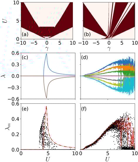
Figure 5. (Color online) Bogoliubov spectra and Lyapunov exponents of the localized state. Dynamically unstable regions (dark red) for (a) $L=3$ and (b) L = 5 are shown as a function of U and $\gamma$. Panels (c,d) give the Lyapunov exponents as a function of U. Random perturbation to the initial state are examined for (e) $L=3$ and (f) $L=5$. The red lines show the maximal Lyapunov exponents in (c,d), correspondingly. Here, $\gamma =0$ in panels (c,d).

The Lyapunov exponents exhibit sensitive dependence on the system size. As shown in Figure 5c, the Lyapunov exponents for $L=3$ show an unusually symmetric shape when $U\gtrsim 4$. The exponents are a smooth function of U and reach maximal value around $U=5$. By further increasing U, the positive Lyapunov exponents decrease. This indicates that the localized configuration could exhibit chaotic dynamics for a large U. For $L=5$ we notice that positive Lyapunov exponents can be found when U is relatively small. A key difference is that there are multiple positive Lyapunov exponents (Figure 5d) where the nonlinear dynamics enters the hyperchaotic regime.

To understand the maximal Lyapunov exponents, we slightly alter the initial state so that we have $\overline{\Psi }=\left[\epsilon ,\sqrt{1-2{\epsilon }^2},\epsilon ,\cdots ,0\right]$, where $\epsilon$ is a small perturbation to the wave function of the traps on either side of the localized site, with $0<\epsilon <0.01$. In Figure 5e,f (corresponding to $L=3$ and 5), the largest Lyapunov exponent ${\lambda }_m$ (red) and Lyapunov exponents obtained with modified initial states (black) are shown (only the positive branch). It shows that a minor change to the initial state will change Lyapunov exponents significantly. However, ${\lambda }_m$ gives an approximate upper bound for all the Lyapunov exponents.

4.2. Quench Dynamics

For $U=5$ and $L=3$, a linear quench (Figure 6a) from ${\gamma }_i=-10$ to ${\gamma }_f=10$ shows strong, self-trapping behavior in the rightmost potential. Ideally, we would expect that by performing a hysteresis quench back towards ${\gamma }_i$, the population would localize in the leftmost site again. However, from Figure 6b, we see that the final state is rather chaotic. Due to the dynamical instability and chaos near $\left|\gamma \right|<1$, the final state deviates from the initial state. In panels (c) and (d), we quench according to Equations (9) and (10), respectively. The dynamics shows that in both cases, the localized initial state loses population to the outer potential wells in an approximately equal manner for both the linear and hysteresis quenches. The strong, nonlinear interactions in the initial localized trap repel the condensate symmetrically between the two neighboring traps. Additionally, we notice that in panel (d), the population could be $n_1=n_3\approx 0$, meaning that the final state is exactly equal to the initial state. We have achieved full reversibility with the hysteresis dynamics in these simulations. As shown in panel (c), this is not the case where the populations are always $n_1\approx n_2>0$, implying that the strong, two-body interactions prevent the complete localization of the condensate in a single site.

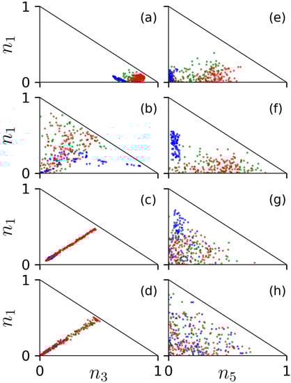
Figure 6. (Color online) Final population distribution of the localized state. The first and second row show the linear and hysteresis quench of $\gamma$. Here, $U=5$, ${\gamma }_i=-{\gamma }_f=10$. The third and fourth row show the linear and hysteresis quench of U, with $U_i=0$, $U_f=10$, and $\gamma =0$. In (a–d), we consider three sites and the initial thermal state is $\overline{\Psi }=[0.1e^{i{\varphi }_1},\sqrt{0.98}{e}^{i{\varphi }_2},0.1e^{{\varphi }_3}]$, with ${\varphi }_j$ ($j=1,2,3$) being a random number in $[0,2\pi ]$. In (e–h), $L=5$ and the initial state is $\overline{\Psi }=[\sqrt{0.005}{e}^{i{\varphi }_1},\sqrt{0.98}{e}^{i{\varphi }_2},\sqrt{0.005}{e}^{i{\varphi }_3},\sqrt{0.005}{e}^{i{\varphi }_4},{\sqrt{0.005}}^{i{\varphi }_5}]$, with ${\varphi }_j$ ($j=1,\cdots ,5$) being randomly distributed in $[0,2\pi ]$. The small fraction in sites other than the localized state is used to trigger the hopping dynamics. The other parameters are the same as the ones in Figure 4.

We now move on to examine the dynamics for the five-site system. Without two-body interactions, linearly quenching from ${\gamma }_i$ to ${\gamma }_f$ will force the atoms towards the rightmost trap. However, from Figure 6e, we see that the occupation is never very much greater than $n_5\approx 0.5$, even for the slowest quenching rates considered in the simulation. When the quench rate is fast ($\alpha \sim 1$), we find less occupation in both the first and last sites, implying that the occupation has been spread amongst the remaining sites. In panel (f), the hysteresis counterpart is shown. Now the population should tend towards $n_1\approx 1$. However, this is not what is found in the numerical simulations. The populations distribute randomly in all sites. In panels (g) and (h), the dynamics is qualitatively different from the $L=3$ scenario. The symmetry between the densities of the two outermost sites is completely lost and is replaced with a chaotic distribution, largely due to the presence of hyperchaos (see Figure 5d).

5. Discussion

In the following, we will discuss how the maximal and total number of Lyapunov exponents depend on the system size and initial state, focusing on parameter regimes where the nonlinear interaction cannot be neglected, i.e., chaos and hyperchaos are expected in the dynamics. In general, Lyapunov exponents depend on the input state of the calculation [72]. Two different initial states, i.e., the ground state and the localized state, will be examined in detail.

In Figure 7a the largest Lyapunov exponent ${\lambda }_m$ for the ground state configuration is shown. When $2\le L\le 4$, the values of ${\lambda }_m$ are generally small. This is due to the fact that chaos has not been triggered (see Figure 5b,c). When $L>4$, the situation changes as chaos is already found with the given U. We find that ${\lambda }_m$ decreases gradually when $U=3$ and $U=5$ for larger L. On the other hand, the total number of positive Lyapunov exponents $\eta$ is seen to increase almost linearly with L when $U=3$ and $U=5$, depicted in Figure 7b. More importantly, $\eta >2$ when $L>4$ for both $U=3$ and $U=5$, i.e., the dynamics is hyperchaotic. On the other hand, $\eta$ decreases and deviates from the linear dependence on L when L is large, e.g., at $L=10$ when $U=3$ and $L=14$ when $U=5$. In general, the linear relation holds up to a larger L for larger U. It has recently been shown that the largest Lyapunov exponents in the BH model can be obtained from the echo dynamics of the condensate [85]. A similar technique could be applied to extract the largest Lyapunov exponents studied here.

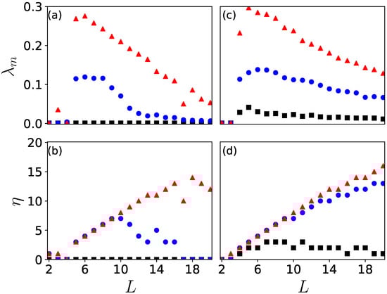
Figure 7. (Color online) Lyapunov Exponents vs. System Size. The maximum Lyapunov exponent and total number of positive Lyapunov exponents are shown in (a,b) for the ground state configuration. Panels (c,d) show the same quantity for the localized state. The larger the value of U is, the larger the maximal Lyapunov exponent. The maximal Lyapunov exponent decreases with increasing L. The number of Lyapunov exponents increases and then decreases with increasing L. For the localized state, $\eta$ increases almost linearly with increasing L. In each panel, $U=1$ (square), 3 (circle), and 5 (triangle).

Figure 7c,d show both ${\lambda }_m$ and $\eta$ for the the localized state. In this case, ${\lambda }_m$ is largest when $L=5$ and decreases with increasing L for $U=3$ and $U=5$. Compared to the ground state, a visible difference is that ${\lambda }_m\ne 0$ when $U=1$ for the localized state. Their values, however, are smaller than the one for $U=3$ and $U=5$. This implies that it will be difficult to observe chaotic dynamics with this level of nonlinear interactions. On the other hand, $\eta$ increases with increasing U. When $L>10$, $\eta$ still increases with L, slightly deviating from the linear scaling with L. A similar dependence is also found for stronger nonlinear interactions, as demonstrated with $U=5$ in panel (d). For such states, $\eta >1$ can be seen even with a relatively weak interaction (e.g., $U=1$), leading to more pronounced hyperchaotic dynamics.

The total number of nonlinear differential equations is $2L$ (the real and imaginary parts of ${\psi }_j$). For conservative systems, the number of positive and negative Lyapunov exponents are the same, and the sum of the Lyapunov exponents is zero. These features can be seen, e.g., in Figure 2d. Our numerical simulations show that the maximal number of positive Lyapunov exponents is $L-2$ (see Figure 7b when $U=5$ and $L\le 11$ and Figure 7d when $U=5$ and $L\le 14$). As the extended Bose-Hubbard model is a Hamiltonian system, not only does the sum of the Lyapunov exponents vanish, but conservative quantities such as the energy and particle number are also found in the dynamics. This indicates that the maximal number of the Lyapunov exponents is $L-2$ and not L. For a sufficiently large L, the total number of positive Lyapunov exponents is smaller than $L-2$ as the nonlinear interaction becomes smaller. For the ground state, one can estimate the interaction energy for a given site to be approximately $2(U+V)/L^2$, i.e., the mean local interaction energy decreases with increasing L.

The chaotic dynamics depends strongly on the largest Lyapunov exponents ${\lambda }_m$, which is considered to be an indication of chaos in the dynamics. To illustrate this, the Poincaré section on the ${\mathcal{U}}_1$ plane for different system sizes is shown in Figure 8, showing that profiles of the Poincaré section depend on the system size and the initial state. The area is largest when $L=5$ (Figure 8a) and decreases with increasing L in the case of the ground state (Figure 8b,c). For different L, the profile of the Poincaré section is largely symmetric with respect to ${\mathcal{R}}_2=0$ and ${\mathcal{I}}_2=0$. In the case of the localized state, similar dependence on L is found, as depicted in Figure 8d–f. We note two differences when compared to the ground state. First, the profile of the Poincaré section displays symmetry with respect to ${\mathcal{I}}_2=0$ but not ${\mathcal{R}}_2=0$. Second, the areas of the Poincaré section in the localized state are slightly larger as the corresponding ${\lambda }_m$ is larger (see Figure 7a,c).

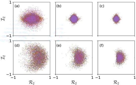
Figure 8. (Color online) Poincaré Sections of the ground state and localized state on the ${\mathcal{U}}_1$-plane. The Poincaré sections are shown for the ground state (a–c) and the localized state (d–f). Each point represents a numerical realization. We consider $L=5$ (a,d), $L=10$ (b,e), and $L=20$ (c,f). Other parameters are $U=3$ and $\gamma =0$.

The area is largely determined by the largest Lyapunov exponent. To verify this, we find the area of the Poincaré section approximately by numerically fitting the Poincaré section, as shown in Figure 9. For the ground state, the dependence of the fitted area and ${\lambda }_m$ on L agrees well when $U=5$. For $U=3$, a good agreement is also found when $L\ge 8$. When $L=5$ and $L=7$, the fitted areas differ largely from the corresponding ${\lambda }_m$. This discrepancy might be caused by the fact that the relatively weak nonlinear interaction leads to uncertainties in calculating the Lyapunov exponent. For the localized state, the agreement is improved in general for both $U=3$ and $U=5$. This suggests that the discrepancy in the ground state could be a boundary effect when L is small, as the localized state suffers less from the boundary effect.

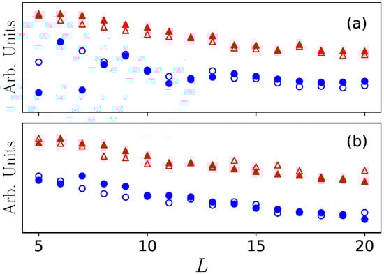
Figure 9. (Color online) Areas of the Poincaré Sections. We compare the fitted area (open shapes) of the Poincaré section with ${\lambda }_m$ (solid) for both the ground state (a) and the localized state (b), respectively. The blue circles are for $U=3$, and red triangles for $U=5$. In both situations, $\gamma =0$.

6. Conclusions and Outlook

We investigated the chaotic and hyperchaotic dynamics of a one-dimensional Bose-Hubbard Chain of Rydberg-dressed BECs in the semiclassical regime. We showed that both the ground state and localized state could have positive Lyapunov exponents even though the corresponding Bogoliubov spectra were real-valued. As a result, small perturbations to these states led to large fluctuations, which were captured by the quench dynamics. The vastly different population distribution after the quench provided evidence of chaos where the former could be measured experimentally. We found that hyperchaos emerges in both the ground and localized states when the nonlinear interaction is strong and L is large. The total number of positive Lyapunov exponents, $\eta$, is bound by $L-2$ ($L\ge 3$). We showed that $\eta$ grows with the system size L when U is large. So far, our investigations have been focused on the semiclassical regime. There has been exploration into the relationships between chaos and quantum entanglement [86]. Moreover, quantum chaos can be seen by analyzing the statistics of the eigenspectra on the Bose-Hubbard model with onsite [87] and long-range interactions [88,89]. It is therefore worthwhile to explore chaos and hyperchaos as well as the thermalization of the Rydberg atoms in the quantum regime.

References

- Robert, P.S.; Zoran, H. Effects of Interactions on Bose-Einstein Condensation of an Atomic Gas. In Physics of Quantum Fluids: New Trends and Hot Topics in Atomic and Polariton Condensates; Alberto, B., Michele, M., Eds.; Springer: Berlin/Heidelberg, Germany, 2013; pp. 341–359. [Google Scholar]
- Pethick, C.J.; Smith, H. Microscopic theory of the Bose gas. In Bose–Einstein Condensation in Dilute Gases; Cambridge University Press: Cambridge, UK, 2008. [Google Scholar]
- Leonardo, F.; Chiara, F.; Jessica, E.L.; Massimo, I. Bose-Einstein condensate in an optical lattice with tunable spacing: Transport and static properties. Opt. Express 2005, 13, 4303–4313. [Google Scholar]
- Smerzi, A.; Fantoni, S.; Giovanazzi, S.; Shenoy, S.R. Quantum coherent atomic tunneling between two trapped bose-einstein condensates. Phys. Rev. Lett. 1997, 79, 4950–4953. [Google Scholar] [CrossRef]
- Manjun, M.R.; Navarro, R.; Carretero-González, R. Solitons riding on solitons and the quantum newton’s cradle. Phys. Rev. E 2016, 93, 022202. [Google Scholar]
- Anderson, B.P.; Haljan, P.C.; Regal, C.A.; Feder, D.L.; Collins, L.A.; Clark, C.W.; Cornell, E.A. Watching dark solitons decay into vortex rings in a bose-einstein condensate. Phys. Rev. Lett. 2001, 86, 2926–2929. [Google Scholar] [CrossRef] [PubMed]
- Zachary, D.; Michael, B.; Christopher, S.; Lene Vestergaard, H. Observation of quantum shock waves created with ultra- compressed slow light pulses in a bose-einstein condensate. Science 2001, 293, 663–668. [Google Scholar]
- Denschlag, J.; Simsarian, J.E.; Feder, D.L.; Clark, C.W.; Collins, L.A.; Cubizolles, J.; Deng, L.; Hagley, E.W.; Helmerson, K.; Phillips, W.D.; et al. Generating solitons by phase engineering of a bose-einstein condensate. Science 2000, 287, 97–101. [Google Scholar] [CrossRef] [PubMed]
- Burger, S.; Bongs, K.; Dettmer, S.; Ertmer, W.; Sengstock, K.; Sanpera, A.; Shlyapnikov, G.V.; Lewenstein, M. Dark solitons in bose-einstein condensates. Phys. Rev. Lett. 1999, 83, 5198–5201. [Google Scholar] [CrossRef]
- Cornish, S.L.; Thompson, S.T.; Wieman, C.E. Formation of bright matter-wave solitons during the collapse of attractive bose-einstein condensates. Phys. Rev. Lett. 2006, 96, 170401. [Google Scholar] [CrossRef]
- Khaykovich, L.; Schreck, F.; Ferrari, G.; Bourdel, T.; Cubizolles, J.; Carr, L.D.; Castin, Y.; Salomon, C. Formation of a matter-wave bright soliton. Science 2002, 296, 1290–1293. [Google Scholar] [CrossRef]
- Strecker, K.E.; Partridge, G.B.; Truscott, A.G.; Hulet, R.G. Formation and propagation of matter-wave soliton trains. Nature 2002, 417, 150–153. [Google Scholar] [CrossRef]
- Kinoshita, T.; Wenger, T.; Weiss, D.S. A quantum newton’s cradle. Nature 2006, 440, 900–903. [Google Scholar] [CrossRef]
- Xia, B.; Hai, W.; Chong, G. Stability and chaotic behavior of a two-component Bose-Einstein condensate. Phys. Lett. Sect. A Gen. At. Solid State Phys. 2006, 351, 136–142. [Google Scholar] [CrossRef]
- Liu, B.; Fu, L.B.; Yang, S.P.; Liu, J. Josephson oscillation and transition to self-trapping for Bose-Einstein condensates in a triple-well trap. Phys. Rev. A 2007, 75, 033601. [Google Scholar] [CrossRef]
- Graefe, E.M.; Korsch, H.J.; Witthaut, D. Mean-field dynamics of a Bose-Einstein condensate in a time-dependent triple-well trap: Nonlinear eigenstates, Landau-Zener models, and stimulated Raman adiabatic passage. Phys. Rev. A 2006, 73, 013617. [Google Scholar] [CrossRef]
- Viscondi, T.F.; Furuya, K. Dynamics of a Bose-Einstein condensate in a symmetric triple-well trap. J. Phys. A Math. Theor. 2011, 44, 175301. [Google Scholar] [CrossRef]
- Li, L.; Wang, B.; Lü, X.Y.; Wu, Y. Chaos-related Localization in Modulated Lattice Array. Annalen der Physik 2018, 530, 1700218. [Google Scholar] [CrossRef]
- Chong, G.; Hai, W.; Xie, Q. Controlling chaos in a weakly coupled array of Bose-Einstein condensates. Phys. Rev. E 2005, 71, 016202. [Google Scholar] [CrossRef]
- Liu, J.; Fu, L.; Ou, B.Y.; Chen, S.G.; Choi, D.I.; Wu, B.; Niu, Q. Theory of nonlinear Landau-Zener tunneling. Phys. Rev. A 2002, 66, 023404. [Google Scholar] [CrossRef]
- Liu, J.; Wu, B.; Niu, Q. Nonlinear Evolution of Quantum States in the Adiabatic Regime. Phys. Rev. Lett. 2003, 90, 170404. [Google Scholar] [CrossRef]
- Albiez, M.; Gati, R.; Fölling, J.; Hunsmann, S.; Cristiani, M.; Oberthaler, M.K. Direct observation of tunneling and nonlinear self-trapping in a single bosonic josephson junction. Phys. Rev. Lett. 2005, 95, 010402. [Google Scholar] [CrossRef]
- Zibold, T.; Nicklas, E.; Gross, C.; Oberthaler, M.K. Classical bifurcation at the transition from rabi to Josephson dynamics. Phys. Rev. Lett. 2010, 105, 204101. [Google Scholar] [CrossRef]
- Gotlibovych, I.; Schmidutz, T.F.; Gaunt, A.L.; Navon, N.; Smith, R.P.; Hadzibabic, Z. Observing properties of an interacting homogeneous bose-einstein condensate: Heisenberg-limited momentum spread, interaction energy, and free-expansion dynamics. Phys. Rev. A 2014, 89, 061604. [Google Scholar] [CrossRef]
- Gaunt, A.L.; Schmidutz, T.F.; Gotlibovych, I.; Smith, R.P.; Hadzibabic, Z. Bose-einstein condensation of atoms in a uniform potential. Phys. Rev. Lett. 2013, 110, 200406. [Google Scholar] [CrossRef] [PubMed]
- Schmidutz, T.F.; Gotlibovych, I.; Gaunt, A.L.; Smith, R.P.; Navon, N.; Hadzibabic, Z. Quantum joule-thomson effect in a saturated homogeneous bose gas. Phys. Rev. Lett. 2014, 112, 040403. [Google Scholar] [CrossRef]
- Buonsante, P.; Penna, V. Some remarks on the coherent-state variational approach to nonlinear boson models. J. Phys. A Math. Theor. 2008, 41, 175301. [Google Scholar] [CrossRef]
- Hai, W.; Rong, S.; Zhu, Q. Discrete chaotic states of a Bose-Einstein condensate. Phys. Rev. E 2008, 78, 066214. [Google Scholar] [CrossRef] [PubMed]
- Sinha, S.; Sinha, S. Chaos and Quantum Scars in Bose-Josephson Junction Coupled to a Bosonic Mode. Phys. Rev. Lett. 2020, 125, 134101. [Google Scholar] [CrossRef] [PubMed]
- Boukobza, E.; Moore, M.G.; Cohen, D.; Vardi, A. Nonlinear phase dynamics in a driven bosonic josephson junction. Phys. Rev. Lett. 2010, 104, 240402. [Google Scholar] [CrossRef]
- Pedri, P.; Santos, L. Two-Dimensional Bright Solitons in Dipolar Bose-Einstein Condensates. Phys. Rev. Lett. 2005, 95, 200404. [Google Scholar] [CrossRef] [PubMed]
- Tikhonenkov, I.; Malomed, B.A.; Vardi, A. Anisotropic Solitons in Dipolar Bose-Einstein Condensates. Phys. Rev. Lett. 2008, 100, 090406. [Google Scholar] [CrossRef] [PubMed]
- Nath, R.; Pedri, P.; Santos, L. Phonon Instability with Respect to Soliton Formation in Two-Dimensional Dipolar Bose-Einstein Condensates. Phys. Rev. Lett. 2009, 102, 050401. [Google Scholar] [CrossRef]
- Cuevas, J.; Malomed, B.A.; Kevrekidis, P.G.; Frantzeskakis, D.J. Solitons in quasi-one-dimensional Bose-Einstein condensates with competing dipolar and local interactions. Phys. Rev. A 2009, 79, 053608. [Google Scholar] [CrossRef]
- Young-S, L.E.; Muruganandam, P.; Adhikari, S.K. Dynamics of quasi-one-dimensional bright and vortex solitons of a dipolar Bose–Einstein condensate with repulsive atomic interaction. J. Phys. B At. Mol. Opt. Phys. 2011, 44, 101001. [Google Scholar] [CrossRef]
- Lahaye, T.; Pfau, T.; Santos, L. Mesoscopic ensembles of polar bosons in triple-well potentials. Phys. Rev. Lett. 2010, 104, 170404. [Google Scholar] [CrossRef]
- Xiong, B.; Fischer, U.R. Interaction-induced coherence among polar bosons stored in triple-well potentials. Phys. Rev. A 2013, 88, 063608. [Google Scholar] [CrossRef]
- Gallemí, A.; Guilleumas, M.; Mayol, R.; Sanpera, A. Role of anisotropy in dipolar bosons in triple-well potentials. Phys. Rev. A 2013, 88, 063645. [Google Scholar] [CrossRef]
- Köberle, P.; Cartarius, H.; Fabčič, T.; Main, J.; Wunner, G. Bifurcations, order and chaos in the bose–einstein condensation of dipolar gases. New J. Phys. 2009, 11, 023017. [Google Scholar] [CrossRef]
- Andreev, P.A. Quantum hydrodynamic theory of quantum fluctuations in dipolar bose–einstein condensate. Chaos An Interdiscip. J. Nonlinear Sci. 2021, 31, 023120. [Google Scholar] [CrossRef]
- Xiong, B.; Gong, J.; Pu, H.; Bao, W.; Li, B. Symmetry breaking and self-trapping of a dipolar Bose-Einstein condensate in a double-well potential. Phys. Rev. A 2009, 79, 013626. [Google Scholar] [CrossRef]
- Abad, M.; Guilleumas, M.; Mayol, R.; Pi, M.; Jezek, D.M. A dipolar self-induced bosonic Josephson junction. Europhys. Lett. 2011, 94, 10004. [Google Scholar] [CrossRef]
- Wang, C.; Kevrekidis, P.G.; Frantzeskakis, D.J.; Malomed, B.A. Effects of long-range nonlinear interactions in double-well potentials. Phys. D Nonlinear Phenom. 2011, 240, 805–813. [Google Scholar] [CrossRef]
- Adhikari, S.K. Self-trapping of a dipolar Bose-Einstein condensate in a double well. Phys. Rev. A 2014, 89, 043609. [Google Scholar] [CrossRef]
- Zhang, A.-X.; Xue, J.-K. Dipolar-induced interplay between inter-level physics and macroscopic phase transitions in triple-well potentials. J. Phys. B At. Mol. Opt. Phys. 2012, 45, 145305. [Google Scholar] [CrossRef]
- Fortanier, R.; Zajec, D.; Main, J.; Wunner, G. Dipolar Bose–Einstein condensates in triple-well potentials. J. Phys. B At. Mol. Opt. Phys. 2013, 46, 235301. [Google Scholar] [CrossRef][Green Version]
- Bouchoule, I.; Molmer, K. Spin squeezing of atoms by the dipole interaction in virtually excited Rydberg states. Phys. Rev. A 2002, 65, 041803. [Google Scholar] [CrossRef]
- Henkel, N.; Nath, R.; Pohl, T. Three-dimensional roton excitations and supersolid formation in rydberg-excited bose-einstein condensates. Phys. Rev. Lett. 2010, 104, 195302. [Google Scholar] [CrossRef] [PubMed]
- Honer, J.; Weimer, H.; Pfau, T.; Büchler, H.P. Collective many-body interaction in rydberg dressed atoms. Phys. Rev. Lett. 2010, 105, 160404. [Google Scholar] [CrossRef]
- Pupillo, G.; Micheli, A.; Boninsegni, M.; Lesanovsky, I.; Zoller, P. Strongly correlated gases of rydberg-dressed atoms: Quantum and classical dynamics. Phys. Rev. Lett. 2010, 104, 223002. [Google Scholar] [CrossRef] [PubMed]
- Johnson, J.E.; Rolston, S.L. Interactions between Rydberg-dressed atoms. Phys. Rev. A 2010, 82, 033412. [Google Scholar] [CrossRef]
- Li, W.; Hamadeh, L.; Lesanovsky, I. Probing the interaction between Rydberg-dressed atoms through interference. Phys. Rev. A 2012, 85, 053615. [Google Scholar] [CrossRef]
- DeSalvo, B.J.; Aman, J.A.; Gaul, C.; Pohl, T.; Yoshida, S.; Burgdörfer, J.; Hazzard, K.R.A.; Dunning, F.B.; Killian, T.C. Rydberg-blockade effects in autler-townes spectra of ultracold strontium. Phys. Rev. A 2016, 93, 022709. [Google Scholar] [CrossRef]
- Hsueh, C.-H.; Wang, C.-W.; Wu, W.-C. Vortex structures in a rotating rydberg-dressed bose-einstein condensate with the lee-huang-yang correction. Phys. Rev. A 2020, 102, 063307. [Google Scholar] [CrossRef]
- Maucher, F.; Henkel, N.; Saffman, M.; Królikowski, W.; Skupin, S.; Pohl, T. Rydberg-induced solitons: Three-dimensional self-trapping of matter waves. Phys. Rev. Lett. 2011, 106, 170401. [Google Scholar] [CrossRef] [PubMed]
- Cinti, F.; MacRì, T.; Lechner, W.; Pupillo, G.; Pohl, T. Defect-induced supersolidity with soft-core bosons. Nat. Commun. 2014, 5, 4235. [Google Scholar] [CrossRef] [PubMed]
- Hsueh, C.H.; Tsai, Y.C.; Wu, W.C. Excitations of one-dimensional supersolids with optical lattices. Phys. Rev. A 2016, 93, 063605. [Google Scholar] [CrossRef]
- McCormack, G.; Nath, R.; Li, W. Dynamical excitation of maxon and roton modes in a Rydberg-Dressed Bose-Einstein Condensate. Phys. Rev. A 2020, 102, 023319. [Google Scholar] [CrossRef]
- Lauer, A.; Muth, D.; Fleischhauer, M. Transport-induced melting of crystals of Rydberg dressed atoms in a one-dimensional lattice. New J. Phys. 2012, 14, 095009. [Google Scholar] [CrossRef][Green Version]
- Lan, Z.; Minar, J.; Levi, E.; Li, W.; Lesanovsky, I. Emergent Devil’s Staircase without Particle-Hole Symmetry in Rydberg Quantum Gases with Competing Attractive and Repulsive Interactions. Phys. Rev. Lett. 2015, 115, 203001. [Google Scholar] [CrossRef]
- Angelone, A.; Mezzacapo, F.; Pupillo, G. Superglass Phase of Interaction-Blockaded Gases on a Triangular Lattice. Phys. Rev. Lett. 2016, 116, 135303. [Google Scholar] [CrossRef]
- Chougale, Y.; Nath, R. Ab initio calculation of Hubbard parameters for Rydberg-dressed atoms in a one-dimensional optical lattice. J. Phys. B At. Mol. Opt. Phys. 2016, 49, 144005. [Google Scholar] [CrossRef]
- Li, Y.; Geißler, A.; Hofstetter, W.; Li, W. Supersolidity of lattice bosons immersed in strongly correlated Rydberg dressed atoms. Phys. Rev. A 2018, 97, 023619. [Google Scholar] [CrossRef]
- Zhou, Y.; Li, Y.; Nath, R.; Li, W. Quench dynamics of Rydberg-dressed bosons on two-dimensional square lattices. Phys. Rev. A 2020, 101, 013427. [Google Scholar] [CrossRef]
- Barbier, M.; Geißler, A.; Hofstetter, W. Decay-dephasing-induced steady states in bosonic rydberg-excited quantum gases in an optical lattice. Phys. Rev. A 2019, 99, 033602. [Google Scholar] [CrossRef]
- Jau, Y.Y.; Hankin, A.M.; Keating, T.; Deutsch, I.H.; Biedermann, G.W. Entangling atomic spins with a Rydberg-dressed spin-flip blockade. Nat. Phys. 2016, 12, 3487. [Google Scholar] [CrossRef]
- Zeiher, J.; van Bijnen, R.; Schauß, P.; Hild, S.; Choi, J.Y.; Pohl, T.; Bloch, I.; Gross, C. Many-body interferometry of a Rydberg-dressed spin lattice. Nat. Phys. 2016, 12, 3835. [Google Scholar] [CrossRef]
- Zeiher, J.; Choi, J.Y.; Rubio-Abadal, A.; Pohl, T.; Van Bijnen, R.; Bloch, I.; Gross, C. Coherent many-body spin dynamics in a long-range interacting Ising chain. Phys. Rev. X 2017, 7, 041063. [Google Scholar] [CrossRef]
- Guardado-Sanchez, E.; Spar, B.M.; Schauss, P.; Belyansky, R.; Young, J.T.; Bienias, P.; Gorshkov, A.V.; Iadecola, T.; Bakr, W.S. Quench Dynamics of a Fermi Gas with Strong Long-Range Interactions. arXiv 2020, arXiv:2010.05871. [Google Scholar]
- Borish, V.; Marković, O.; Hines, J.A.; Rajagopal, S.V.; Schleier-Smith, M. Transverse-Field Ising Dynamics in a Rydberg-Dressed Atomic Gas. Phys. Rev. Lett. 2020, 124, 063601. [Google Scholar] [CrossRef]
- McCormack, G.; Nath, R.; Li, W. Nonlinear dynamics of Rydberg-dressed Bose-Einstein condensates in a triple-well potential. Phys. Rev. A 2020, 102, 063329. [Google Scholar] [CrossRef]
- Wolf, A.; Swift, J.B.; Swinney, H.L.; Vastano, J.A. Determining Lyapunov exponents from a time series. Phys. D Nonlinear Phenom. 1985, 16, 285–317. [Google Scholar] [CrossRef]
- Andreev, A.V.; Balanov, A.G.; Fromhold, T.M.; Greenaway, M.T.; Hramov, A.E.; Li, W.; Makarov, V.V.; Zagoskin, A.M. Emergence and control of complex behaviors in driven systems of interacting qubits with dissipation. NPJ Quantum Inf. 2021, 7, 1–7. [Google Scholar] [CrossRef]
- Eckel, S.; Lee, J.G.; Jendrzejewski, F.; Murray, N.; Clark, C.W.; Lobb, C.J.; Phillips, W.D.; Edwards, M.; Campbell, G.K. Hysteresis in a quantized superfluid ’atomtronic’ circuit. Nature 2014, 506, 200–203. [Google Scholar] [CrossRef] [PubMed]
- Trenkwalder, A.; Spagnolli, G.; Semeghini, G.; Coop, S.; Landini, M.; Castilho, P.; Pezzè, L.; Modugno, G.; Inguscio, M.; Smerzi, A.; et al. Quantum phase transitions with parity-symmetry breaking and hysteresis. Nat. Phys. 2016, 12, 826–829. [Google Scholar] [CrossRef]
- Bürkle, R.; Vardi, A.; Cohen, D.; Anglin, J.R. Probabilistic hysteresis in integrable and chaotic isolated hamiltonian systems. Phys. Rev. Lett. 2019, 123, 114101. [Google Scholar] [CrossRef]
- Scully, M.O.; Zubairy, M.S. Quantum Optics, 1st ed.; Cambridge University Press: Cambridge, UK, 1997. [Google Scholar]
- Castro, E.R.; Chávez-Carlos, J.; Roditi, I.; Santos, L.F.; Hirsch, J.G. Quantum-classical correspondence of a system of interacting bosons in a triple-well potential. arXiv 2021, arXiv:2105.10515. [Google Scholar] [CrossRef]
- Dey, A.; Cohen, D.; Vardi, A. Adiabatic Passage through Chaos. Phys. Rev. Lett. 2018, 121, 250405. [Google Scholar] [CrossRef] [PubMed]
- Dey, A.; Cohen, D.; Vardi, A. Many-body adiabatic passage: Quantum detours around chaos. Phys. Rev. A 2019, 99, 033623. [Google Scholar] [CrossRef]
- Datseris, G. Dynamicalsystems.jl: A julia software library for chaos and nonlinear dynamics. J. Open Source Softw. 2018, 3, 598. [Google Scholar] [CrossRef]
- Baier, G.; Klein, M. Maximum hyperchaos in generalized Hénon maps. Phys. Lett. A 1990, 151, 281–284. [Google Scholar] [CrossRef]
- Baier, G.; Sahle, S. Design of hyperchaotic flows. Phys. Rev. E 1995, 51, R2712–R2714. [Google Scholar] [CrossRef]
- Kapitaniak, T.; Thylwe, K.-E.; Cohen, I.; Wojewoda, J. Chaos-hyperchaos transition. Chaos Solitons Fractals 1995, 5, 2003–2011. [Google Scholar] [CrossRef]
- Tarkhov, A.E.; Wimberger, S.; Fine, B.V. Extracting lyapunov exponents from the echo dynamics of bose-einstein condensates on a lattice. Phys. Rev. A 2017, 96, 023624. [Google Scholar] [CrossRef]
- Lerose, A.; Pappalardi, S. Bridging entanglement dynamics and chaos in semiclassical systems. Phys. Rev. A 2020, 102, 032404. [Google Scholar] [CrossRef]
- Pausch, L.; Carnio, E.G.; Rodríguez, A.; Buchleitner, A. Chaos and Ergodicity across the Energy Spectrum of Interacting Bosons. Phys. Rev. Lett. 2021, 126, 150601. [Google Scholar] [CrossRef]
- Kollath, C.; Roux, G.; Biroli, G.; Läuchli, A.M. Statistical properties of the spectrum of the extended Bose-Hubbard model. J. Stat. Mech. 2010, 2010, P08011. [Google Scholar] [CrossRef]
- Chen, Y.; Cai, Z. Persistent oscillations versus thermalization in the quench dynamics of quantum gases with long-range interactions. Phys. Rev. A 2020, 101, 023611. [Google Scholar] [CrossRef]
Publisher’s Note: MDPI stays neutral with regard to jurisdictional claims in published maps and institutional affiliations. |
© 2021 by the authors. Licensee MDPI, Basel, Switzerland. This article is an open access article distributed under the terms and conditions of the Creative Commons Attribution (CC BY) license (https://creativecommons.org/licenses/by/4.0/).