A PSO-SVM for Burst Header Packet Flooding Attacks Detection in Optical Burst Switching Networks

Abstract

An Optical Burst Switching (OBS) network is vulnerable to Burst Header Packet (BHP) flooding attack. In flooding attacks, edge nodes send BHPs at a high rate to reserve bandwidth for unrealized data bursts, which leads to a waste of bandwidth, a decrease in network performance, and massive data loss. Machine learning techniques are utilized to detect this attack in the OBS network. In this paper, we propose a particle swarm optimization–support vector machine (PSO-SVM) model for detecting BHP flooding attacks, in which the PSO is used to optimize the parameters of the SVM. We use the dataset provided by the UCI warehouse to train and test the model. The experimental results show that the detection accuracy of the PSO-SVM model reaches 95.0%, which is 9.4%, 9.6%, 20.7%, 8% higher than naïve Bayes, SVM, k-nearest neighbor, and decision tree. Although DCNN outperforms our model, it requires more processing and training time. Collectively, our approach is effective and high-efficiency in detecting flooding attacks in optical burst switching networks and maintaining network stability and security.

1. Introduction

In an optical network, there are three main optical switching technologies, namely, Optical Circuit Switching (OCS), Optical Packet Switching (OPS), and Optical Burst Switching (OBS), which OBS is the next generation of Internet infrastructure [1,2,3]. OBS overcomes the shortcomings of OCS and OPS. It does not need to establish an optical channel like OCS during transmission, does not occupy channel resources all the time, and does not require optical–electronic–optical switching conversion at each intermediate node like OPS. Data Burst (DB) is the basic switching unit of the OBS network, including Burst Data Packet (BDP) carrying data and its corresponding Burst Header Packet (BHP) carrying control information [4]. The intermediate node judges the route based on the information carried by the BHP and correctly forwards the BDP to the next-hop node. Since the physical transmission channel used for BHP and BDP are separated during data transmission, BHP occupies the control channel and BDP occupies the data channel. OBS technique realizes the independent transmission of time and channel in the all-optical Internet by data packets and control packets, but independent transmission may cause BHP flooding attacks on the network. BHP flooding attacks are similar to the possible SYN attacks in TCP protocol [5,6].

In the BHP flooding attack, malicious nodes send a large number of BHPs to the network which affect the bandwidth utilization [7,8]. These BHPs take over the core switch and maliciously occupy the idle wavelength division multiplexing channels, making it impossible for normal BHPs to transmit. Figure 1 demonstrates that when a hacker attacks an edge node, the target node receives a large number of malicious BHPs and reserves new free channels. As a result, this target node is unable to transmit legitimate BHPs and discards the upcoming legitimate BHPs, in which reserved channel resources are wasted. In extreme cases, these attacks can also lead to a serious denial of service [7].

As OBS networks have been intensively studied, their network security has also received much attention. There are also more and more intrusion detection methods for networks. However, the effectiveness of intrusion detection algorithms directly affects the performance of intrusion detection systems. Traditional machine learning can learn the “knowledge” easily limited, resulting in models with low prediction accuracy. In this paper, we propose a BHP flooding attacks detection method based on support vector machine (SVM), and use particle swarm optimization (PSO) algorithm to find the optimal parameters of SVM. In addition to that, the specific work includes the following. First, the OBS network dataset is first preprocessed to ensure that the model can “learn” well. Then we use the recursive feature elimination (RFE) method to find the optimal feature subset in the dataset, removing too many of the less relevant features. The results show that the proposed PSO-SVM model can effectively identify the flooding attack in the optical burst switching network while also ensuring the stability and security of the network. More importantly, our model, compared with other machine learning methods, has higher detection accuracy; more training time saving and more efficient compared with deep learning methods.

2. Background

2.1. Related Work

A series of methods have been utilized to deal with and detect intrusion problems in OBS networks. Rajab et al. [9] proposed a security model embedded in the OBS core switch, which could effectively resist flooding attacks and provide network resources for legitimate nodes, but it still had a high loss rate. Coulibaly et al. [10] used a public key encryption algorithm based on Rivest-Shamir-Adleman to solve the problem of data burst redirection in the OBS network, which not only avoided data burst redirection attacks on OBS networks but also reduced the attack times of BHP. In addition, Rajab et al. [11] used a decision tree algorithm to extract If-Then rules, which can accurately classify 93% of BHP flooding attacks into behavioral and misbehavioral categories. Many artificial intelligence algorithms were also applied to predict similar attack types, greatly improving the efficiency of flooding detection [12,13]. Ibrahim [14] used the layered off-line abnormal network in the distributed delay artificial neural network to detect the attack of the intrusion network, which solved the problem of attack type detection of the dynamic neural network well, and the classification accuracy reached 97.24%. A deep learning model was used to classify flooding attack types of OBS and improved the classification accuracy of the flooding attack to 99% [15].

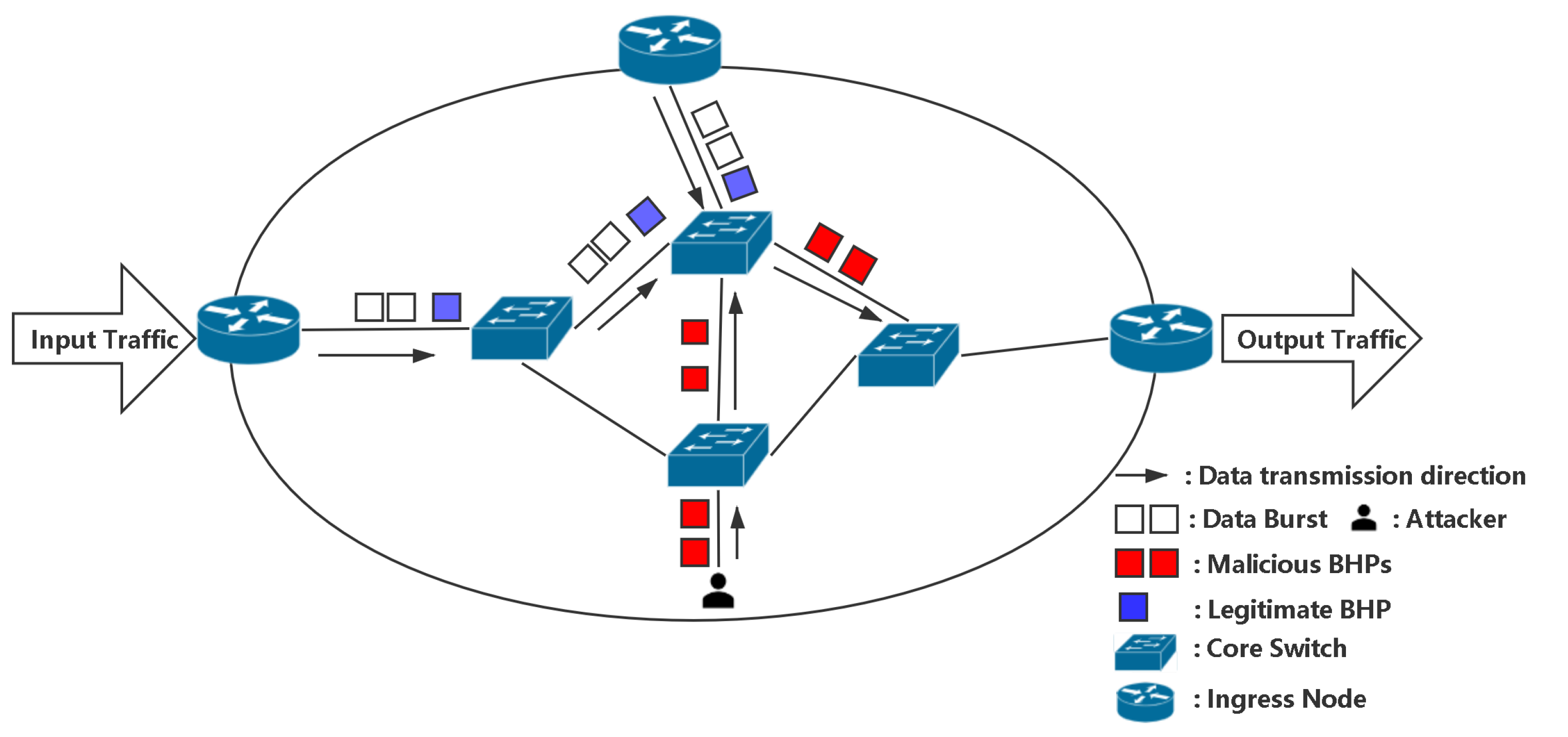
2.2. Problem Definition

When a malicious ingress node sends a large number of BHPs to the network, these BHPs occupy the core switch and take up the channel resources of the next DB. However, if the malicious node does not continue to send DB, then this will cause a large amount of reserved channel resources to be wasted, so that the normal BHP request has no available remaining channels, and the arriving DB afterward will also be discarded by the core switch. In this paper, our approach classifies the nodes based on the DB. We define three types of node status behaving, not behaving, and potentially not behaving, and four categories of nodes Block, No Block (NB), NB-No Block, NB-Wait. The semantics of the four categories are as follows: Block indicates that the node is in a blocking state due to improper traffic behavior. No Block indicates that the node is in a normal state. The remaining two values indicate that the node is in an intermediate state between Block and No Block, where the node is misbehaving but is below the threshold of Block. NB-No Block indicates that the node may be blocked soon. NB Wait indicates that the priority of node traffic and reservation is lower than other requests.

The definition of the classification problem is as following: The initial data is labelled as $\left(X,Y\right)$, where X represents the attribute set of each sample data, $Y$ represents the class variable. A vector $x_i\in R^m$ can be assigned one of four disjoint point sets $y_1$, $y_2$, $y_3$ or $y_4$ within an m-dimensional feature space. $x_i\in R^m$ is the ith training data row and $y_i\in \{0,1,2,3\}$ represents the ith class value. The aim is to derive a function, F, that maximizes the chance that $F\left(x\right)=y_i$ for each test data, $y_i$ can be 0 (NB-No Block), 1 (Block), 2 (No Block), 3 (NB-Wait). The function $F\left(x\right)$ can be defined as:

$$F\left(x\right)=y_i=\left\{\begin{array}{c}0,\mathrm{if}x\in C_0\hfill \\ 1,\mathrm{if}x\in C_1\hfill \\ 2,\mathrm{if}x\in C_2\hfill \\ 3,\mathrm{if}x\in C_3\hfill \end{array}\right.$$

(1)

2.3. Packet Data

The lack of data makes the detection of machine learning in the OBS network difficult. We perform a number of simulations to collect a relevant credible dataset, so that construct an effective classification model to block the BHP flooding attack. We randomly select 22 attributes of the data and have a brief description, as shown in

Table 1. Packet data attributes.

Label	Attribute	Description
D1	Node	The label of the sending node.
D2	Utilized Bandwidth Rate	Normalize the bandwidth rate that can be reserved.
D3	Packet Drop Rate	The ratio of the number of lost packets per node to the data sent.
D4	Full Bandwidth	This is the initially reserved bandwidth allocated by the user to each node.
D5	Average Delay Time Per Sec	This is the average delay of each node per second.
D6	Percentage Of Lost Packet Rate	Percentage of packet loss per node.
D7	Percentage Of Lost Byte Rate	Byte loss rate per node.
D8	Packet Received Rate	The number of data packets received by each node per second on the reserved bandwidth.
D9	Used Bandwidth	The amount of bandwidth that each node can use in the allocated bandwidth (D4).
D10	Lost Bandwidth	The amount of bandwidth lost by each node in the allocated bandwidth (D4).
D11	Packet Size Byte	The byte packet size allocated for each node.
D12	Packet Transmitted	The total number of data packets transmitted by each node per second in the allocated bandwidth (D4).
D13	Packet Received	The total number of packets received by each node per second in the allocated bandwidth (D4).
D14	Packet Lost	The total number of packets lost per second per node in the lost bandwidth (D10).
D15	Transmitted Byte	Bytes transferred per second per node.
D16	Received Byte	Number of bytes received by each node per second in the reserved bandwidth.
D17	10-Run-AVG-Drop-Rate	The average value of the packet loss rate (D3) obtained after 10 simulation runs.
D18	10-Run-AVG-Bandwidth-Use	The average value of used bandwidth (D9) obtained after 10 simulation runs.
D19	10-Run-Delay	The average delay time obtained after 10 simulation runs.
D20	Node Status	Divide node status into behaving, not behaving, and potentially not behaving.
D21	Flood Status	Flood rate of each node.
D22	Class	Four categories of nodes, Block, No Block (NB), NB-No Block, NB-Wait.

. We followed the feature selection process of Reference [9] (the source of this public dataset). The selection of features in the realm of interaction between optical networks and machine learning may also be found in References [16,17,18].

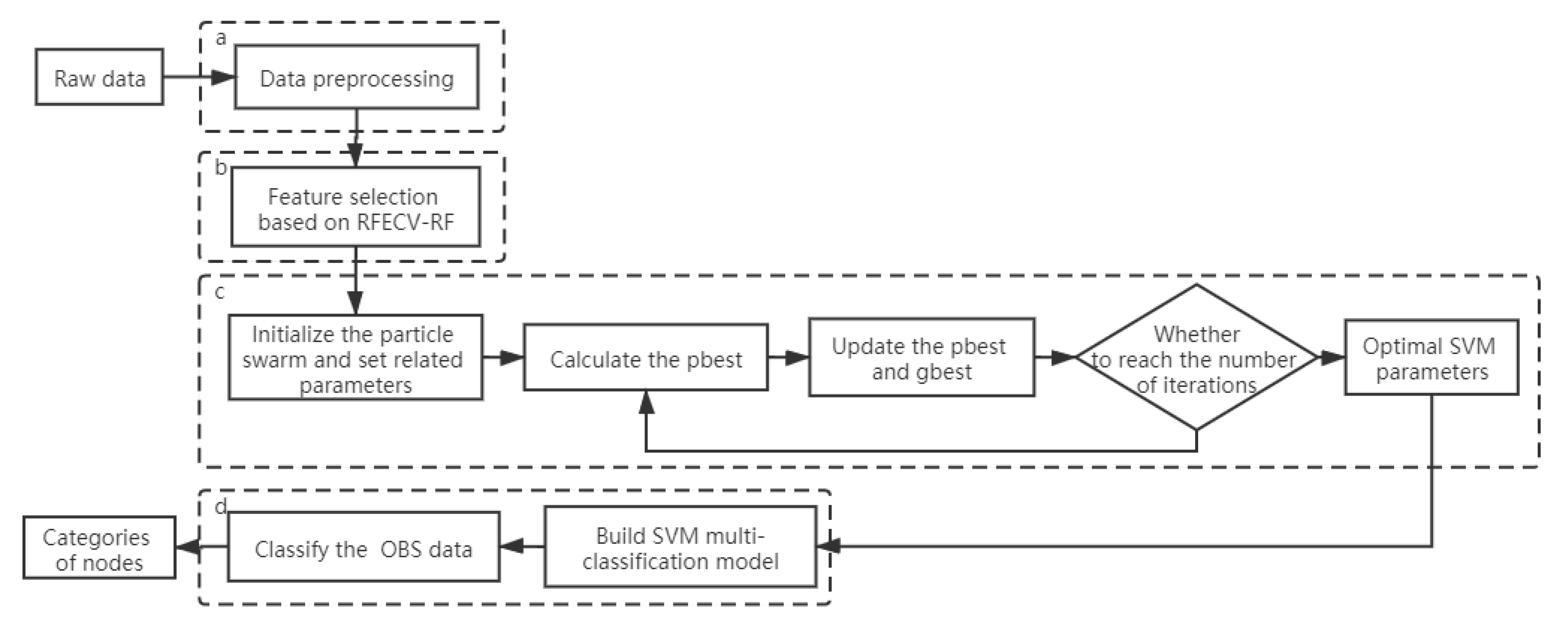
3. The Proposed PSO-SVM Model for the BHP Flooding Attack

We propose a BHP flooding attack detection framework based on PSO-SVM algorithm, which is divided into four modules, the brief description is as follows. Figure 2 represents the general architecture of PSO-SVM.

• Data preprocessing. The data is preprocessed accordingly so that our model can recognize it.
• Feature selection. Feature selection is performed on the data using RFECV-RF to find the most suitable subset of data for model classification based on classification accuracy values and cross-validation. The optimal feature set is segmented for model training and testing.
• Parameter tuning. PSO is introduced to find the two parameters of the given SVM model by finding the optimal combination of parameters.
• The OBS network intrusion detection model. The best combination of parameters is input to train the data, the trained model is tested against the test set, output the predicted result, and use the evaluation indexes, confusion matrix, etc. to evaluate the PSO-SVM model.

3.1. Data Preprocessing

To make the data more conducive to the analysis and learning of the model, we first perform the data processing procedure. In the real world, the initial data is generally incomplete, which is called “dirty data”. Learning directly from these data may lead to some errors. Data preprocessing is to convert “dirty data” into a form that can be “learned” by machine language. In particular, we perform the following data processing procedure:

Data cleaning: The data contains a small number of missing values and we remove the missing values, but this does not affect the model results. We also remove the Packet Size Byte (D11), because this attribute value is constant and does not provide any useful information.

Data transformation: To better process the attribute data, we convert the four categories NB NoBlock, Block, No Block, NB Wait and the node status behaving, not behaving, potentially not behaving into one-hot encoding, which makes the classifier more efficient in processing attribute data, and also expands the attribute characteristics in a certain function. The N-bit status register corresponds to N states, and each state is controlled by its independent register bit, and at any time, only one of the encoding is valid. For example, one-hot encoding of the ‘Node Status’ such as ‘NB, B, P NB’ are {1,0,0}, {0,1,0}, {0,0,1}.

After the above category transformation, all our data are converted into numeric. To eliminate the dimensional influence between data features, we need to normalize the features so that different indicators are comparable. We adopt the min-max normalization for data standardization processing, which can not only eliminate the influence of different attributes of samples with different orders of magnitude but also accelerate the search speed of the optimal solution of gradient descent and improve the classification accuracy.

$$X_{norm}=\frac{X-X_{min}}{X_{max}-X_{min}}$$

(2)

Equation (2) is the min-max normalized solution method, where $X_{\mathrm{norm}}$ is the normalized value, and $X_{\max }$ and $X_{\min }$ are the maximum and minimum values of the data before normalization. This approach compresses the data to the interval [0, 1] and outputs a value that is equal in proportion to the original value.

Data noise addition: To increase the statistical significance of the variables and smooth their values, Gaussian distribution is used to add noise to the data. It is also to prevent overfitting during model training.

$$\rho \left(z\right)=\frac{1}{\sqrt{2\pi \sigma }}exp\left\{-{(z-\mu )}^2/2{\sigma }^2\right\}$$

(3)

Equation (3) is the formula for the normal distribution, where $\pi$, $\sigma$ are the expectation and variance of the Gaussian distribution, respectively.

3.2. Feature Selection

As can be seen from Section 3.1, we have already preprocessed the data, but it is not at all sufficient to do this alone. The training results of the model will also be affected by the amount of data, the number of features, etc. For example, if all the features of the data are input into the model when training the model, there is a possibility that the model will be overfed. The feature values of some data do not affect the computational results of the model and may add some unnecessary computation. From the above, we should eliminate irrelevant features in the data as much as possible to ensure that the model training can get better results.

In this paper, we choose the RFE with K-fold Cross-Validation based on Random Forest (RFECV-RF) for feature selection [19]. The purpose of RFECV is to judge the optimal number of feature selections through a certain evaluation parameter. The steps of selection consist of two main phases: RFE and cross-validation, shown as Supplementary Materials Algorithm S1.

The external estimator uses the RF to obtain the corresponding feature importance order, i.e., the weight values [20]. Simply explained, feature importance is the average over the entire forest after counting the ‘contribution’ made by each feature on each tree. It is evaluated to find the features that are highly correlated with the targeted node state. In this paper, we use the Gini index to evaluate it, which is calculated as

$$G{I}_a=\sum _{y=0}^4\sum _{y^{\prime }\ne k}{p}_{ya}{p}_{y^{\prime }a}=1-\sum _{y=0}^4{p}_{ya}^2$$

(4)

where $p_{ya}$ represents the proportion of class y in the node a. The Gini index measures the probability that two samples are randomly selected from node a with different class. We will discuss the feature importance in Section 4.3.1.

The RFECV-RF algorithm performs feature selection on OBS network data by assigning a weight value to each feature. The features with the fewest absolute values are then deleted, and the remaining features are cycled through again. Adjusting the score of each feature during the iterative process to finally obtain the optimal feature subset. The time complexity of feature selection (RFECV-RF) is $O(mnlogn)+O\left(n^2\right)$ in the training phase.

3.3. Support Vector Machine

In this part, we introduce the Support Vector Machine (SVM) used for classification. Then, the optimization method of SVM, i.e., particle swarm optimization (PSO) algorithm, is proposed in Section 3.4.

SVM is a linear two-class classifier whose purpose is to find the maximum distance between categories and construct a classification hyperplane at the center of the maximum distance [21,22]. These two categories are labeled +1 (positive example) for the case above the hyperplane, and −1 (negative example) for the case below the hyperplane. The hyperplane can be expressed as:

$$y\left(x\right)={\alpha }^T\ast x+\beta$$

(5)

where $\beta$ denotes the deviation, $\alpha$ denotes the weight vector. $\alpha$ and $\beta$ can be estimated by minimizing the error function:

$$\begin{array}{c}{\displaystyle \underset{w,b,\xi >0}{min}}\frac{1}{2}{\alpha }^T\alpha +\mathcal{C}{\displaystyle \sum _i}{\xi }_i\\ \mathrm{s}.\mathrm{t}.y_i\left({\alpha }^T{x}_i+\beta \right)\ge 1-{\xi }_i,i=1,\dots ,n\\ {\xi }_i\ge 0\end{array}$$

(6)

where $\alpha$ is the slack variable and $\mathcal{C}$ is penalty parameter.

To predict to which classification the new records should be classified, the features of the new data are subsequently used. Once the decision-making surface is reached, the new data can be classified. Since there are four types of centralized attacks on OBS network data, we use One-Versus-Other (OVR) to create a multi-classified SVM. OVR employs four SVMs, each of which determines if a sample belongs to a specific category.

To solve linearly indivisible data, SVM transfers data that cannot be partitioned in low-dimensional feature space into higher-dimensional space for partitioning and employs kernel functions to calculate the inner product. The commonly used kernel functions are linear kernel, polynomial kernel, Radial Basis Function (RBF) kernel, and sigmoid kernel. Each kernel function has its own set of circumstances that is used. The majority of users base their decisions on previous experience. In this paper, we choose to use the RBF kernel with a short running time and the highest classificationaccuracy. The formula for RBF is:

$$K\left(x_1,x_2\right)=exp\left(-\frac{{∥x_1-x_2∥}^2}{2{\sigma }^2}\right)$$

(7)

where $\sigma$ is the width of RBF. The hyperplane is updated as:

$$\begin{array}{c}y\left(x\right)={\alpha }^T\ast K\left(x_1,x_2\right)+\beta \\ x\in D_{xi}\end{array}$$

(8)

where $\beta$ denotes the deviation, $\alpha$ denotes the weight vector, and $D_{xi}$ is the optimal feature subset.

3.4. Optimization of the SVM by PSO

From above, we selected the RBF kernel function. The RBF parameter $\sigma$ and the penalty parameter $\mathcal{C}$, among the many parameters of SVM, plays a critical role in the quality of the classification results. As the width value of the RBF, $\sigma$ directly determines the radial range of action of the kernel function, and the generalization ability of the model increases as $\sigma$ becomes larger, but declines after a certain value. The penalty factor is used to control the minimum risk and confidence level. Similarly, a smaller $\mathcal{C}$ reduces the model’s complexity, implying a smaller penalty for incorrect samples, while a larger $\mathcal{C}$ leads to overfitting.

We introduce the PSO algorithm to adjust the parameters of SVM [21,22]. Each member of the group is regarded by PSO as a “particle”, which moves at a set speed within its search range. All particles have the attributes of position, speed, and memory function. The fitness function is used to calculate the fitness value to judge the particle’s current position. Through the individual “notification” function, the particles follow the optimal particle within the scope of the search until the set number of iterations is reached or the optimal solution of the group no longer changes. The most common particles are known as the best position experienced by the individual particle (pbest) and the best position experienced by the population (gbest). The structure of PSO is given in Supplementary Materials Algorithm S2. The time complexity of PSO-SVM is $O\left(n^2\right)\times [O\left(m^2\times n\right),O\left(m^3\times n\right)]$ in the training phase. After being well-trained, only the classifier SVM is working, reducing the time complexity.

4. Experiments and Results

4.1. Experimental Settings

4.1.1. Dataset

We perform a number of simulations to collect a relevant credible dataset, so that construct an effective classification model to block the BHP flooding attack. We have obtained a relevant credible dataset in the UCI database [23]. There are 1075 sample data and each sample data contains 22 attributes. Our training dataset accounts for 80%, and the test dataset accounts for 20%.

The simulated OBS network constructs of one legitimate sender, one receiver, one attacker, eight core switches, two ingress edge routers, one egress edge router. This attacker is deployed close to this receiver in addition to the possibility of not being discovered. Every four core switches form a ring topology and are then connected in series. This dataset was obtained by running the NSFNET network structure over 100 simulations on NCENTs simulation platform, randomly selecting the locations of edge routers and varying the bandwidth capacity of the edge nodes (the network bandwidth takes values between (100–1000 Mbps)) to ensure that there is normal, contention and congestion in the network [24] (please see paper [9] for more details).

For illustration purposes,

Table 2. Partial dataset (Part I).

D1	D2	D3	D4	D5	D6	D7	D8	D9	D10	D11
3	0.623081	0.387489	200	0.000426	38.715738	38.748895	0.612511	124.61625	75.38375	1440
9	0.861525	0.151567	500	0.000961	15.152253	15.156679	0.848433	430.7625	69.2375	1440
3	0.559238	0.450597	100	0.000704	44.993369	45.059682	0.549403	55.92375	44.07625	1440
9	0.867038	0.146063	1000	0.000633	14.598556	14.606306	0.853937	867.0375	132.9625	1440
3	0.262688	0.741437	300	0.000473	74.103056	74.143659	0.258563	78.80625	221.19375	1440
9	0.542763	0.465611	900	0.000406	46.55864	46.5611	0.534389	488.48625	411.51375	1440

and

Table 3. Partial dataset (Part II).

D12	D13	D14	D15	D16	D17	D18	D19	D20	D21	D22
18,096	11,084	7012	2.605824 × 10${}^7$	1.59096 × 10${}^7$	0.290617	0.560773	0.000422	P NB	0.063936	NB-No Block
45,188	38,339	6849	6.507072 × 10${}^7$	5.520816 × 10${}^7$	0.103065	0.85291	0.000913	B	0	No Block
9048	4971	4077	1.302912 × 10${}^7$	7,158,240	0.3019	0.492129	0.000683	P NB	0.06038	NB-No Block
90,324	77,131	13,193	1.3006656 × 10${}^8$	1.1106864 × 10${}^8$	0.091862	0.841026	0.000627	B	0	No Block
27,092	7005	20,087	3.901248 × 10${}^7$	1.00872 × 10${}^7$	0.533834	0.225911	0.001336	NB	0.400376	Block
81,276	43,433	37,843	1.1703744 × 10${}^8$	6.254352 × 10${}^7$	0.35852	0.466776	0.00656	P NB	0.136238	NB-Wait

list just three iterations for two of the edge nodes.

4.1.2. PSO Experimental Setting

In the experiments, we considered a SVM based on the RBF kernel. Finding the optimal $\sigma$ and $\mathcal{C}$ for the SVM model to classify the OBS network dataset is a crucial step. The parameter tuning module consists of 100 particles and optimizes in 10 iterations. The related parameters $\sigma$ and $\mathcal{C}$ range randomly in [0.01, 10], [0.01, 100], respectively.

Table 4. SVM optimization parameters.

Parameters	Values
Population iterations	10
Population size	100
Local learning factor	0.2
Global learning factor	0.5
Inertia weight	0.5
Penalty factor	0.01 < $\mathcal{C}$ <100
Kernel function parameter	0.01 < $\sigma$ <10

shows the parameters empirically set by the PSO algorithm for SVM optimization search.

4.1.3. Evaluation Indexes

The confusion matrix, also known as the error matrix, is mostly used to judge the pros and cons of a classifier, which is suitable for a classified data model. The four basic indicators are obtained: True Positive (TP)—correct identification, False Positive (FP)—misidentification, True Negative (TN)—correct rejection, False Negative (FN)—false rejection. Furthermore, we extend the basic statistical results of the confusion matrix to the following four indexes: Accuracy, Precision, Recall, F1 score. The four evaluation indexes are defined in

Table 5. Four classification evaluation indexes.

Evaluation Index	Format
Accuracy	$(\mathrm{TP}+\mathrm{TN})/(\mathrm{TP}+\mathrm{FN}+\mathrm{FP}+\mathrm{TN})$
Precision	$\mathrm{TP}/(\mathrm{TP}+\mathrm{FP})$
Recall (TPR)	$\mathrm{TP}/(\mathrm{TP}+\mathrm{FN})$
F1 score	$2\times (\mathrm{Precision}\times \mathrm{Recall})/(\mathrm{Precision}+\mathrm{Recall})$

.

The Receiver Operating Characteristic (ROC) curve and Precision-Recall (PR) curve are also used in this paper to evaluate the classification effect of intrusion detection [25,26]. The ROC curve is a representation of the relationship between True Positive Rate (TPR) and False Positive Rate (FPR). The PR curve is a representation of the relationship between the accuracy rate and the recall rate. The formula for FPR are defined as

$$\mathrm{FPR}=\mathrm{FP}/(\mathrm{FP}+\mathrm{TN})$$

(9)

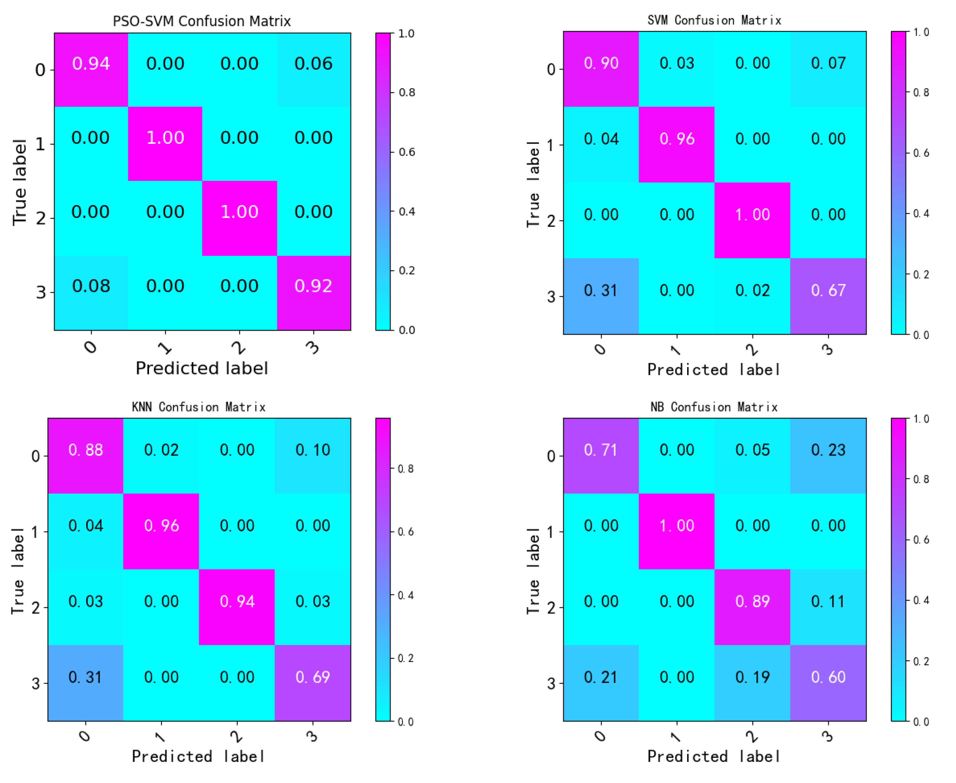
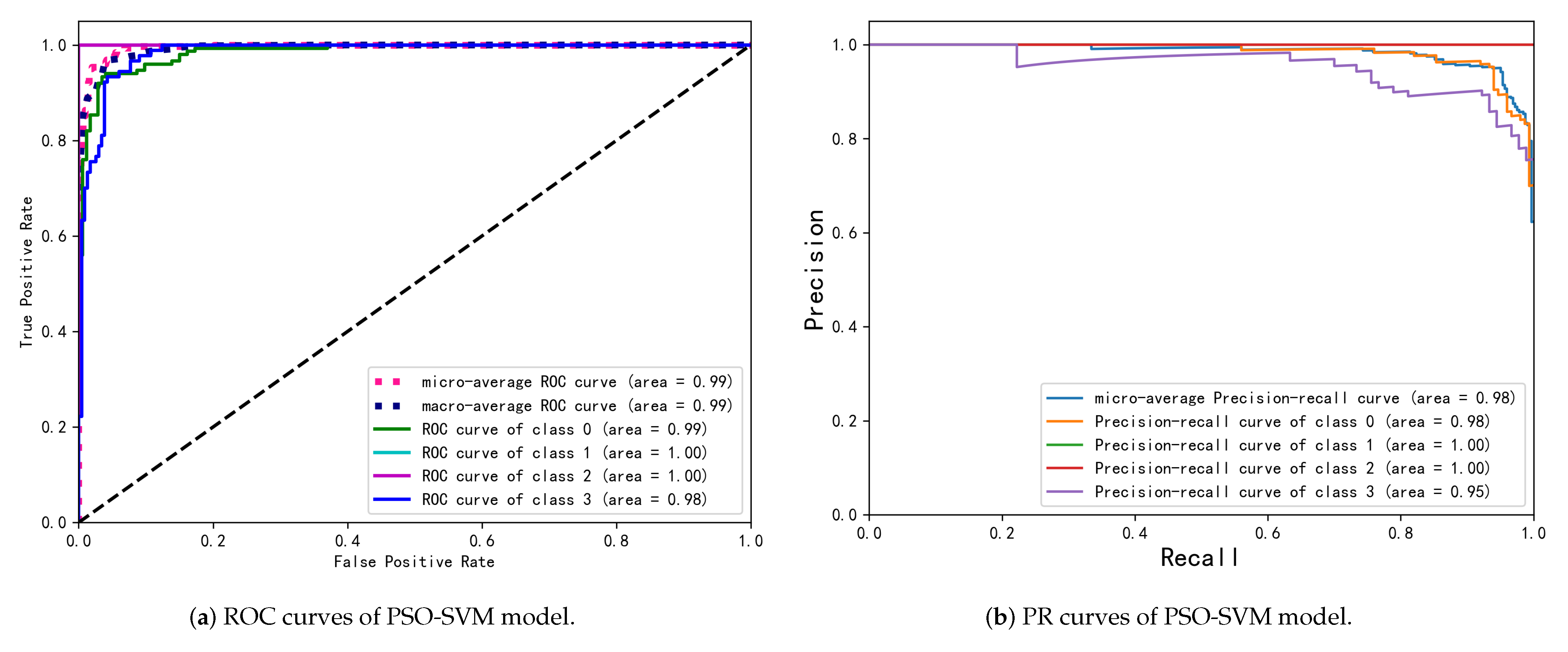
4.2. Experimental Results

The proposed PSO-SVM model is compared with the commonly used Naïve Bayes (NB), SVM, and k-Nearest Neighbor (KNN) models to detect the detection efficiency of BHP flooding attacks in the OBS network. Figure 3 shows the confusion matrix of the four algorithms. The PSO-SVM model has an accuracy of 100% for the second and third categories, and more than 90% for the two outer categories. The other three algorithms also have high accuracy for the second and third categories, but are not as effective for the other two categories. Among them, the NB algorithm has the worst effect, and the recognition accuracy of the fourth classification is only 60%. In a comprehensive view, the PSO-SVM algorithm has a strong advantage for detecting the BHP flooding attack in OBS networks. For comparison, we also present the specific values of the confusion matrix (Supplementary Materials Figure S1).

We also list the classification performance metrics of these four models, and two additional models, i.e., deep convolutional neural network (DCNN) [15] and decision tree (DT) [11], as shown in

Table 6. Performance index results of four models.

Models	Accuracy	Precision	Recall	F1 Score
PSO-SVM (our)	0.950	0.963	0.966	0.965
SVM	0.854	0.882	0.881	0.878
KNN	0.845	0.886	0.868	0.875
NB	0.743	0.748	0.800	0.763
DT [11]	0.87	0.593	0.574	0.583
DCNN [15]	0.99	0.99	0.99	0.99

. These two models used the same dataset as in this paper. Since PSO is introduced in this paper to find the optimal parameters of the SVM model ($\sigma$ = 3.14, $\mathcal{C}$ = 2.69), all the performance metrics of PSO-SVM are superior than those of the SVM model. Additionally, the accuracy of PSO-SVM is improved by about 9.4%, 9.6%, 20.7%, 8% compared with SVM, KNN, NB, and DT, respectively, which has a better classification effect and improves the precision to 96.3%.

The NB algorithm predicts the predicted samples in a straightforward and quick manner. However, since the NB model assumes that the attributes are independent of one another, this assumption is difficult to verify in our data set. When the number of attributes is great or the correlation between attributes is large, this results in a higher categorization of the NB model. When the KNN algorithm encounters sample imbalance, the prediction deviation is relatively substantial. For example, there are fewer samples in one category, whereas there are more samples in others. SVM algorithm’s low prediction accuracy is due to its sensitivity to missing data, the selections of parameters and kernel function, and lack of accuracy for multi-class prediction. Rajab et al. [11] chose only two features that were highly significant to the category in the decision tree, leaving out some information. In addition, the decision tree model does not train well enough for the categories with less samples in the dataset (NB-No Block and NB-Wait).

The convolutional layer in DCNN retrieves data features, which decreases the empirical error of manually extracting features. Compared with others, DCNN has a better classification effect including our model. However, the number of features obtained by DCNN is large, the processing time is long, and the training time is greatly increased.

The PR curve and the ROC curve are utilized in this paper to evaluate the classification effectiveness of our model. Figure 4a shows the ROC curves for each of the four categories, as well as the two calculation methods of micro-averaging (micro) and macro-averaging (macro). Our PSO-SVM model has a better classification impact, as the ROC regions of the four categories are infinitely close to 1. The PR curves for all four categories, as shown in Figure 4b, maintain a steady convexity to the right, indicating that the PSO-SVM model can maintain a very high prediction accuracy as the recall rate steadily increases. In conclusion, our PSO-SVM model provides a more accurate and efficient flooding attack detection approach.

4.3. Discussion

In this part, we consider the feature importance magnitude, the effect of two variables, the number of selected features in Section 3.2 and kernel function in Section 3.3, on our PSO-SVM detection model.

4.3.1. The Feature Selection

In REFCV, we employed a RF as an external estimator for feature selection. The importance of features computed with the Gini index in random forest is displayed in Figure 5a. We graded the feature importance from left to right in descending order. The differences in terms of values are not significant. ‘Flood Status’ has a greater impact on identifying flooding attacks than other aspects. ‘10-Run-AVG-Drop-Rate’ is the second most important. ‘10_Run_AVG_Bandwidth_Use’, ‘Percentage_Of_Lost_Byte_Rate’, ‘Packet_Drop_Rate’ and other values are roughly equal and are third important. The values of ‘10-Run-Delay’, ‘Used_Bandwidth’, and ‘Packet_Received’ are approximately equal, and again of. The remaining five are roughly equal and have very little impact. ‘Node status’ such as ‘NB, B, P NB’, on the other hand, has almost no influence.

We perform several experiments with the number of features ranging from 1 to 20 and compare their model accuracy. Figure 5b shows the variation of the accuracy of RFECV-RF in finding the optimal subset of features for the OBS network. It can be seen that as RFE repeatedly constructs the random forest model and uses 5-fold cross-validation for selection, the highest result score is achieved when the number of features is 15, and the best classification is achieved.

Meanwhile,

Table 7. Selected features I.

D1	D2	D3	D4	D5	D6	D7	D8	D9	D10
False	True	True	False	True	True	True	True	True	True

“True” under a certain feature represents this feature is selected, “False” represents it’s not.

and

Table 8. Selected features II.

D12	D13	D14	D15	D16	D17	D18	D19	D20	D21
False	True	True	False	True	True	True	True	False	True

“True” under a certain feature represents this feature is selected, “False” represents it’s not.

displays the 15 features that were picked. ‘True’ indicates that the corresponding feature is selected, whereas ‘False’ indicates that it is not. Meanwhile, the 15 features that were selected are shown in the table. The five eliminated features are ‘Node’, ‘Full Bandwidth’, ‘Packet Transmitted’, ‘Transmitted Byte’, and ‘Node Status’, corresponding to the five features with the lowest importance in Figure 5a.

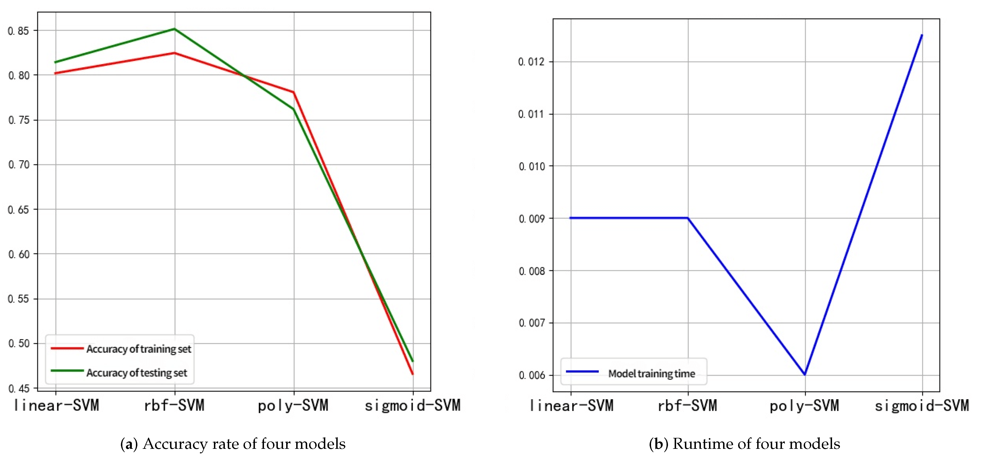
4.3.2. Kernel Function Selection

In this paper, we experimentally compare the effects of these four kernel functions linear kernel, polynomial kernel, Radial Basis Function (RBF) kernel, sigmoid kernel on the classification of the dataset in order to find the best kernel function for the classification of OBS network data. As shown in Figure 6, the choice of kernel function has a significant impact on the accuracy and training time of the model. The Sigmoid-SVM has the longest running time and the worst results, while Poly-SVM has a shorter time, but its classification accuracy is not high. Considering comprehensively, we choose to use the RBF kernel with a short running time and the highest classification accuracy.

5. Conclusions

With the increasing complexity of network data and the environment, the concealment and complexity of network intrusion have become stronger and stronger. Moreover, since network intrusion is not limited by time and space, once the attack occurs, it will cause great harm to network security. Therefore, it is very important to accurately detect intrusion data. In this paper, we propose an RFE-PSO-SVM model for intrusion detection in OBS networks, where RFE for feature extraction, PSO for finding the optimal combination parameters of SVM. Then, we test the model through the data obtained from the NCENTs simulation platform. The experimental results show that NB, SVM, and KNN all have overfitting problems, so the traditional machine learning model is difficult to classify the problems under different network attacks. The prediction accuracy of the PSO-SVM model is 9.4%, 9.6%, 20.7%, 8% higher than that of SVM, KNN, NB and DT. Although DCNN has a good effect, it takes a long time to train, and adding more network layers causes gradient dispersion and explosion. Overall, our method considerably enhances BHP flooding attack detection in OBS networks, with significant and high-efficiency classification.

References

1. Qiao, C.; Yoo, M. Optical burst switching (OBS)—A new paradigm for an Optical Internet. J. High Speed Netw. 1999, 8, 69–84. [Google Scholar]
2. Al-Shargabi, M.A.; Shaikh, A.; Ismail, A.S. Enhancing the quality of service for real time traffic over Optical Burst Switching (OBS) networks with ensuring the fairness for other traffics. PLoS ONE 2016, 11, e0161873. [Google Scholar] [CrossRef] [PubMed] [Green Version]
3. Dumych, S. Study on traffic aggregation algorithms for edge nodes of optical burst switching network. In Proceedings of the 2016 13th International Conference on Modern Problems of Radio Engineering, Telecommunications and Computer Science (TCSET), Lviv, Ukraine, 23–26 February 2016; pp. 947–949. [Google Scholar]
4. Oh, S.Y.; Hong, H.H.; Kang, M. A data burst assembly algorithm in optical burst switching networks. Etri J. 2002, 24, 311–322. [Google Scholar] [CrossRef]
5. Sliti, M.; Hamdi, M.; Boudriga, N. A novel optical firewall architecture for burst switched networks. In Proceedings of the 2010 12th International Conference on Transparent Optical Networks, Munich, Germany, 27 June–1 July 2010; pp. 1–5. [Google Scholar]
6. Sliti, M.; Boudriga, N. BHP flooding vulnerability and countermeasure. Photonic Netw. Commun. 2015, 29, 198–213. [Google Scholar] [CrossRef]
7. Sreenath, N.; Muthuraj, K.; Kuzhandaivelu, G.V. Threats and vulnerabilities on TCP/OBS networks. In Proceedings of the 2012 International Conference on Computer Communication and Informatics, Coimbatore, India, 10–12 January 2012; pp. 1–5. [Google Scholar]
8. Eddy, W. TCP SYN Flooding Attacks and Common Mitigations. Technical Report, RFC 4987. 2007. Available online: http://www.rfc-editor.org/info/rfc4987 (accessed on 1 June 2021). [CrossRef] [Green Version]
9. Rajab, A.; Huang, C.T.; Al-Shargabi, M.; Cobb, J. Countering burst header packet flooding attack in optical burst switching network. In International Conference on Information Security Practice and Experience; Springer: Berlin/Heidelberg, Germany, 2016; pp. 315–329. [Google Scholar]
10. Coulibaly, Y.; Al-Kilany, A.A.I.; Abd Latiff, M.S.; Rouskas, G.; Mandala, S.; Razzaque, M.A. Secure burst control packet scheme for Optical Burst Switching networks. In Proceedings of the 2015 IEEE International Broadband and Photonics Conference (IBP), Bali, Indonesia, 23–25 April 2015; pp. 86–91. [Google Scholar]
11. Rajab, A.; Huang, C.T.; Al-Shargabi, M. Decision tree rule learning approach to counter burst header packet flooding attack in optical burst switching network. Opt. Switch. Netw. 2018, 29, 15–26. [Google Scholar] [CrossRef]
12. Jayaraj, A.; Venkatesh, T.; Murthy, C.S.R. Loss classification in optical burst switching networks using machine learning techniques: Improving the performance of tcp. IEEE J. Sel. Areas Commun. 2008, 26, 45–54. [Google Scholar] [CrossRef]
13. Mata, J.; de Miguel, I.; Duran, R.J.; Merayo, N.; Singh, S.K.; Jukan, A.; Chamania, M. Artificial intelligence (AI) methods in optical networks: A comprehensive survey. Opt. Switch. Netw. 2018, 28, 43–57. [Google Scholar] [CrossRef]
14. Ibrahim, L.M. Anomaly network intrusion detection system based on distributed time-delay neural network (DTDNN). J. Eng. Sci. Technol. 2010, 5, 457–471. [Google Scholar]
15. Hasan, M.Z.; Hasan, K.Z.; Sattar, A. Burst header packet flood detection in optical burst switching network using deep learning model. Procedia Comput. Sci. 2018, 143, 970–977. [Google Scholar] [CrossRef]
16. Boutaba, R.; Salahuddin, M.A.; Limam, N.; Ayoubi, S.; Shahriar, N.; Estrada-Solano, F.; Caicedo, O.M. A comprehensive survey on machine learning for networking: Evolution, applications and research opportunities. J. Internet Serv. Appl. 2018, 9, 16. [Google Scholar] [CrossRef] [Green Version]
17. De Sanctis, M.; Bisio, I.; Araniti, G. Data mining algorithms for communication networks control: Concepts, survey and guidelines. IEEE Netw. 2016, 30, 24–29. [Google Scholar] [CrossRef]
18. Gu, R.; Yang, Z.; Ji, Y. Machine learning for intelligent optical networks: A comprehensive survey. J. Netw. Comput. Appl. 2020, 157, 102576. [Google Scholar] [CrossRef] [Green Version]
19. Wang, C.; Pan, Y.; Chen, J.; Ouyang, Y.; Rao, J.; Jiang, Q. Indicator element selection and geochemical anomaly mapping using recursive feature elimination and random forest methods in the Jingdezhen region of Jiangxi Province, South China. Appl. Geochem. 2020, 122, 104760. [Google Scholar] [CrossRef]
20. Li, X.; Chen, W.; Zhang, Q.; Wu, L. Building auto-encoder intrusion detection system based on random forest feature selection. Comput. Secur. 2020, 95, 101851. [Google Scholar] [CrossRef]
21. Hu, J.; Zeng, J.; Wei, L.; Yan, F. Improving the Diagnosis Accuracy of Hydrothermal Aging Degree of V2O5/WO3–TiO2 Catalyst in SCR Control System Using an GS–PSO–SVM Algorithm. Sustainability 2017, 9, 611. [Google Scholar] [CrossRef] [Green Version]
22. Du, J.; Liu, Y.; Yu, Y.; Yan, W. A prediction of precipitation data based on support vector machine and particle swarm optimization (PSO-SVM) algorithms. Algorithms 2017, 10, 57. [Google Scholar] [CrossRef]
23. Rajab, A. Burst Header Packet (BHP) Flooding Attack on Optical Burst Switching (OBS) Network Data Set. University of California Irvine Data Repository. 2017. Available online: https://archive.ics.uci.edu/ml/datasets/Burst+Header+Packet+%28BHP%29+flooding+attack+on+Optical+Burst+Switching+%28OBS%29+Network (accessed on 1 June 2021).
24. National Chiao Tung University. NCTUns. Available online: http://nsl.csie.nctu.edu.tw/nctuns.html (accessed on 1 June 2021).
25. Fawcett, T. An introduction to ROC analysis. Pattern Recognit. Lett. 2006, 27, 861–874. [Google Scholar] [CrossRef]
26. Davis, J.; Goadrich, M. The relationship between Precision-Recall and ROC curves. In Proceedings of the 23rd International Conference on Machine Learning, Pittsburgh, PA, USA, 25–29 June 2006; pp. 233–240. [Google Scholar]
Figure 1. BHP flooding attacks in an OBS network.
Photonics 08 00555 g001
Figure 2. Architecture of the proposed PSO-SVM model.
Photonics 08 00555 g002
Figure 3. Comparison of the confusion matrix (scale) of the four algorithms. 0∼3 indicate the 4 labels, respectively, 0: NB-No BlOCK, 1: BlOCK, 2: No BlOCK, and 3: NB WAIT.
Photonics 08 00555 g003
Figure 4. Comparison of different kernel function models for SVM in optical interconnect data.
Photonics 08 00555 g004
Figure 5. (a) Feature importance values in descending order, from left to right. (b) Schematic diagram of optimal feature subset selection.
Photonics 08 00555 g005
Figure 6. Comparison of different kernel function models for SVM in optical interconnect data.
Photonics 08 00555 g006