Article

Evaluation of Three Iterative Algorithms for Phase Modulation Regarding Their Application in Concentrating Light Inside Biological Tissues for Laser Induced Photothermal Therapy

1
Departamento de Física, Faculdade de Ciências e Tecnologia, Universidade Nova de Lisboa, 2825-149 Monte da Caparica, Portugal
2
Instituto de Biofísica e Engenharia Biomédica, Faculdade de Ciências, Universidade de Lisboa, Campo Grande, 1749-016 Lisboa, Portugal
*
Author to whom correspondence should be addressed.
Photonics 2021, 8(9), 355; https://doi.org/10.3390/photonics8090355
Submission received: 26 July 2021 / Revised: 23 August 2021 / Accepted: 25 August 2021 / Published: 27 August 2021
(This article belongs to the Special Issue Tissue Optics)

Abstract

:
The focusing of light through turbid media like biological tissues is strongly hindered by the scattering of light which limits its safe practice and application in medicine. In order to control this phenomenon, we shaped the incident wavefront using three algorithms including a four-element division algorithm, a partitioning algorithm, and simulated annealing to control, iteratively, a spatial light modulator (SLM). We have tested two different convergence criteria to achieve a focal point inside a turbid environment, made up of a mixture of agar and milk, set to mimic a specific depth of human skin, and provide comparison results. A camera and a lens are used to visualize the focal area and give feedback information to the algorithms. A discussion on the use of these algorithms and convergence criteria is presented, being focused on its convergence time and performance. Depending on the algorithm and operational parameters, improvements of 29% to 46% of the irradiance in the region of interest were accomplished.

1. Introduction

The development of new diagnostic and treatment techniques that are more efficient and less invasive so that the damage of healthy tissue can be minimized is of major importance in medicine. For this matter, the interaction of laser radiation with biological tissue has been the target of great attention with one of its applications being phototherapy. In addition to this application, drug delivering nanoparticles have been studied [1,2] where the rise in temperature allows for the remote release of drugs contained in it into the biological system. Due to its destructive effect over malignant tissues, like cancer cells, this has already been used in some superficial skin cancer treatments [3]. Despite this latter success, it is of interest that this application can be expanded to the point of acting in regions that surpass the surface of the skin, with its thickness ranging from 0.6 mm to 3.2 mm [4], where the turbid nature of tissues prevents the laser from delivering the necessary dose in destroying the undesired tissues. In addition, this expansion requires the consideration of not compromising the health of the surrounding cells. The dose, in this case, can also be referred to as energy density, whose values can be known for the destruction of tumoral tissues [5], and it is associated with the irradiance (I) and exposure time (texp) by the following expression:
D = I · t e x p = P A · t e x p ,
P being the laser power and A the area of the beam of the target.
In order to better target the tumor cells and protect the healthy surrounding cells, gold nanoparticles (GNP) have been studied [6,7]. These GNP are functionalized so they aggregate around tumors, and they have “tunable high-absorption properties in the NIR region that allow for local higher absorbed energy” [8]. This allows for them to be photo-induced in a determined wavelength to produce heat (through an effect called Surface Plasmon Resonance, SPR [9]) consequently leading to cytotoxic damage of the surrounding cells. The possibility of tuning their absorption peak in the NIR region turns out to be advantageous since this includes the commonly called therapeutical window of wavelengths, where there is less absorption by the main absorption agents of biological tissues (650–900 nm) [10].
Regarding the strong scattering effect that limits the propagation of light in a desired trajectory and conditions the in-depth energy density, there is the need for achieving greater irradiance values over a small, focused, area. Therefore, numerous studies have been conducted in order to control this effect of light propagation through diffusive media of which manipulation of the laser wavefront (wavefront shaping) has been proven successful [11,12]. The principle behind it is to collect the scattered light from the turbid environment and, based on it, manipulate the incident wavefront to compensate for the dispersion effects. These current strategies are found to be split into passive or active solutions. Regarding the passive solutions, self-reconstruction beams allow for the desired effect where Bessel beams are less susceptible to the diffusive character of the medium and its application is mainly in optical coherence tomography and microscopy [11]. About the active solutions, these can be based in direct feedback, beacon, or holography [13,14,15]. All of these techniques find themselves on many imaging applications [16], but direct feedback wavefront shaping has been evolving to tumor phototherapy and provides the advantage of making use of a much less complex optical setup when compared to the other ones.
In this work, we apply phase manipulation of the wavefront of the incident light by using a spatial light modulator (SLM) and a detector’s information serving as direct feedback, to concentrate 808 nm light inside a static turbid sample, mimicking the scattering properties of the human skin. By changing the phase map of the incident light, it can compensate for the scattering effects that decrease the quality of focus in an iterative way [17]. Decreasing this area allows for larger irradiance values, following Equation (1), which in an in-depth tumor phototherapy application combined with GNP will allow to manipulate, by knowing the necessary dose (energy density), both the laser power and its exposure time to a minimum. In an engineering insight, these encouraging abilities of direct feedback wavefront shaping can enable the construction of a device without recurring to a complex system with a powerful, expensive laser that has the potential of destroying superficial healthy tissues. This device would safely help in diagnosing and/or treating tumors.
The modulator (i.e., SLM) consists of a matrix of pixels that are grouped into an equal sized number of segments of which in this phase modulation technique are individually set to a phase map value, in between 0 and 2π. The multiple scattering of light inside a media can easily be associated as being a random and stochastic process along its path, yet it is considered a causal and reversible process over time [18]. In order to describe this phenomenon of light transport through a diffusive media, a transmission matrix allows to relate the incident and transmitted electric fields in the following way:
E m = n N t m n · E n = n N t m n · A n e i ϕ n .
Here, Em stands for the mth-channel of the transmitted electric field, tmn the element of the transmission matrix, En the nth-channel of the incident electric field, An the amplitude of the incident light from the nth-channel, and ϕn its phase. Considering that we are modulating the phase of the incident light by N segments, individually, while maintaining the amplitude constant, then ϕn will correspond to this modulated phase of incident light on a segment. This segmentation has proven useful in reducing the total number of iterations required in the optimization procedure but with a tradeoff: the lesser the number of segments, the lesser the enhancement potential. By considering a case of maximization of target intensity, the maximum theoretical enhancement factor η relates with the total number of segments N and target intensity before the optimization I 0 in the following way:
η = I m a x I 0 = N 1 π 4 + 1 ,
where the angle brackets denote ensemble averaging over disorder [19]. The control of the modulator is accomplished in testing three different optimization algorithms under two different evolution criteria (cost functions) in a fixed execution timespan, and we provide comparison results for all of these. Ultimately, we present our conclusions.

2. Phase Control Algorithms

The goal to achieve is to find an optimized wavefront by finding the phase mask that is applied to the incident light that results in the sharpest focus point inside the turbid media. The detector, being placed right outside of the media, will capture the transmitted intensity distribution where this focus point will be represented as a circular area which will be further called a spot area.
Feedback-based algorithms allow for an optimization procedure to take place in order to control the diffused light in a turbid medium while using a SLM in a simple optical setup. There are several algorithms that have been tested for wavefront modulation and they differ from each other by their runtime speed, enhancement factor, complexity, and stability in noisy environments. Since, in the medical context, we are interested in having a fast focus formation, due to the dynamic motion of tissues, the following explained algorithms were chosen because they have revealed good enhancement factors in a small number of iterations [20].

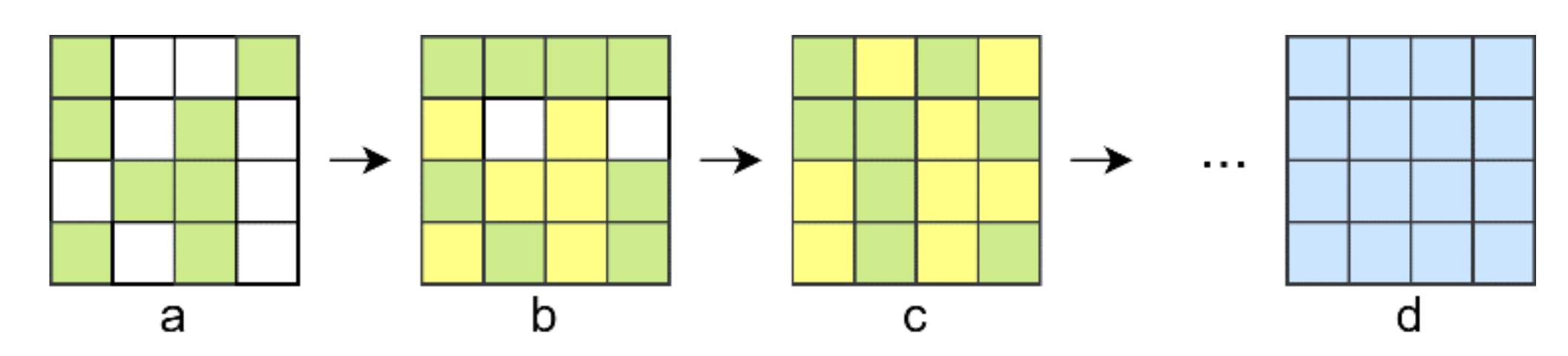
2.1. Four-Element Division Algorithm (FEDA)

This algorithm was firstly presented by Fang et al. [21] and the working principle behind it is by applying a two-by-two division of a square matrix so that it results in four matrices of equal size. Afterwards, the algorithm recursively acts on each of these resulting matrices originating new, smaller, matrices. The algorithm stops when its recursive action gives rise to divisions of a desired size. The optimization procedure to apply phase modulation starts by cycling the phase of the first segment as shown in Figure 1a from 0 to 2π in small phase steps. In each of these, an intensity image is acquired from the detector and a value for the chosen cost function is obtained. The phase at which this obtained value gets a maximum, or a minimum depending on the criteria, is then saved and set into this first segment before the optimization procedure continues. Afterwards, this procedure acts on the second segment while having the optimized segment value set for the first segment, as shown in Figure 1b, and an optimized value is then set. This operation takes place for the third and fourth segment until an optimized 2 × 2 format is obtained (Figure 1c–e). Next, one segment is then divided into four individual equal sized segments which are phase cycled as the previous ones but, first, they all inherit its previous optimized phase distribution, as depicted in Figure 1e. After finding an optimized phase value for one segment, this one is set to replace the inherited phase value before proceeding to the other small segment. This procedure can happen to turn an initial phase matrix into a 2 × 2 format which, recursively, turns into 4 × 4, 8 × 8, … optimized phase distribution formats. This process either ends until the number of segments equals the number of pixels of the SLM or until it reaches a desired format, whose total number of segments must be lower than the number of pixels.

2.2. Partitioning Algorithm (PA)

The Partitioning Algorithm technique finds an optimized wavefront by simultaneously acting on a whole group of segments and has been introduced in phase modulation techniques by Vellekoop et al. [22]. This optimization procedure starts by randomly selecting half of the total segments of an initial phase matrix and changing its phase values to random ones in the range of 0 to 2π. Afterwards, this disturbed phase matrix is projected on the SLM and a cost function value is calculated from the detector, by which, if it is better than the previous one, this new phase matrix is considered to be the best phase matrix. The algorithm proceeds by changing other random half segments of this best phase matrix to other random values, and this method is repeated, while receiving the detector feedback and changing; according to it, the current best phase matrix, until a chosen number of iterations has not been reached. Figure 2 illustrates the principle of this algorithm.

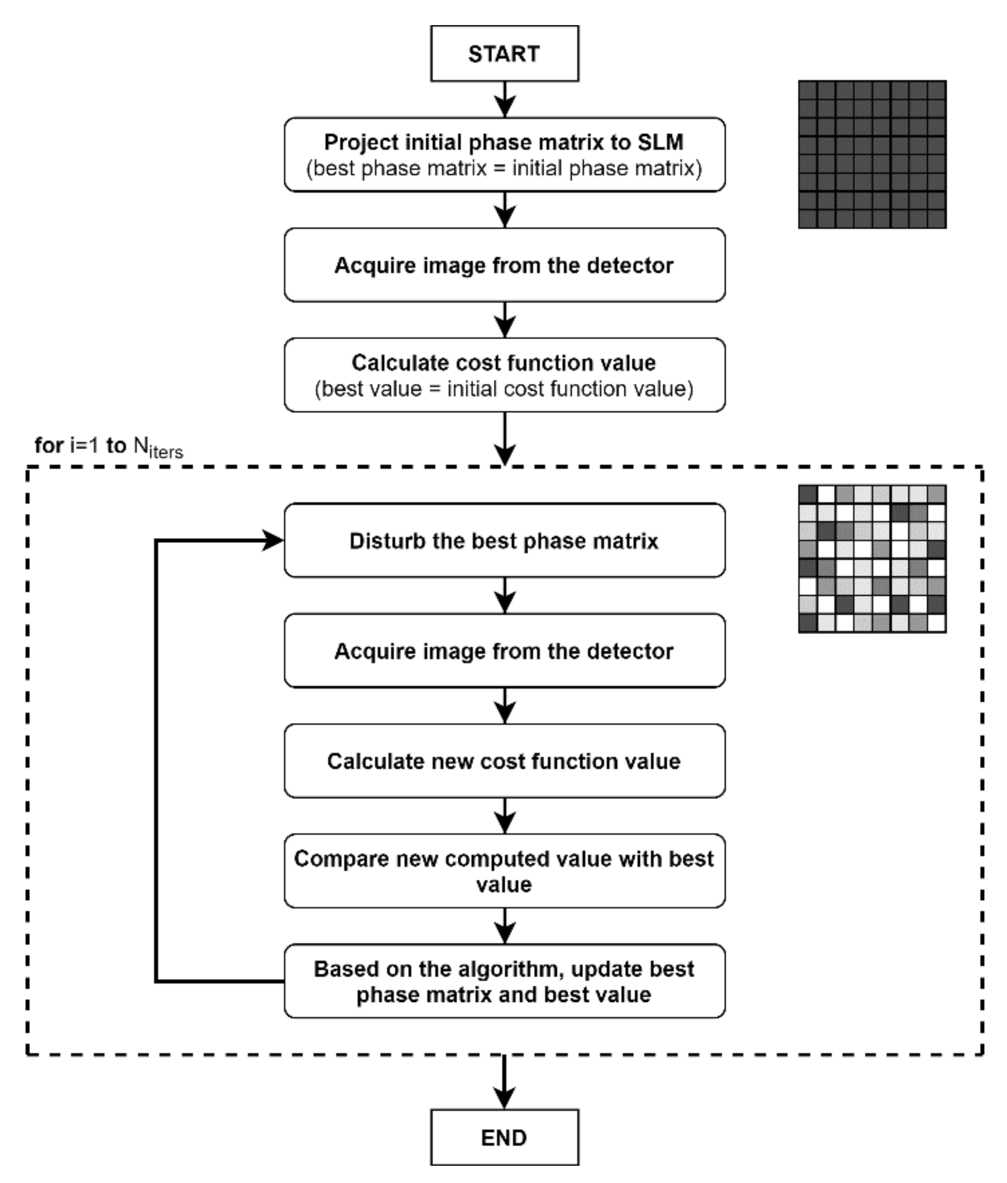
2.3. Simulated Annealing Algorithm (SAA)

The Simulated Annealing Algorithm is an optimization technique used to find a global optimum based on the simulation of the cooling of a metal in a heat bath—a process known as annealing. It works by simulating this cooling process by lowering the “temperature” of the system until it reaches a point where no change is observed (steady state). This technique is of interest due to its random character that allows to not get stuck with a local minimum, or maximum, peak [19,23]. The “temperature” is the core parameter of the SAA, being associated with the iteration number, and in the system, it decreases in the following way:
T k = α k T 0 , T 0 > 0 , k = 1 , 2 , 3 , ,
where Tk is the temperature of the kth iteration, T0 the initial temperature, and α (0 < α < 1) the decay factor. The scheme in Figure 3 shows the working principle of the SAA applied to the current study, and it starts by generating an initial temperature and sending an initial phase matrix to the SLM which is considered the first best. Afterwards, an intensity image is acquired from the detector and a value for the chosen cost function is calculated from it. Then, the algorithm enters a cycle of N iterations where at each iteration a disturbance is introduced over the best phase matrix. This consists of randomly selecting half of the number of total segments and changing its values to other random phase values. After that, a new value is calculated from the detector and, if this value is better than the previous best one, then the best phase matrix is replaced by this disturbed one. Otherwise, there is a chance of accepting a worse solution by giving it an acceptance probability, which is given by the Boltzmann function:
P T = e x p E o l d E n e w T , E o l d E n e w < 0 ,
where Eold and Enew correspond to the cost function values for the best phase matrix and current disturbed phase matrix, respectively, and T corresponds to the current temperature of the system. This happens for (EoldEnew) < 0 because the opposite case stands for the improvement situation, where the new perturbed phase matrix is better than the previous one. This way, one can see that this algorithm does its optimization procedure by achieving a minimum value of Enew, but, if a maximization is intended, then one can change these input parameters for their negative values. While the number of iterations has not reached the desired N value, the system continues to disturb the best phase matrix and accepting it according to the presented rule. After concluding the cycle, the temperature of the system is analyzed by comparing it with a given final temperature: if it is lower or equal, then the algorithm stops, but, if it is higher, then the temperature is lowered following Equation (4), where there is an increment in the k value. In this case, the perturbation on the best phase matrix continues to act iteratively, and this entire process is repeated until the current temperature of the system reaches the final temperature value or until a desired number of iterations is made.

2.4. Cost Functions

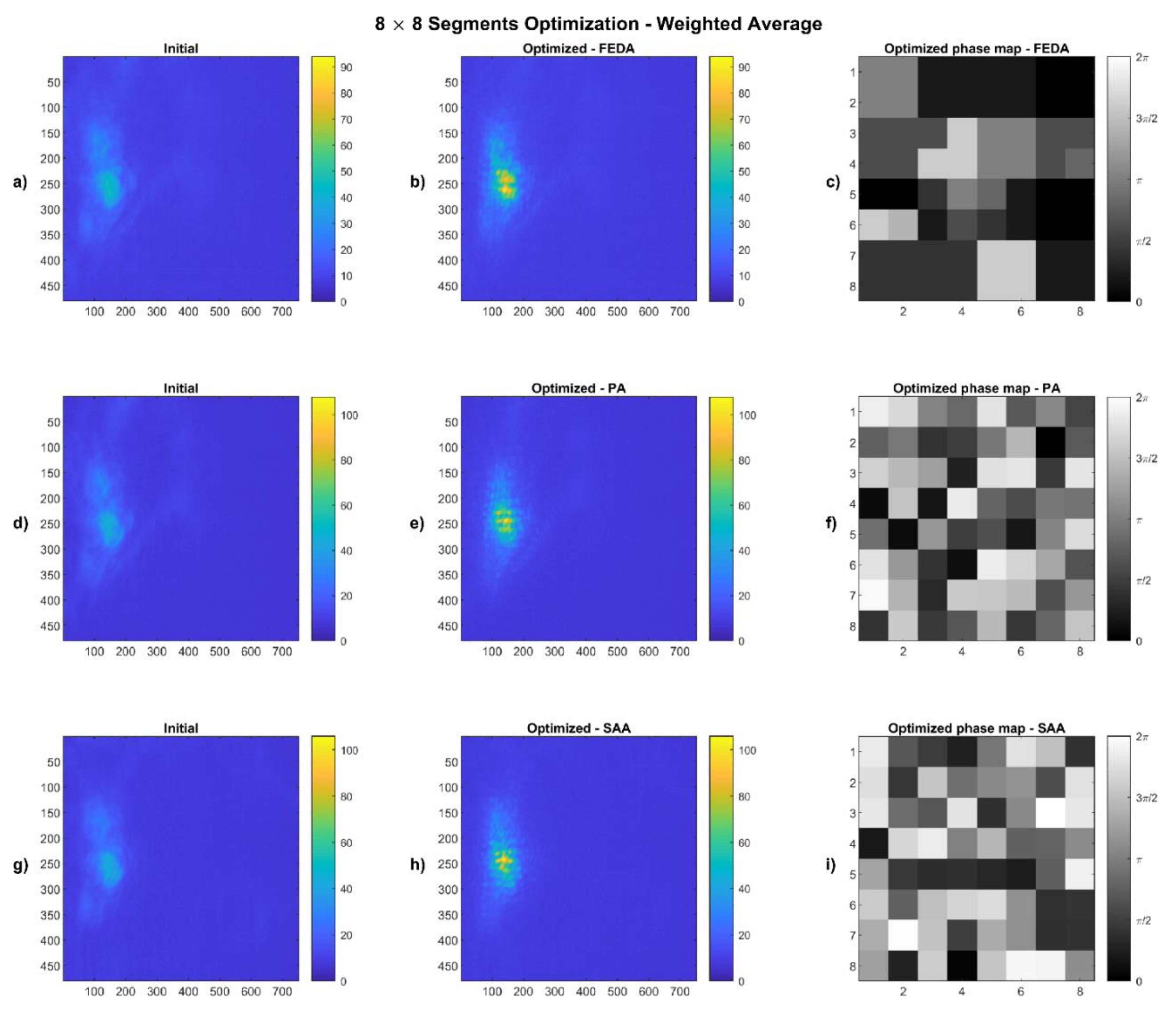
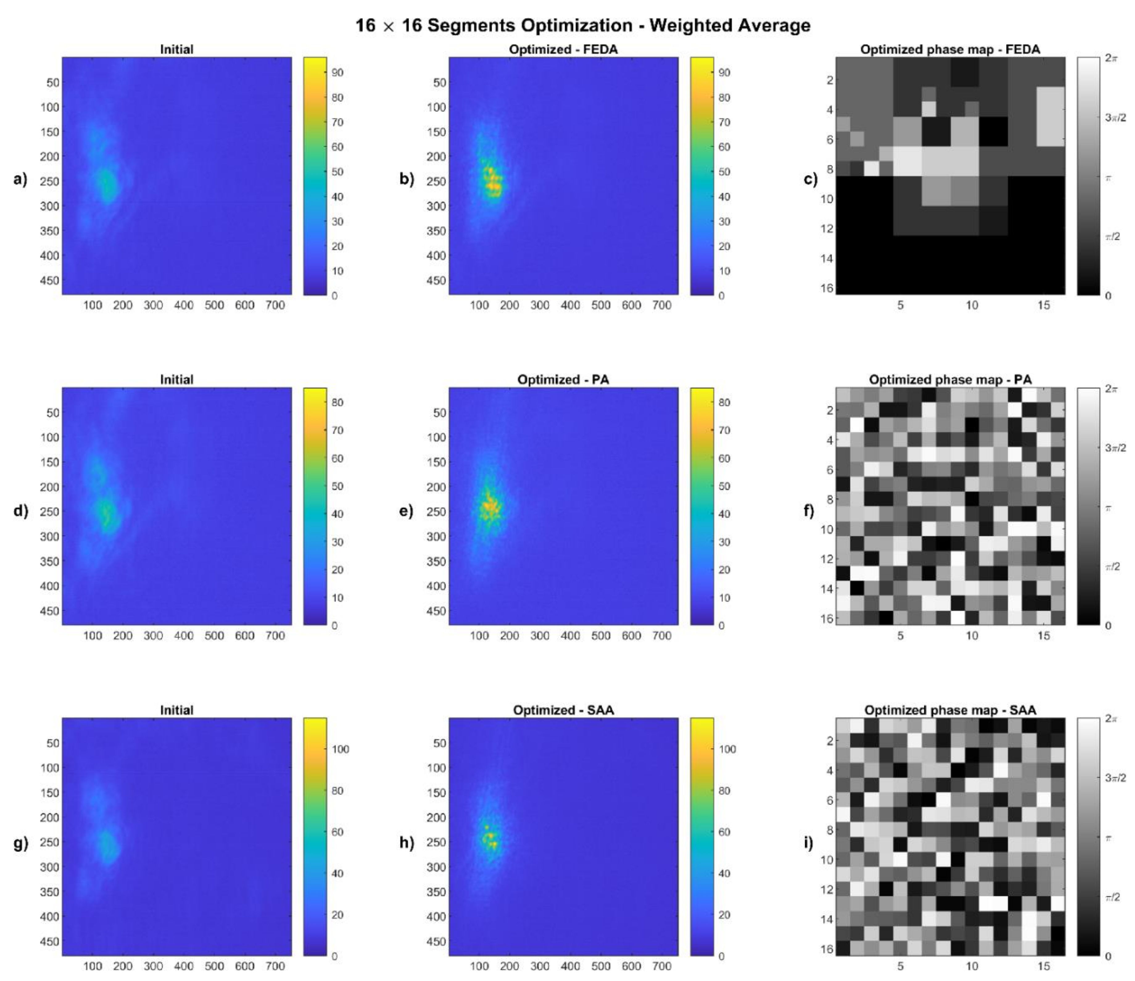
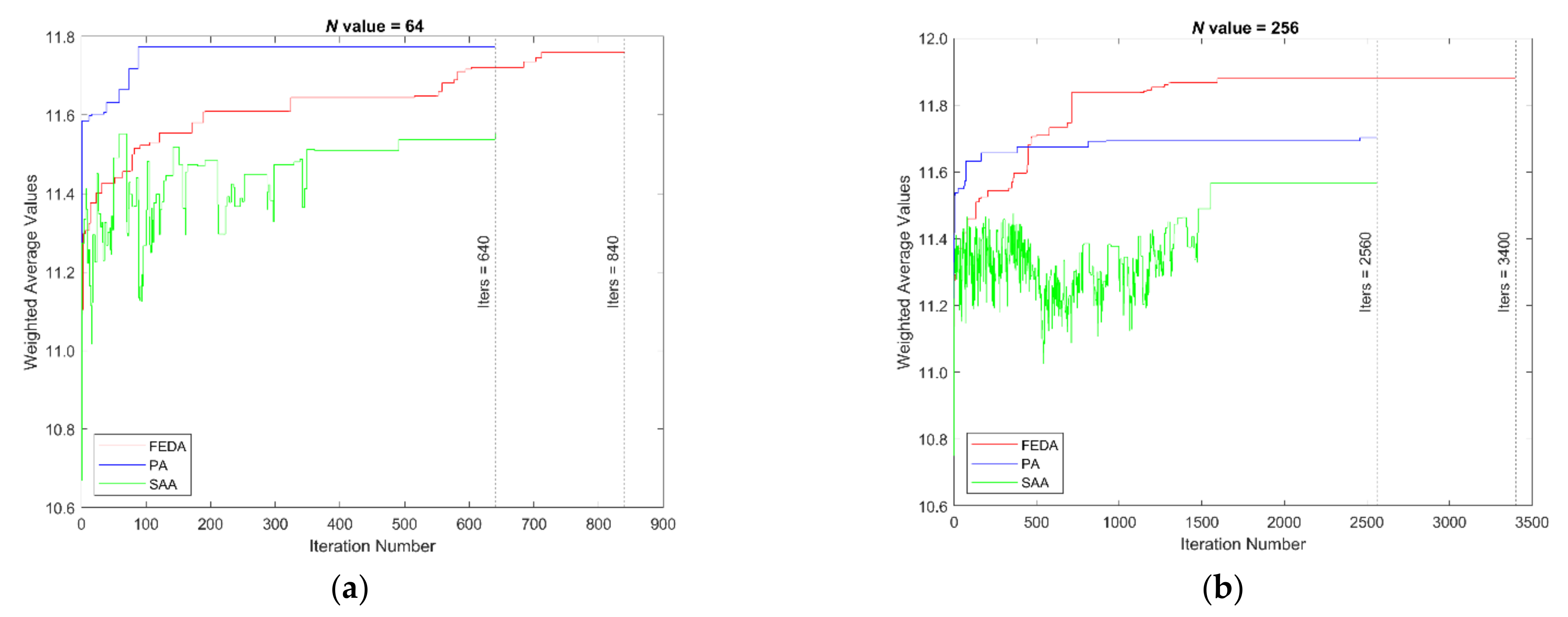
2.4.1. Weighted Average

Based on the calculation of the weighted average of the detector, a phase matrix is applied to the SLM and the optimization is made by maximizing this value while changing the phase matrices. The weighted average is very similar to the calculus of the arithmetic mean with the difference that the contribution given for each data point in a dataset is not the same. Therefore, in this context, this measure relates both the photon intensities read in the pixels of the detector, Icam(x,y), and its distances to a given location in the image. This method allows for assigning different importance to each pixel, referred to as weights, w(x,y), so that the further it is from that selected location, the less contribution it will have to the calculation of the average and to the evolution of the algorithm. In order to calculate the weighted average, first a distance distribution matrix, d(x,y), in pixel units, is calculated in relation to that selected location which represents the spot area (as mentioned above), and the algorithm will evolve by attempting to converge the initial beam’s intensity towards it. Afterwards, the weights distribution is obtained by treating the distances matrix such that the spot location has maximum value (considered as 100) and the most distant pixel(s) from it has a zero value. Having the weights distribution and considering a detector of N × M pixels, the weighted average of an acquired image is calculated as follows:
W a v e r a g e = x = 1 N y = 1 M w x , y · I c a m x , y x = 1 N y = 1 M w x , y .
In this expression, the weights can be normalized, that is, x = 1 N y = 1 M w x , y = 1 with w x , y = w x , y x = 1 N y = 1 M w x , y , simplifying the original formula to:
W a v e r a g e = x = 1 N y = 1 M w x , y · I c a m x , y .
A depiction for the calculation of this value is shown in Figure 4.

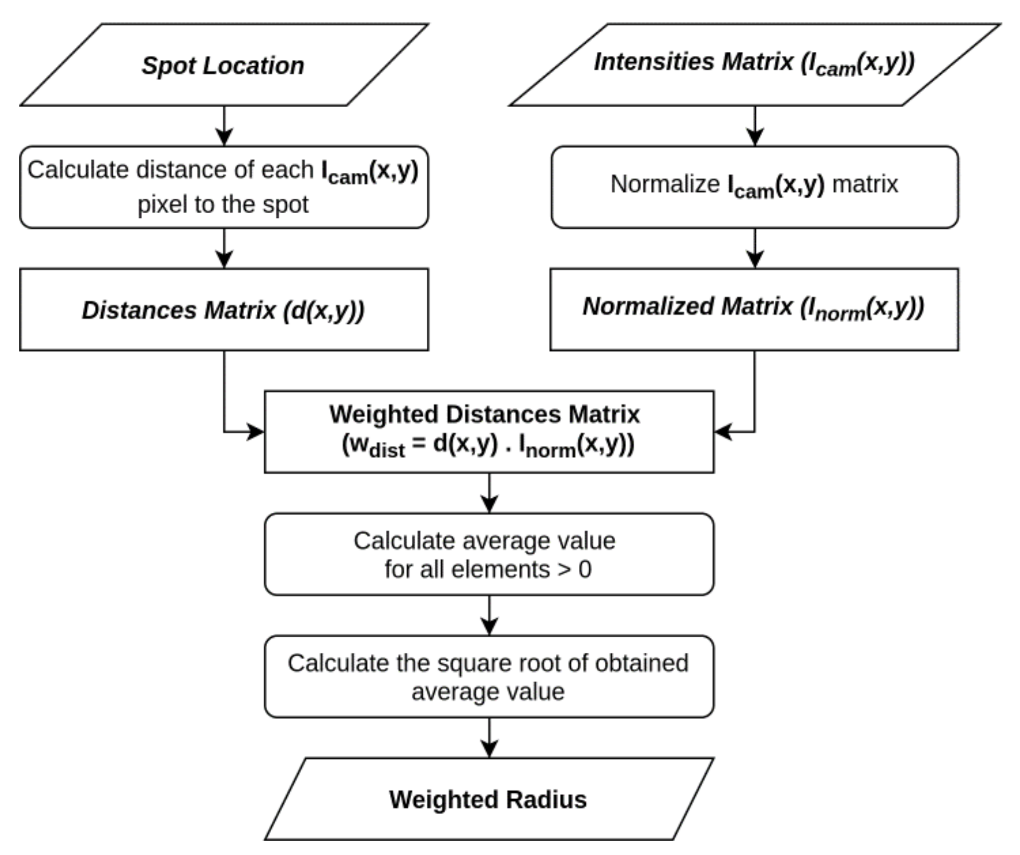
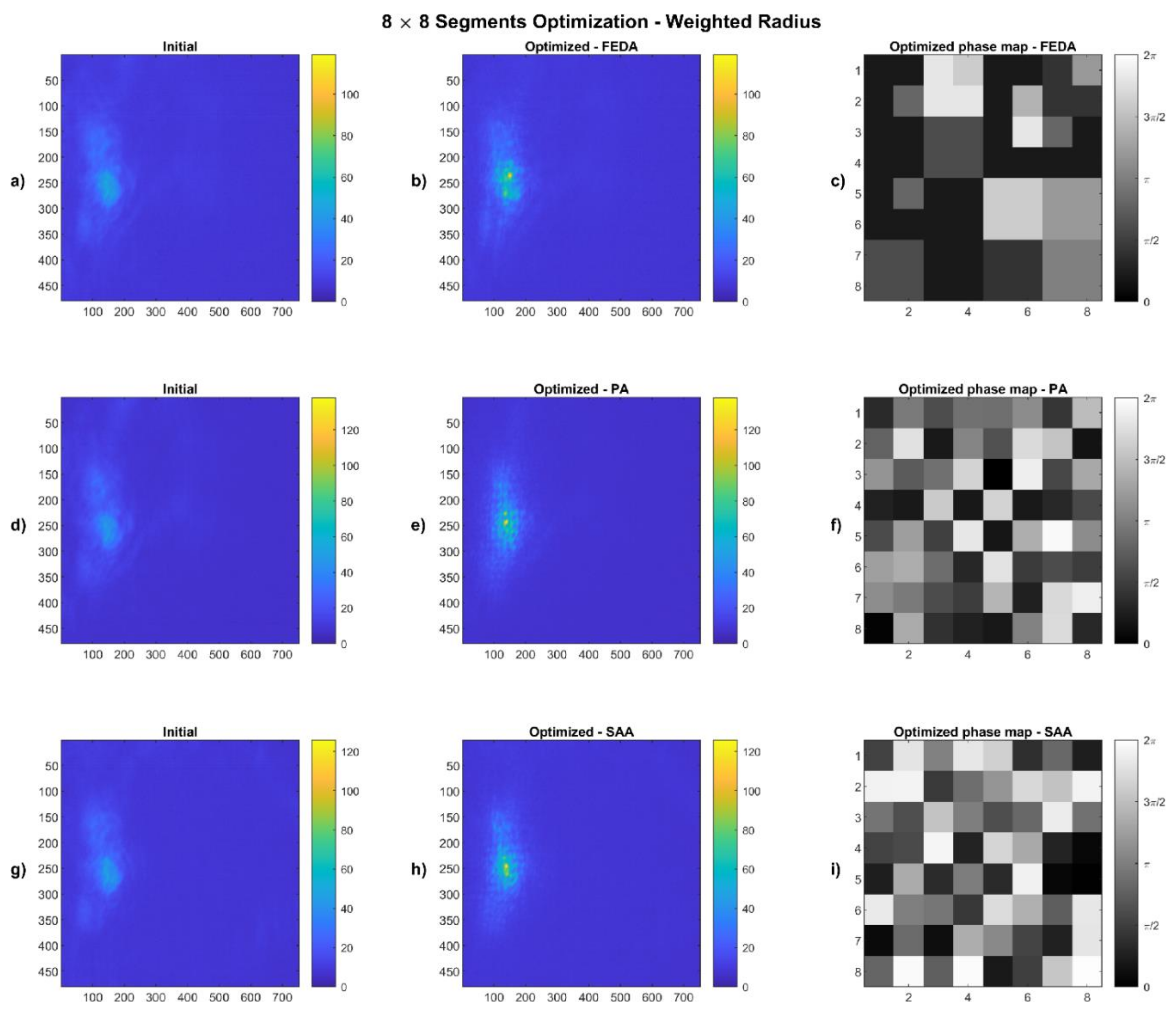
2.4.2. Weighted Radius

The weighted radius is a variant of the weighted average which also takes into consideration the distance of each pixel to a given location. The way that the weighted radius is calculated is by, first, obtaining the distances of every pixel of the camera in relation to that selected location d(x,y). Afterwards, an intensity image is obtained, Icam(x,y), and the relative irradiance matrix is calculated, Inorm(x,y), given by the division of the obtained intensity matrix by the maximum intensity value read. Next, the weighted distance of each pixel is a result of the Hadamard product of the relative irradiance matrix by the previous distances matrix. Finally, the weighted radius is calculated by performing the square root of the average result of the weighted distances, for all the non-zero elements [15]. A scheme for the calculation of this measure is shown in Figure 5.

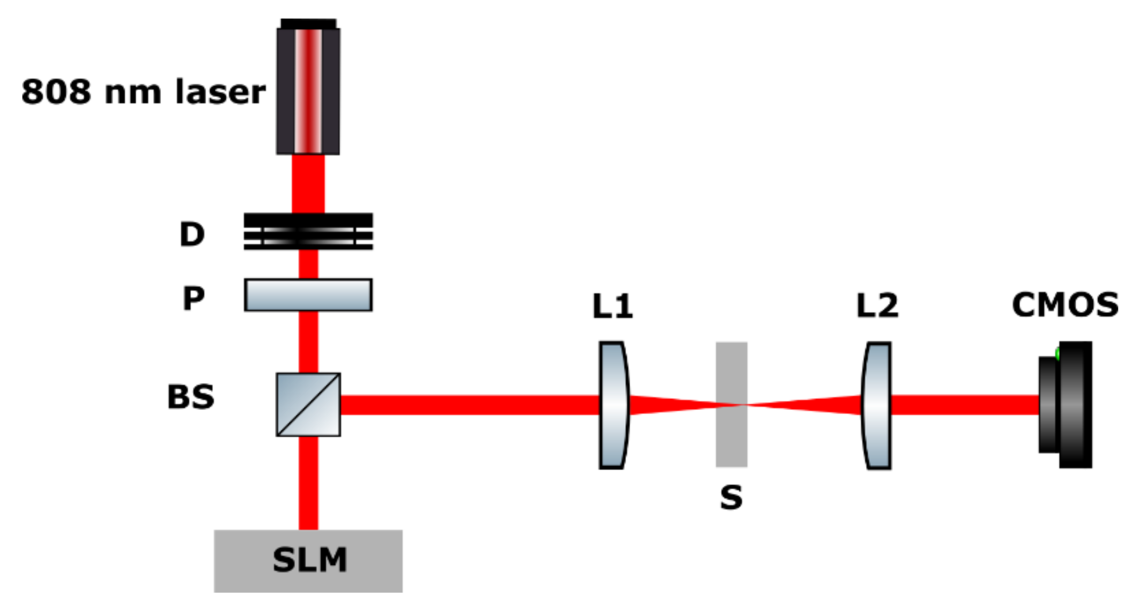
3. Experimental Procedures

The experimental setup is illustrated in Figure 6. A GaAl laser diode produced an 808 nm laser beam in CW (continuous wave) emission. A diaphragm (D) controls the beam diameter and the polarizer (P) assures the spatial filtering of the wavefront, producing linearly polarized incident light aligned parallel to the direction of the liquid crystal molecules of the SLM (Holoeye HEO 1080P Reflective LCOS). This SLM has a resolution of 1920 × 1080 pixels with each pixel having a size of 8 μm × 8 μm. Since the laser beam had a diameter set to 1 mm, only a region of the SLM, with its center aligned with the incident beam, was used for modulating its phase. This working region was set squared with a size of 256 × 256 pixels or 2 mm × 2 mm so that a minimization of the number of non-relevant pixels could be accomplished. A non-polarizer 50/50 beamsplitter (BS) was then used which redirects the reflected laser beam to the optical sample (S) where a focus is produced, at its far end side, by using a converging lens L1 (focal length of 100 mm). The light is then collimated by another converging lens L2 (focal length of 40 mm) and reaches the CMOS camera (AVT Guppy F-036B) that captures its intensities. Due to the adopted configuration and lens positioning, the focal point was represented in the camera as a circular area (i.e., spot) with the same diameter as the incident beam. Then, the captured image is sent to a computer which calculates over it the cost function value and, based on it, changes the configuration of the SLM. The CMOS shutter time was set to a value of 17 ms (~1/60) due to the 60 Hz refresh rate of the SLM in order to average out phase jitter [24]. The data presented and code developed for this study are made available in GitHub https://github.com/jqguerreiro/articleSLM_code.git (accessed on 23 August 2021).
The process of wavefront phase modulation started by first projecting an initial phase matrix onto the working region of the SLM which was considered the zero matrix. This will correspond to having the phase of the incoming beam set to zero and then a value for the cost function (weighted average or weighted radius) is calculated over the acquired intensity image of the detector. Henceforth, the selected algorithm will start its optimization procedure as previously explained. Figure 7 shows a scheme of this wavefront optimization procedure. To be able to compare the performance of every algorithm equally, the laser power was kept constant, as the total number of iterations made (apart from FEDA). The power of the laser was set to 1.5 mW and the total number of iterations for PA and SAA were chosen according to the continuous sequential algorithm (CS) with 10 phase values per cycle. Considering the operation of CS [22], this gives rise to having a total of 640 iterations for the 8 × 8 phase matrix segmentation and 2560 iterations for the 16 × 16 segmentation tests.
Regarding FEDA, the number of iterations made is dependent on the format of the projected phase matrix but also on the number of phase values that are going to be cycled for each segment (n). It was found that, for this algorithm, the expression that gives the total number of iterations for a phase matrix format of 2x × 2x is:
N i t e r s = n i = 1 x 4 i ,   x = 1 ,   2 ,   3 , .
Considering 10 phase values per cycle, an 8 × 8 format results in 840 iterations and a 16 × 16 format results in 3400 iterations.
Regarding PA, the only specific parameter to be set was the total number of iterations, which is related to the total number of perturbations made on the projected phase matrix. Considering SAA, there were several parameters that had to be set, namely the decay factor α, initial temperature T0, and the number of iterations made in a cycle Ncycle. We did not give this algorithm a final temperature since we want it to run a total of 640 or 2560 total iterations, so this was the chosen end criteria. Based on the information in [23], the decay factor and number of iterations made in a cycle were set to α = 0.97, Ncycle = 8 (for 64 segments) and Ncycle = 32 (for 256 segments). With regard to the initial temperature, this was set by taking into consideration Equation (5). By rewriting this equation, we have:
T = E o l d E n e w l n P T
Assuming, due to the nature of the calculus of the weighted average and weighted radius, that these cost functions will produce values with small statistical variation, it was considered a 90% initial probability in accepting a variation of 0.01. By replacing, in Equation (9), E o l d E n e w = 0.01 and P T 0 = 0.9 , we get T 0 = 0.1 for the initial temperature.
An agar-based phantom made up of a mixture of distilled water and milk was used as the test sample, constituting a relatively inexpensive and simple way to simulate a turbid media that resembles the human skin, although there can be several other techniques and materials like gelatin and polyacrylamide gels that successfully produce tissue phantoms [25]. Milk was used as the turbid medium (pasteurized whole milk with a 3.6% lipid content) where the scattering is produced by suspended lipid droplets. The selected human tissue for simulation was the skin of the inner forearm with the optical properties for a wavelength of 808 nm found in [26]. To achieve the required optical properties in producing the tissue phantom, the amount of milk in the mixture had to be set. Regarding the absorption coefficient, both milk and water have similar values that, for this experiment, were considered to be negligible for the working wavelength [27,28], and, since we are interested in suppressing the diffusion effect, this was not taken into account. Therefore, only the scattering amount was set. Regarding the scattering coefficient, for water, this is lesser than its absorption coefficient so only the scattering coefficient of milk was considered [27]. The phantom made for testing was composed of 5% milk with 5 mm of optical length (thickness). This concentration and thickness were chosen for milk with 3.6% fat since it simulates the scattering present in the skin of the inner forearm with an approximate thickness in between 1–2 mm. This approximation was obtained using a metric that was based in the information found in [26,29,30,31]. The following steps explain the phantom’s preparation procedure:
1-
A mixture of 1% agar-agar powder in distilled water was made;
2-
The resulting mixture was heated until its boiling point;
3-
The boiling mixture was left to cool at room temperature;
4-
When the temperature reached a value below 50 °C, the right amount of milk was added to have a 5% milk concentrated mixture;
5-
The resulting mixture was left to cool, for a minimum of 4 h, until use.
In addition to every step, the solution was always being stirred with the exception while being heated in the microwave and in its last cooling process.

4. Results and Discussion

In this section, we present the results for our experiment when choosing the weighted average or the weighted radius as the convergence criteria for all wavefront optimization procedures. We compare the differences when a 8 × 8 or a 16 × 16 phase matrix format is used and, lastly, talk about the differences regarding all algorithms.
In our comparisons, we analyzed measurements like the maximum intensity value achieved and average intensity in the spot area (the representation of the focus point inside the turbid media in the CMOS camera, as explained in Section 2). The improvement over the spot, in percentage, is calculated by:
i m p r o v e m e n t = I o p t . S p o t I 0 S p o t I 0 S p o t × 100 % ,
where I0Spot represents the initial intensity and Iopt.Spot its optimized value.
For the overall convergence of the scattered beam, we take the weighted radius values, calculated without the spot’s intensities, and obtain the improvement based from Equation (10) by replacing the average intensities for the respective weighted radius values. Finally, we also take into consideration the evolution of the cost function values for each algorithm (convergence plots).

4.1. Weighted Average Results

Figure 8 and Figure 9 show the intensity distributions for each algorithm used in the optimization of the weighted average while considering a 64 segment or 256 segment phase matrices, respectively. All left side intensities correspond to the initial phase matrix projected onto the SLM (initial phase matrix), the middle ones relate to the intensities after the optimization, and the right patterns are the optimal phase distributions achieved. All of the approaches seem to have been successful in converging the intensities towards the spot’s center. Regarding FEDA, visually, the optimized results seem to not have many differences when considering either 64 or 256 segments. With PA, more differences can be perceived where an 8 × 8 segmentation led to higher intensity values but a 16 × 16 segmentation appears to have converged more rays towards the center. With SAA, on the contrary, the 8 × 8 optimization seems to have been more successful in recovering the spot’s profile in relation to the 16 × 16 optimization. Table 1 shows the previously referred measurements that allow for better comparing these results. Considering the overall focus improvement, it appears that FEDA achieved better results, whereas PA and SAA allowed for a better focus formation considering a phase matrix of 64 segments. The weighted radius values (outside the spot) consider the overall information of the camera without taking into account the spot region. Therefore, it stands for a measure of the intensities that did not reach the spot but got closer to it. It is seen that the use of more segments results in a higher improvement of this measure, with FEDA achieving, again, the top value.
Figure 10 shows the convergence plots associated with the evolution of the weighted average values in the optimization process. For an 8 × 8 segmentation, it can be seen that for FEDA, an evolution of this parameter is made continuously, with a fast convergence in the first 300 iterations. As for PA, there is an abrupt increase in the first 100 iterations, due to its randomized partition nature, and after which the evolution of the weighted average gets saturated. At this point, the algorithm appears to have been trapped in a local maximum. Finally, with SAA, due to the chosen initial temperature, decay factor and number of iterations made in a cycle, the algorithm accepts worse solutions until around 400 iterations. Although at first sight the SAA seems to be the worst of these three algorithms, in this case, the SAA obtained the largest improvement over the 8 × 8 optimization. It is important to say, though, that the choice of its parameters have no standard method to find [22], which makes the implementation of this method difficult. In addition, different values for these parameters could result in higher improvement values. For a 16 × 16 segmentation, it is seen that FEDA has had the largest improvement, being the evolution of the weighted average saturated at about 2000 iterations. The explanation for this can be seen by its optimal phase matrix where the bottom half has no smaller segment changes, so the phase cycling over all smaller segments in this half had no positive influence over the cost function. Regarding PA, similarly to the previous case, there was an abrupt increase in the first 1000 iterations after which the optimization process did not lead to major intensity changes. With SAA, the algorithm accepted worse solutions until around 1500 iterations. After that, a large increase of the cost function was observed and, at around 2000 iterations, it seems that this approach reached its saturation point.
In summary, SAA and PA have shown greater improvement by 64 segments (improvement of 50%), whereas FEDA overcomes these two algorithms when using 256 segments (improvement of 51%). Regarding consistency, FEDA has proven to be the best algorithm having high improvement values considering both 64 and 256 segments.

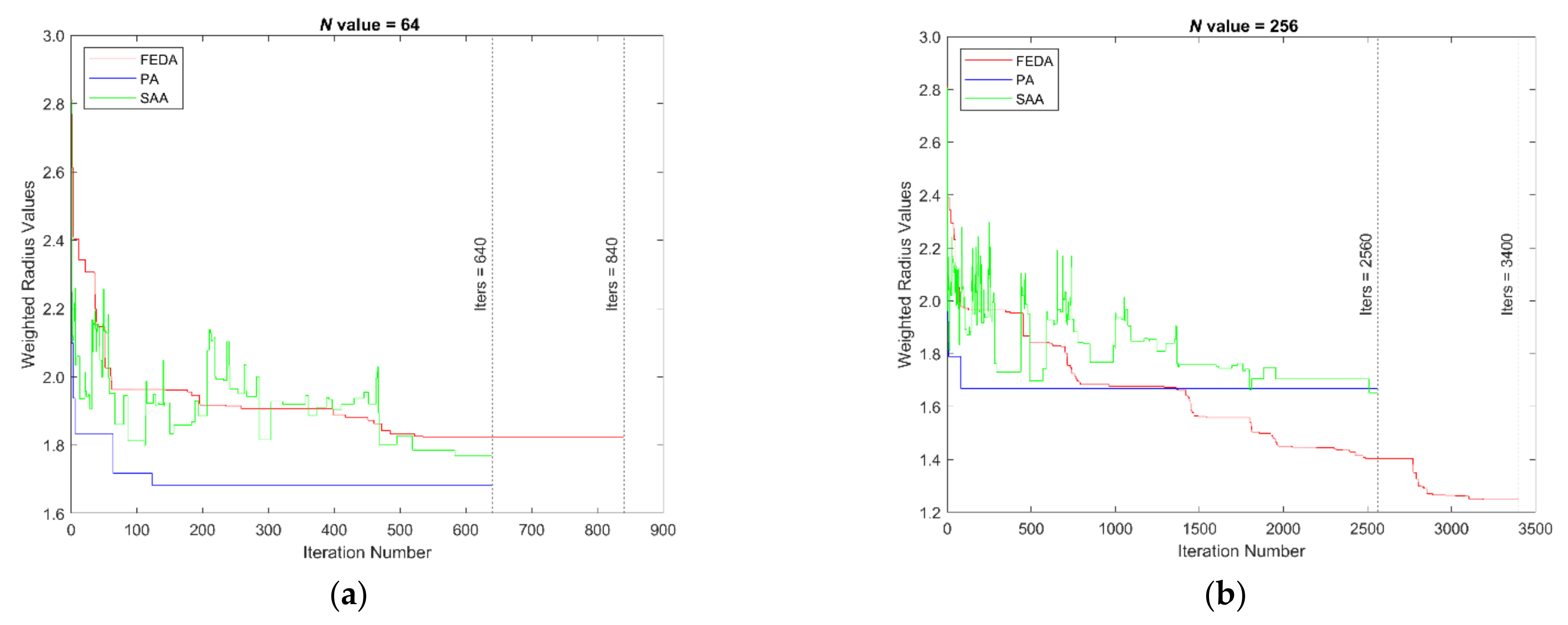
4.2. Weighted Radius Results

Figure 11 and Figure 12 show the intensity distributions for each algorithm used in the optimization of the weighted radius. One can see right away that the optimization, in all cases, resulted in a quite different scenario than the previous results. It is seen that a very intense point inside the spot was now formed. For every algorithm, the use of 256 segments results in a sharper focal point in comparison with 64 segments. By looking at the information of Table 2, it is concluded that, with FEDA, by increasing the number of segments, the spot improvement increased to a top value of 46%. With PA and SAA, on the contrary, the increase in number of segments led to a decrease of improvement, the 8×8 segmentation being the better solution. Regarding the intensities outside the spot, both FEDA and SAA showed to be better in converging the ray beams towards the spot.
Figure 13 shows the convergence plots concerning the evolution of the weighted radius. Similarly to the weighted average case, the PA rapidly achieves its saturation point in the 100th iteration mark (for 64 segments) and in the 1000th iteration (for 256 segments). For 8 × 8 segmentation, it is seen that FEDA has a fast convergence in the first 200 iterations, after which the evolution of this parameter slows down due to less significance of the phase changes of the smallest segments of the bottom half of the phase distribution. With SAA, the specific parameters might not have been finely tuned since it accepts worse solutions until the 500th iteration mark, near its end. Nevertheless, it resulted in a higher improvement than FEDA’s. For the 16 × 16 segmentation, FEDA has a continuous evolution role, whereas SAA still has a rather large range of iterations where it accepts worse solutions. For this latter case, both SAA and PA seem to achieve similar improvement values.

4.3. Final Assessment

Lastly, we would like to provide an assessment on the differences stated for every algorithm tested, summarized on Table 3. On the weighted average and weighted radius methods, we can assign to the PA the strengths of having the fastest increase at the beginning, after which the algorithm does not go through much evolution. A negative of this algorithm is that most of the iterations have not seen great changes or a continuous evolution of the algorithm since it has been stuck in its local minimum/maximum. This occurs due to the algorithm’s nature where the optimized result will be very dependent on the first best accepted solution. As for SAA, its behavior of accepting worse solutions bypasses the limitation of PA in getting trapped in a local minimum/maximum, where a continuous evolution attempt is made. However, SAA has high sensitivity to the change of its specific parameters, which, despite making it very adaptable to situations, results in it being hard to work with (and can explain why the 8 × 8 segmentation resulted in better improvements than the 16 × 16 segmentation). These parameters have to be chosen or tuned, which requires some insight on the cost function evolution behavior. Finally, FEDA produces the best results overall given its nature that allows for checking each individual segment the phase that results in a best cost function value. As for the only considered disadvantage, FEDA requires more iterations in achieving its optimized result, which, in reality, will result in a longer process.

5. Conclusions

We have performed phase modulation of the incident wavefront of an 808 nm laser in an iterative approach for compensation of the scattering effects of a turbid sample mimicking 1–2 mm of human skin. The use of milk in reproducing the scattering effects of biological tissue was done, constituting an inexpensive way in building a tissue phantom. Higher irradiance values over the focal spot were successfully achieved in testing three different optimization algorithms over two different evolution criteria. The weighted average proved to be a better choice over the weighted radius in achieving the desired goal. Both SAA and PA showed similar improvements with the difference that PA has a very fast convergence in the initial iterations and does not require many input parameters, that in SAA are not easy to set. PA showed a final top improvement of 49%. FEDA also proved to be a great candidate, especially with 256 segments where its top improvement was 51%. Despite larger iterations being required, it could be of interest to combine both FEDA and PA such that, in the initial iterations, PA would be executed and after which, for the optimization of the smallest segments, FEDA would take on the responsibility. This could significantly reduce FEDA’s total iterations and would lead to having good improvement values in less time. In future applications of the method, the increase irradiance will require attention to safety issues. In particular, the maximum permissible exposure of the laser light threshold on the tissue must be guaranteed from the start to the end of the iterative process. This value depends on the radiation wavelength and on the time of exposure and can be defined in terms of radiation dose, which depends on the irradiation time, the power of the radiation used, and the irradiated area. The International Commission on Non-Ionizing Radiation Protection, ICNIRP, published in 2013 [32] the guidelines for the exposure limits to laser radiation depending on the wavelength and time of exposure. When using 808 nm wavelength laser radiation for a duration from 10 s to 30 ks, the exposure limit for the skin is 0.33 W/ cm 2 (in our tests, we had 0.048 W/ cm 2 ) and, if the phase shaping process allows a reduction in, for example, 27% of the beam radius, the irradiance increases by almost 88%. Nevertheless, as also stated by the ICNIRP [33], the exposure limit can be exceeded for diagnostic and therapeutic purposes when the intended benefits of the procedure overcome the potential side effects. Future work will also include adapting the experimental setup to use backscattering radiation instead of transmitted radiation to obtain feedback information for the algorithms, and thus make the technique applicable in the medical environment.

Author Contributions

Conceptualization, J.M.P.C. and P.V.; methodology, J.G.; software, J.G.; validation, J.G.; formal analysis, J.M.P.C., J.G., and P.V.; investigation, J.G. and J.M.P.C.; writing—original draft preparation, J.G.; writing—review and editing, J.M.P.C., J.G., and P.V. All authors have read and agreed to the published version of the manuscript.

Funding

This research was funded by Fundação para a Ciência e Tecnologia (FCT), Grant No. UIDB/00645/2020.

Institutional Review Board Statement

Not applicable.

Informed Consent Statement

Not applicable.

Data Availability Statement

The data presented and code developed for this study are made available in GitHub https://github.com/jqguerreiro/articleSLM_code.git (accessed on 23 August 2021).

Acknowledgments

The authors would like to thank and show their appreciation to Lin Pang for the insight provided on this research topic.

Conflicts of Interest

The authors declare no conflict of interest.

References

  1. Coelho, J.M.P.; Vilhena, H.; Rebordão, J.M. Finite element model for the simulation of laser activated micro- and nano-scale drug delivery systems. In Proceedings of the Third International Conference on Applications of Optics and Photonics, Faro, Portugal, 8–12 May 2017; Volume 10453, p. 104531Y. [Google Scholar] [CrossRef]
  2. Daraee, H.; Eatemadi, A.; Abbasi, E.; Aval, S.F.; Kouhi, M.; Akbarzadeh, A. Application of gold nanoparticles in biomedical and drug delivery. Artif. Cells Nanomed. Biotechnol. 2016, 44, 410–422. [Google Scholar] [CrossRef]
  3. Mirza, F.N.; Khatri, K.A. The use of lasers in the treatment of skin cancer: A review. J. Cosmet. Laser Ther. 2017, 19, 451–458. [Google Scholar] [CrossRef]
  4. Jain, S.M.; Pandey, K.; Lahoti, A.; Rao, P.K. Evaluation of skin and subcutaneous tissue thickness at insulin injection sites in Indian, insulin naïve, type-2 diabetic adult population. Indian J. Endocrinol. Metab. 2013, 17, 864–870. [Google Scholar] [CrossRef]
  5. Schena, E.; Saccomandi, P.; Fong, Y. Laser ablation for cancer: Past, present and future. J. Funct. Biomater. 2017, 8, 19. [Google Scholar] [CrossRef] [Green Version]
  6. Singh, P.; Pandit, S.; Mokkapati, V.R.S.S.; Garg, A.; Ravikumar, V.; Mijakovic, I. Gold nanoparticles in diagnostics and therapeutics for human cancer. Int. J. Mol. Sci. 2018, 19, 1979. [Google Scholar] [CrossRef] [PubMed]
  7. Lopes, J.; Coelho, J.M.P.; Vieira, P.M.C.; Viana, A.S.; Gaspar, M.M.; Reis, C. Preliminary assays towards melanoma cells using phototherapy with gold-based nanomaterials. Nanomaterials 2020, 10, 1536. [Google Scholar] [CrossRef]
  8. Lopes, A.; Gomes, R.; Castiñeras, M.; Coelho, J.M.P.; Santos, J.P.; Vieira, P. Probing deep tissues with laser-induced thermotherapy using near-infrared light. Lasers Med. Sci. 2020, 35, 43–49. [Google Scholar] [CrossRef] [PubMed]
  9. Amendola, V.; Pilot, R.; Frasconi, M.; Maragò, O.M.; Iatì, M.A. Surface plasmon resonance in gold nanoparticles: A review. J. Phys. Condens. Matter 2017, 29, 203002. [Google Scholar] [CrossRef] [PubMed]
  10. Weissleder, R. A clearer vision for in vivo imaging: Progress continues in the development of smaller, more penetrable probes for biological imaging. Nat. Biotechnol. 2001, 19, 316–317. [Google Scholar] [CrossRef] [PubMed]
  11. Gomes, R.; Coelho, J.M.P.; Gabriel, A.; Vieira, P.; Oliveira Silva, C.; Reis, C. Wavefront shaping using a deformable mirror for focusing inside optical tissue phantoms. In Proceedings of the Second International Conference on Applications of Optics and Photonics, Aveiro, Portugal, 26–30 May 2014; Volume 9286, p. 92863Z. [Google Scholar] [CrossRef]
  12. Yu, H.; Park, J.; Lee, K.; Yoon, J.; Kim, K.; Lee, S.; Park, Y. Recent advances in wavefront shaping techniques for biomedical applications. Curr. Appl. Phys. 2015, 15, 632–641. [Google Scholar] [CrossRef] [Green Version]
  13. Wei, Q.; Huang, L.; Zentgraf, T.; Wang, Y. Optical wavefront shaping based on functional metasurfaces. Nanophotonics 2020, 9, 987–1002. [Google Scholar] [CrossRef]
  14. Tay, J.W.; Lai, P.; Suzuki, Y.; Wang, L.V. Ultrasonically encoded wavefront shaping for focusing into random media. Sci. Rep. 2014, 4, 1–5. [Google Scholar] [CrossRef] [Green Version]
  15. Gomes, R.; Vieira, P.; Coelho, J.M.P. Optical simulation of laser beam phase-shaping focusing optimization in biological tissues. In Proceedings of the 8th Ibero American Optics Meeting/11th Latin American Meeting on Optics, Lasers, and Applications, Porto, Portugal, 22–26 July 2013; Volume 8785, p. 8785DE. [Google Scholar] [CrossRef]
  16. Kanngiesser, J.; Roth, B. Wavefront shaping concepts for application in optical coherence tomography—A review. Sensors 2020, 20, 7044. [Google Scholar] [CrossRef]
  17. Fayyaz, Z.; Mohammadian, N.; Salimi, F.; Fatima, A.; Tabar, M.R.R.; Avanaki, M.R.N. Simulated annealing optimization in wavefront shaping controlled transmission. Appl. Opt. 2018, 57, 6233. [Google Scholar] [CrossRef]
  18. Tseng, S.H.; Yang, C. 2-D PSTD Simulation of optical phase conjugation for turbidity suppression. Opt. Express 2007, 15, 16005. [Google Scholar] [CrossRef] [PubMed] [Green Version]
  19. Fayyaz, Z.; Salimi, F.; Mohammadian, N.; Fatima, A.; Rahimi Tabar, M.R.; Avanaki, M.R.N. Wavefront shaping using simulated annealing algorithm for focusing light through turbid media. In Proceedings of the Photons Plus Ultrasound: Imaging and Sensing, San Francisco, CA, USA, 28 January–1 February 2018; Volume 10494, p. 104946M. [Google Scholar] [CrossRef]
  20. Fayyaz, Z.; Mohammadian, N.; Avanaki, M.R.N. Comparative assessment of five algorithms to control an SLM for focusing coherent light through scattering media. In Proceedings of thePhotons Plus Ultrasound: Imaging and Sensing, San Francisco, CA, USA, 28 January–1 February 2018; Volume 10494, p. 104946I. [Google Scholar] [CrossRef]
  21. Fang, L.; Zhang, X.; Zuo, H.; Pang, L. Focusing light through random scattering media by four-element division algorithm. Opt. Commun. 2018, 407, 301–310. [Google Scholar] [CrossRef]
  22. Vellekoop, I.M.; Mosk, A.P. Phase control algorithms for focusing light through turbid media. Opt. Commun. 2008, 281, 3071–3080. [Google Scholar] [CrossRef] [Green Version]
  23. Fang, L.; Zuo, H.; Yang, Z.; Zhang, X.; Pang, L. Focusing light through random scattering media by simulated annealing algorithm. J. Appl. Phys. 2018, 124, 083104. [Google Scholar] [CrossRef]
  24. Vellekoop, I.M.; Aegerter, C.M. Focusing light through living tissue. In Proceedings of the Optical Coherence Tomography and Coherence Domain Optical Methods in Biomedicine XIV, San Francisco, CA, USA, 25–27 January 2010; Volume 7554, p. 755430. [Google Scholar] [CrossRef] [Green Version]
  25. Ntombela, L.; Adeleye, B.; Chetty, N. Low-cost fabrication of optical tissue phantoms for use in biomedical imaging. Heliyon 2020, 6, e03602. [Google Scholar] [CrossRef]
  26. Kono, T.; Yamada, J. In Vivo measurement of optical properties of human skin for 450–800 nm and 950–1600 nm wavelengths. Int. J. Thermophys. 2019, 40, 1–14. [Google Scholar] [CrossRef] [Green Version]
  27. Stocker, S.; Foschum, F.; Krauter, P.; Bergmann, F.; Hohmann, A.; Happ, C.S.; Kienle, A. Broadband optical properties of milk. Appl. Spectrosc. 2017, 71, 951–962. [Google Scholar] [CrossRef] [PubMed]
  28. Hale, G.M.; Querry, M.R. Optical constants of water in the 200-nm to 200-μm wavelength region. Appl. Opt. 1973, 12, 555. [Google Scholar] [CrossRef] [PubMed]
  29. Jacques, S.L. Optical properties of biological tissues: A review. Phys. Med. Biol. 2013, 58, R37–R61. [Google Scholar] [CrossRef] [PubMed]
  30. Ortega-Quijano, N.; Fanjul-Vélez, F.; Salas-García, I.; Arce-Diego, J.L. Optical characterization of lipid-based tissue phantoms. In Proceedings of the 21st International Conference Radioelektronika, Brno, Czech Republic, 19–20 April 2011; pp. 107–110. [Google Scholar] [CrossRef]
  31. Aernouts, B.; Van Beers, R.; Watté, R.; Huybrechts, T.; Lammertyn, J.; Saeys, W. Visible and near-infrared bulk optical properties of raw milk. J. Dairy Sci. 2015, 98, 6727–6738. [Google Scholar] [CrossRef] [PubMed] [Green Version]
  32. Ziegelberger, G. ICNIRP guidelines on limits of exposure to laser radiation of wavelengths between 180 nm and 1000 µm. Health Phys. 2013, 105, 271–295. [Google Scholar]
  33. Ziegelberger, G.; van Rongen, E.; Croft, R.; Feychting, M.; Green, A.C.; Hirata, A.; d’Inzeo, G.; Marino, C.; Miller, S.; Oftedal, G.; et al. Principles for non-ionizing radiation protection. Health Phys. 2020, 118, 477–482. [Google Scholar]
Figure 1. FEDA principle (based on [13]). This scheme shows phase optimization for 4 × 4 format. (ad) Phase modulation of 4 segments of the initial phase matrix in the 2 × 2 format. (eh) Division of the first segment into 4 equal sized segments and phase modulation for these smaller segments while having the optimized phase values set. (i) The procedure made in (eh) is repeated for the second segment of the 2 × 2 initial phase format. (j) The remaining two segments follow the same steps until an optimized 4 × 4 phase matrix is achieved.
Photonics 08 00355 g001
Figure 2. PA principle: (ac) random selection of half the segments and phase setting with random values in between 0–2 π ; (d) final optimized phase map. This scheme shows phase optimization for 4 × 4 format (based on [14]).
Photonics 08 00355 g002
Figure 3. SAA principle’s scheme.
Photonics 08 00355 g003
Figure 4. Weighted Average diagram based from Equation (6) that requires both the spot location in the camera, as pixel coordinates, and the captured intensities as inputs. For the calculation of the value of the weighted average, the weights distribution and captured intensity are required. The weights distribution is going to be of the size of the captured intensities, where first the distance of each pixel of the camera to the spot’s location in the image is calculated. Then, this result is updated in having values in the range of 0–100 where 0 corresponds to the pixels of the spot and 100 the most distant pixel(s) from it—weights distribution. Finally, by having the required variables for directly calculating the weighted average from Equation (6), the same is obtained.
Photonics 08 00355 g004
Figure 5. Weighted Radius diagram that takes both the spot location in the camera, as pixel coordinates, and the captured intensities as inputs. For the calculation of the value of the weighted radius, the normalized captured intensities and distances of each pixel of the camera to the spot are required. The distances matrix is of the same size of the captured intensities, where similarly to the case of the weighted average, each value will correspond to the distance of that pixel to the spot’s location in the image. Next, the normalized intensities matrix is obtained by dividing each pixel’s intensity value by the maximum pixel intensity read. Then, the weighted radius can be calculated by obtaining the square root of the selective average (discarding null values) of the Hadamard product between the distances matrix and normalized intensity matrix.
Photonics 08 00355 g005
Figure 6. Schematic of the experimental setup. Letters represent: D: Diaphragm; P: Polarizer; BS: Beamsplitter; L1, L2: Plano-convex lens; S: Sample.
Photonics 08 00355 g006
Figure 7. Feedback-based wavefront shaping diagram while using a SLM. The dark squared shape is representing the initial phase matrix applied to the SLM and the one below is representing the disturbed phase matrix, where several segments change its phase value.
Photonics 08 00355 g007
Figure 8. Results for the 8 × 8 segmentation of the phase map with the weighted average being the cost function. (a,b), (d,e), (g,h) stand for the initial and optimized intensity distributions captured by the CMOS when running FEDA, PA, and SAA algorithms, respectively. All initial’s intensity distributions were captured before running each algorithm and after setting the phase of the incident beam to zero. For the intensity distributions, the grid values correspond to pixel units of the CMOS and the colorbar/intensity range can have values in between 0–255. (c,f,i) are the achieved optimal phase maps/matrices projected in the SLM after running FEDA, PA, and SAA, respectively. For the phase maps, its values range from 0 (black) to 2 π (white) with 10 values in between this range.
Photonics 08 00355 g008
Figure 9. Results for the 16 × 16 segmentation of the phase map with the weighted average being the cost function. (a,b), (d,e), (g,h) stand for the initial and optimized intensity distributions captured by the CMOS when running FEDA, PA, and SAA algorithms, respectively. All initial’s intensity distributions were captured before running each algorithm and after setting the phase of the incident beam to zero. For the intensity distributions, the grid values correspond to pixel units of the CMOS and the colorbar/intensity range can have values in between 0–255. (c,f,i) are the achieved optimal phase maps/matrices projected in the SLM after running FEDA, PA, and SAA, respectively. For the phase maps, its values range from 0 (black) to 2 π (white) with 10 values in between this range.
Photonics 08 00355 g009
Figure 10. Convergence plots for the weighted average: (a) optimization with 8 × 8 segmentation; (b) optimization with 16 × 16 segmentation.
Photonics 08 00355 g010
Figure 11. Results for the 8 × 8 segmentation of the phase map with the weighted radius being the cost function. (a,b), (d,e), (g,h) stand for the initial and optimized intensity distributions captured by the CMOS when running FEDA, PA, and SAA algorithms, respectively. All initial’s intensity distributions were captured before running each algorithm and after setting the phase of the incident beam to zero. For the intensity distributions, the grid values correspond to pixel units of the CMOS, and the colorbar/intensity range can have values in between 0–255. (c,f,i) are the achieved optimal phase maps/matrices projected in the SLM after running FEDA, PA, and SAA, respectively. For the phase maps, its values range from 0 (black) to 2 π (white) with 10 values in between this range.
Photonics 08 00355 g011
Figure 12. Results for the 16 × 16 segmentation of the phase map with the weighted radius being the cost function. (a,b), (d,e), (g,h) stand for the initial and optimized intensity distributions captured by the CMOS when running FEDA, PA, and SAA algorithms, respectively. All initial’s intensity distributions were captured before running each algorithm and after setting the phase of the incident beam to zero. For the intensity distributions, the grid values correspond to pixel units of the CMOS and the colorbar/intensity range can have values in between 0–255. (c,f,i) are the achieved optimal phase maps/matrices projected in the SLM after running FEDA, PA, and SAA, respectively. For the phase maps, its values range from 0 (black) to 2 π (white) with 10 values in between this range.
Photonics 08 00355 g012
Figure 13. Convergence plots for the weighted radius: (a) optimization with 8 × 8 segmentation; (b) optimization with 16 × 16 segmentation.
Photonics 08 00355 g013
Table 1. Measurements for the weighted average optimization.
AlgorithmSegmentation Max. I Value (0–255)Av. Intensity in SpotImprovementWeighted Radius (Outside the Spot)Improvement
FEDA8 × 8Initial5230.7545%3.4317%
Optimized9444.382.84
16 × 16Initial5230.8351%3.4826%
Optimized9646.572.59
PA8 × 8Initial5230.9249%3.2617%
Optimized10845.932.72
16 × 16Initial5331.0434%3.3119%
Optimized8541.472.70
SAA8 × 8Initial5029.9050%3.4721%
Optimized10644.522.73
16 × 16Initial5129.9339%3.4424%
Optimized11541.602.61
Table 2. Measurements for the weighted radius optimization.
AlgorithmSegmentation Max. I Value (0–255)Av. Intensity in SpotImprovementWeighted Radius (Outside the Spot)Improvement
FEDA8 × 8Initial5130.6430%3.5318%
Optimized11939.902.90
16 × 16Initial5130.6446%3.5325%
Optimized25344.732.65
PA8 × 8Initial5230.7541%3.2715%
Optimized13843.342.77
16 × 16Initial5230.6133%3.4118%
Optimized14240.612.78
SAA8 × 8Initial5129.7138%3.7027%
Optimized12641.012.70
16 × 16Initial5129.7234%3.5824%
Optimized14539.842.71
Table 3. Pluses and minuses of using each optimization algorithm.
Algorithm+
FEDA
  • Overall produces the best results
  • Has a continuous evolution
  • Requires more iterations/Takes more time
PA
  • Has a very fast increase at start
  • Easy to work with
  • Gets stuck in a local minimum/maximum
SAA
  • Does not get stuck in a local minimum/maximum
  • Adaptable by correctly choosing its specific input parameters
  • Specific parameters have to be tuned. Requires some a priori knowledge on the behavior of the cost function values
  • Harder to work with
Publisher’s Note: MDPI stays neutral with regard to jurisdictional claims in published maps and institutional affiliations.

