Abstract
Coherent beam combining (CBC) with closely arranged centrosymmetric arrays is a promising way to obtain a high-brightness laser. An essential task in CBC is to actively control the piston phases of the input beams, maintaining the correct phasing to maximize the combination efficiency. By applying the neural network, the nonlinear mapping relationship between the far-field image and the piston phase could be established, so that the piston phase can be corrected quickly with one step, which caused widespread concern. However, there exists a piston-type phase ambiguity problem in the CBC system with centrosymmetric arrays, which means that multiple different piston phases may generate the same far-field image. This will prevent the far-field image from correctly reflecting the phase information, which will result in a performance degradation of the image-based intelligent algorithms. In this paper, we make a theoretical analysis of phase ambiguity. A method to solve phase ambiguity is proposed, which requires no additional optical devices. We designed simulations to verify our conclusions and methods. We believe that our work solves the phase ambiguity problem in theory and is conducive to improving the performance of image-based algorithms.
1. Introduction
High-power lasers are widely applied in many fields, including Lidar systems, Space Communication, Laser Medicine, Material Processing, and so on [1,2,3,4,5,6]. Therefore, obtaining high-power lasers has important practical value. The laser output with high power and high beam quality can be obtained in the far-field by combining multiple low-power laser beams to keep the phase difference between sub-beams as an integral multiple of 2π [1,2,7,8,9,10]. Chang et al. firstly demonstrated the coherent beam combining (CBC) of more than 100 beams [11]. Civan Laser reported a CBC system with an output laser power of more than 10 kW [12]. The results show that the co-phase output in the CBC system is a promising method to obtain a high-power output.
The core challenge of achieving a co-phase output is to correct and lock the piston phase quickly between each sub-beam [13,14,15,16,17,18,19]. In the past, a series of phase-locking methods have been proposed, including the dithering technique [20,21,22], interference measurement [23,24], and stochastic parallel gradient descent (SPGD) [25,26]. The dithering technique and the interference measurement method need to add new devices to the CBC system. The optimization algorithms cost a number of iterative steps before reaching convergence, which limits their application in practice. With the development of deep learning, various intelligent algorithms are introduced into CBC [27,28,29,30]. Researchers expect to use neural network (NN) models to establish the mapping between the far-field and the piston phase, and compensate the current piston phase with a prediction to realize the co-phase, which helps to reduce iterative steps. In 2019, Hou et al. predicted the rough value of the piston phase according to the far-field image at the defocus plane with a convolutional neural network (CNN), and then applied SPGD based on the prediction, so as to increase the convergence speed [27]. In 2020, Liu et al. employed CNN to measure the beam-pointing and piston phase of sub-beams from the far-field image in a two-beam coherent beam combining system [28]. These studies indicate that the introduction of image information can effectively improve the convergence-performance of the algorithm.
Although the algorithm based on deep learning shows a competitive performance, its interpretability has yet to be discussed. Researchers want to know whether the model learned to “infer” or “remember”. The problem is whether the piston phase can be directly predicted from the far-field with one step in theory. We notice that the model will not converge in some cases. For example, researchers find that a piston-type phase ambiguity exists in centrosymmetric arrays [31,32], which means that different piston phases may generate the same far-field image. In this case, the far-field image cannot provide sufficient information of the current piston phase, interfering with the model’s learning (we will show this in Section 4). Due to such phenomena, predictions of NN are reliable only when all the causes of phase ambiguity have been solved. Our main work is to analyze the mechanism of phase ambiguity and find its solution, which is helpful to supplement the interpretability of deep-learning-based algorithms as well. After that, the introduced image information will accurately reflect the piston phase, which is helpful for a high-speed and accurate prediction.
2. Principle
2.1. Discussion on Piston-Type Phase Ambiguity
The diagram of the CBC system is shown in Figure 1. We divide the laser into N elements by a fiber splitter. (N is the number of sub-apertures.) The power amplifier (PA) is employed to amplify the power of each sub-beam. After that, the piston phases of the amplified sub-beams are controlled by the phase modulator (PM). The output sub-beams are focused by a transform lens, and then the focused sub-beams are split by a beam-splitter (BS) into two beams. One beam is sent to a 10× micro-objective (MO) and detected by a CCD camera to obtain the far-field image for phase-locking. Another beam is transformed to the target face for practical application.
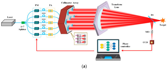
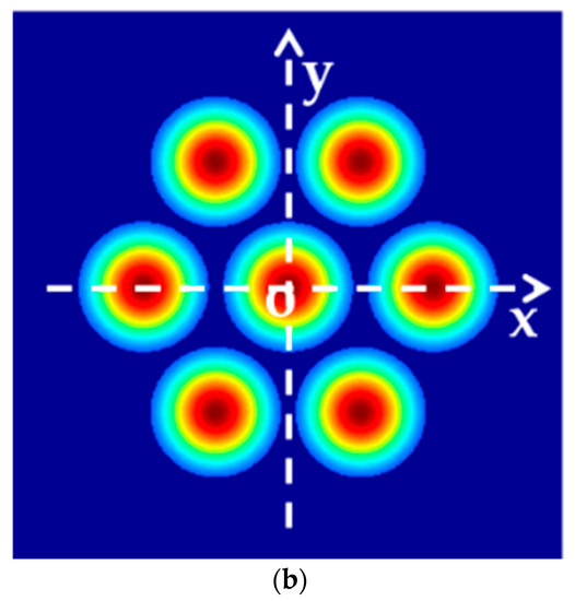
Figure 1.
(a) The structure of the N-elements CBC system (N = 7 in this diagram); (b) Schematic diagram of the emissive plane coordinate system.
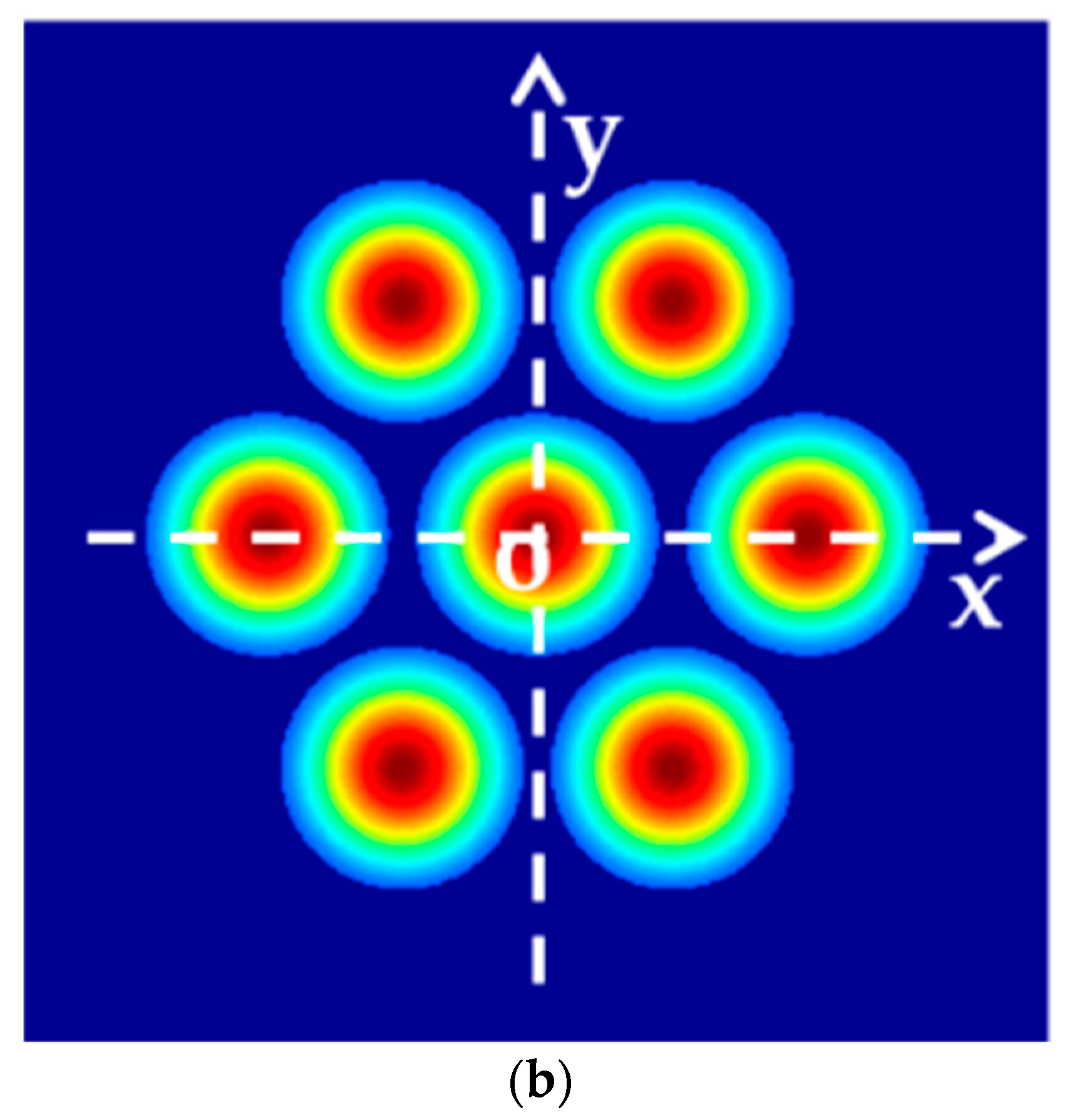
The key step of CBC is to manipulate the phase controller to make each sub-beam co-phase. In intelligent algorithms, it models the predicted piston phase through the far-field image. Then, the phase controller applies the prediction for compensation. Far-field images need to accurately reflect the information of the piston phases, which requires that the far-field image have its unique corresponding piston phase. However, piston-type phase ambiguity will leave the above requirement unsatisfied. Phase ambiguity means that different piston phases may generate the same far-field image. Figure 2 shows the examples of phase ambiguity in simulation, in which three different piston phases correspond to the same far-field image. We find that the piston phase in Figure 2c is equal to adding a common piston phase () to all sub-apertures in Figure 2a. We call this phenomenon of phase ambiguity phase redundancy. The piston phase in Figure 2e could be obtained by rotating the original piston phases in Figure 2a 180 degrees and conjugating it. We call this phenomenon of phase ambiguity rotational conjugate symmetry (this phenomenon only occurs in centrosymmetric arrays). The following discussion will prove why they generate the same far-field image and provides solutions to eliminate their impact.
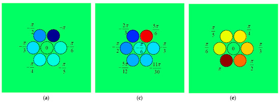
Figure 2.
Three different piston phases which can generate the same far-field. (a,b) Phase1 and its far-field. (c,d) Phase2 (adding a common phase to phase1) and its far-field. (e,f) Phase3 (rotating phase1 180 degrees and conjugating it) and its far-field.
On the emissive plane, the sub-apertures are usually arranged in a centrosymmetric shape, which is beneficial to reduce the sidelobe energy and obtain high-quality combined beams [33,34,35,36,37,38]. However, the centrosymmetric arrangement will cause phase ambiguity. Next, we discuss phase ambiguity with the example of a regular-hexagonal 7-element arrangement.
Without loss of generality, we construct a Cartesian coordinate system with the center of the emissive plane as the origin, as shown in Figure 1b. The near-field complex amplitude of the n-th sub-beam can be expressed as
where is the amplitude, ω0 is the waist radius (when the sub-beams are plane waves, ω0 can be regarded as infinity), d is the diameter of sub-apertures, and (xn, yn, 0) is the coordinate of the n-th sub-aperture’s center in the above coordinate system. . The near-field complex amplitude after piston phase modulation could be expressed as
The index of the sub-aperture at the center is 0, the corresponding piston phase is (the value range of all phases in this paper is [−π, π]), and the corresponding center coordinate is . We find that when the sub-apertures are in a centrosymmetric arrangement, for the n-th sub-aperture (n ≠ 0), there always exists another sub-aperture which is centrosymmetric with it regarding the sub-aperture 0. We denote the index of this sub-aperture as −n; the corresponding piston phase is , and the central coordinate is (x−n, y−n, 0). It is obvious that x−n = −xn and y−n = −yn. The overall near-field complex amplitude modulated by the piston phase is equal to the sum of each sub-aperture, which can be expressed as
where n = 0, ±1, ±2,…, ±(N − 1) ÷ 2. The near-field complex amplitude is transformed to the far-field complex amplitude at the focal plane by the lens. Then, the relationship between and can be expressed by the Fraunhofer diffraction formula, as follows [39].
where and ( is the wave number, λ is the beam wavelength, and is the focal length of the transform lens). If we make the variable substitution x′ = x − xn and y′ = y − yn, the far-field complex amplitude of the n-th sub-beam can be rewritten as
We separate the variables independent of x′ and y′, then move them out of the integral symbol. Equation (5) is transformed into
We denote (the value of is independent of n) and substitute Equation (6) with Equation (4). Then, we obtain the superposition of each sub-beam’s far-field complex amplitude
where (n = 0, ±1, ±2,…, ±(N − 1) ÷ 2) denotes the set of the n-th sub-beam’s piston phase. The far-field intensity distribution could be calculated from the square of the far-field complex amplitude’s modulus, which can be expressed as
The far-field intensity distribution determines the shape of the far-field image on the charge-coupled device (CCD) camera. Here, we only consider the influence of the piston phase on the far-field image, so we separate (), which is related to .
where i, j = 0, ±1, ±2,…, ±(N − 1) ÷ 2. Without loss of generality, we denote , and then a set of N pistons (n = 0, ±1, ±2,…, ±(N − 1) ÷ 2) can be expressed by a set of N − 1 relative pistons (n = ±1, ±2,…, ±(N − 1) ÷ 2). This corresponds to phase redundancy (for more details, see Appendix A). Since phase redundancy can be solved by relative phase expression, we will not consider phase redundancy during the later discussion on phase ambiguity. After substituting the relative pistons and into Equation (9), we get
where i, j = ±1, ±2,…, ±(N − 1) ÷ 2. Then, we define and (when j ≠ 0). By substituting them into Equation (10), we obtain
In a regular-hexagonal arrangement (7-element), if and generate the same far-field image, that is, , we get (for more details, see Appendix C)
If the expression of Equation (13) holds, the coefficients of and in are equal to the ones in for i =1,2,…, (N − 1) ÷ 2 (for more details, see Appendix B.). The coefficient of in is , and the coefficient of in is . The ones in are and . So, we obtain
We define . Then, (11) could be rewritten as
When and hold, we get
Equation (16) has two solutions, which are
When (17) holds, the coefficients of and in are equal to the ones in for i = 1, 2,…, (N − 1) ÷ 2. As in the analysis on (13), we have
After simultaneously solving (14) and (19), we obtain
where m is an integer. Equation (21) indicates that and may generate the same far-field image when the difference between and is an integer multiple of 2π (i = ±1, ±2,…, ±(N − 1) ÷ 2). We denote this solution of as solution 1.
Another solution of (16) is (18), which means the coefficients of and in are the opposites of the ones in for i = 1, 2,…, (N − 1) ÷ 2. As in the analysis on (19), we get
After simultaneously solving (22) and (19), we obtain
where m is an integer. We denote this solution of as solution 2. Solution 2 corresponds to a rotational conjugate symmetry, which is caused by the central symmetrical arrangement of the arrays.
The above analysis shows that there exist two different piston phases (when , these two solutions degenerate into one), which will generate the same far-field image in a 7-element system. This is the reason why it is difficult to correctly predict the piston phase with a single far-field image. In particular, solution 1 and solution 2 constitute all solutions of . If we can distinguish between solution 1 and solution 2, the phase ambiguity in a 7-element system will be solved.
2.2. Solution to Piston-Type Phase Ambiguity
According to the analysis in Section 2.1, solution 1 corresponds to the original piston phase (denoted as ), and solution 2 corresponds to the phase obtained by rotating the original piston phase 180 degrees and conjugating it (denoted as ). Therefore, and its rotationally conjugate piston phase will generate the same far-field image. This multi-solution problem is the phase ambiguity.
In CBC, it is necessary to distinguish these two situations so that we can obtain accurate information on the piston phase for phase compensation. In practice, in order to achieve this, an additional optical device needs to be added to the system, which will increase the cost of building and maintaining the experimental platform. Especially when the system is highly integrated, it is difficult to add additional optical devices. We consider distinguishing these two piston phases by breaking the rotationally conjugate symmetry in principle. We declare that applying non-centrosymmetric arrays is a choice to solve this problem, but, as mentioned earlier, it will damage the quality (the energy ratio of the central lobe) of the combined beam. Our method is to introduce phase modulation . The modulated phase can be expressed as and , where . If and generate different far-field images, the following formula holds (where m is an integer).
In fact, if , Equation (27) always holds. If (that is ), the multi solution problem no longer exists. Therefore, we only consider Equation (26). When it holds, there should be
Thus, if satisfied Equation (27), we would discriminate and () by applying a modulation phase.
We can obtain accurate information of the piston phase through a pair of far-field images. Compared with adding other optical devices (such as wavefront sensors or additional charge-coupled device (CCD) cameras on a defocus plane), our method only needs to capture a modulated image to overcome the phase ambiguity. This does not increase the complexity of the system. It should be noted that our method will take an additional step for modulated image acquisition. At the same time, it also requires the phase controller to have a high regulation accuracy to ensure the generation of a specific modulation phase.
2.3. Discussion on Scalability
We deduced all cases of phase ambiguity in a 7-element system according to the analysis in Section 2.2. In this section, we will discuss the scalability of the above theories and solutions.
The first question is whether rotational conjugate symmetry will occur in arbitrary centrosymmetric arrays. is the solution of (12) and (18), so we could obtain according to (15), which indicates that rotational conjugate symmetry exists in arbitrary centrosymmetric arrays. Equations (25) and (26) still hold after adding the phase modulation satisfying (27), indicating that our method can break the rotational conjugate symmetry in centrosymmetric arrays.
The second question is whether phase ambiguity only contains rotational conjugate symmetry in larger arrays. We give two applicable conditions. In these two cases, phase ambiguity only contains rotational conjugate symmetry. At this time, our method can still determine the correct piston phase according to far-fields.
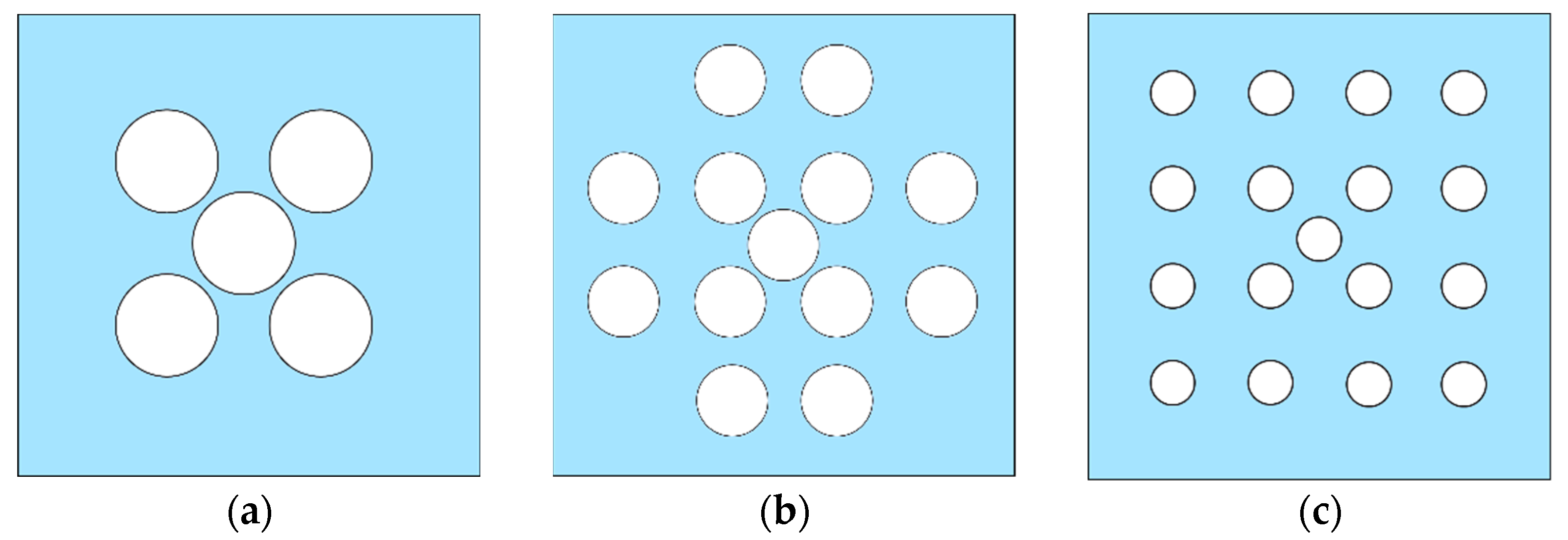
Condition 1: and do not have terms with the same frequency. The frequency of each component in can be expressed as (where i = ±1, ±2,…, ±(N − 1) ÷ 2). The frequency of each component in can be expressed as (where p, q = ±1, ±2,…, ±(N − 1) ÷ 2). Then, Condition 1 can be expressed, as for i, p, q = ±1, ±2,…, ±(N − 1) ÷ 2 does not exist. Examples of arrays meeting Condition 1 are shown in Figure 3.
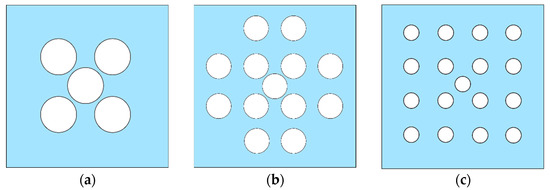
Figure 3.
Examples of the arrays which meet Condition 1. (a) 5-element. (b) 13-element. (c) 17-element.
Next, we will explain why phase ambiguity only contains rotational conjugate symmetry in arrays meeting Condition 1. When , the coefficients of each frequency component are equal (Appendix B). Thus, the coefficients of frequency in equal to the ones in . do not contain a frequency of , and so we obtain (12). Phase ambiguity contains only rotational conjugate symmetry, in this case according to the analysis in Section 2.2.
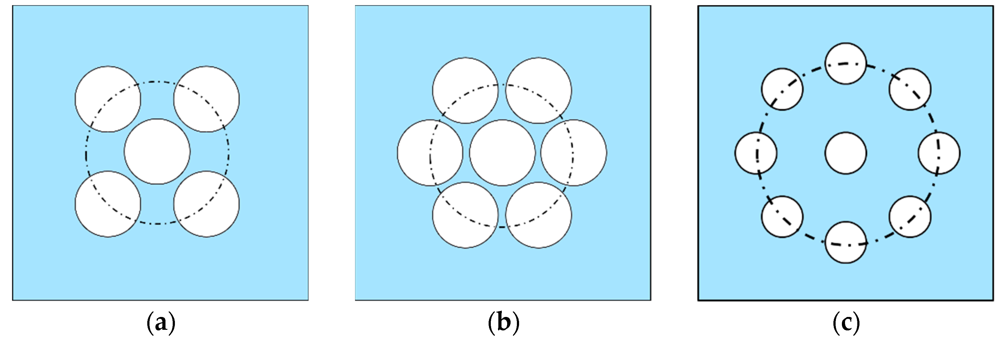
Condition 2: The centers of all sub-apertures (except sub-aperture 0) are located on the same circle (for more details and proofs, see Appendix D.). Examples of arrays meeting Condition 1 are shown in Figure 4.
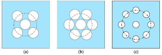
Figure 4.
Examples of the arrays which meet Condition 2. (a) 5-element. (b) 7-element. (c) 9-element.
The array arrangement affects phase ambiguity in our derivation. There is no limit on the size of sub-apertures or filling factors in Condition 1 or Condition 2, and there is no limit on the number of array elements in Condition 1 or Condition 2, which means that our method is also suitable for large-scale arrays as long as they meet one of the above conditions. The derivation process is summarized with a diagram, which is shown in Appendix E.
For more general arrangements (except for the above two cases), the frequency distribution will become very complex with the number of array elements increasing. Therefore, it will be difficult to obtain the analytical solution of phase ambiguity. Whether there exists a cause of phase ambiguity other than rotational conjugate symmetry remains to be further studied. It may be necessary to combine theoretical derivation with numerical simulation to analyze this problem. This is also the direction and focus of our future work.
3. Simulation and Result Analysis
In Section 2, we analyze the solutions of the piston phase that will cause the phase ambiguity in the CBC system with a centrosymmetric distribution of sub-apertures, and provide a method to solve this problem. In this section, we will verify our conclusions of theoretical derivation through a simulation.
We conduct simulations based on the CBC system shown in Figure 1, and the parameters are A = 1, ω0 = 11 mm, λ = 1064 nm, and . We first randomly generate 50 groups of as the Target Phase. Each group of will generate its corresponding far-field image ().
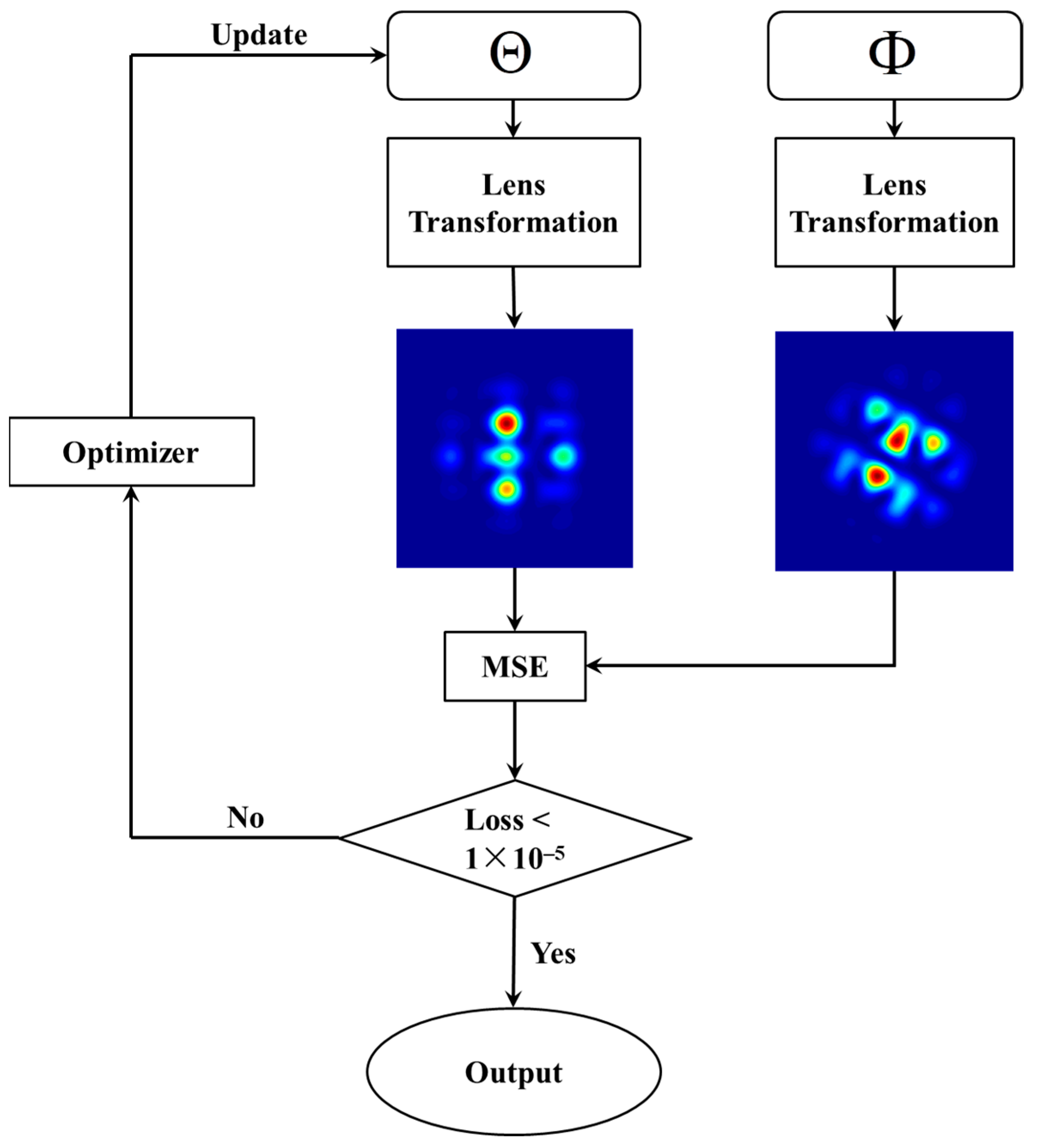
We take as the parameter and use Adam [40] for optimization. For each , we first randomly initialize the value of , then we generate its far-field image (). We calculate the mean square error (MSE) loss between normalized and , and use this loss to optimize with Adam. Then, we use the updated to generate a new far-field image and repeat the above steps.
We stopped the iteration until the loss is less than −1 ×10⁻⁵. At this time, it is considered that and generated approximately the same far-field images. The process is shown in Figure 5. It sometimes fell into the local optimum during iteration. If the loss was still more than 1 × 10⁻⁵ after 500 iterations, we would reinitialize and start a new round of iterations.
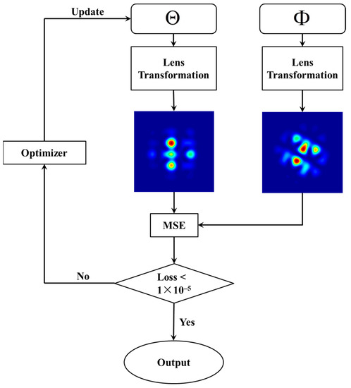
Figure 5.
The process diagram of how to find which generates the samiliar far-field to .
After obtaining a set of that meet the requirements, we would reinitialize it and repeat the above process until finding 200 groups of that have similar far-field images with . For each , we randomly initialize the value of 200 times, which means we will find 200 groups of that have far-field images similar to .
If our theoretical derivation is correct, the solutions are distributed in two intervals when the arrays meet Condition 1 and Condition 2. One is itself, and the other is ’s rotationally conjugate piston phase (). If there remain other intervals, this indicates that other solutions exist. If there exists only one interval, it means that the rotationally conjugate piston phase will not generate the same far-field image as the original one (Another possibility is that , but we avoid generating this kind of ).
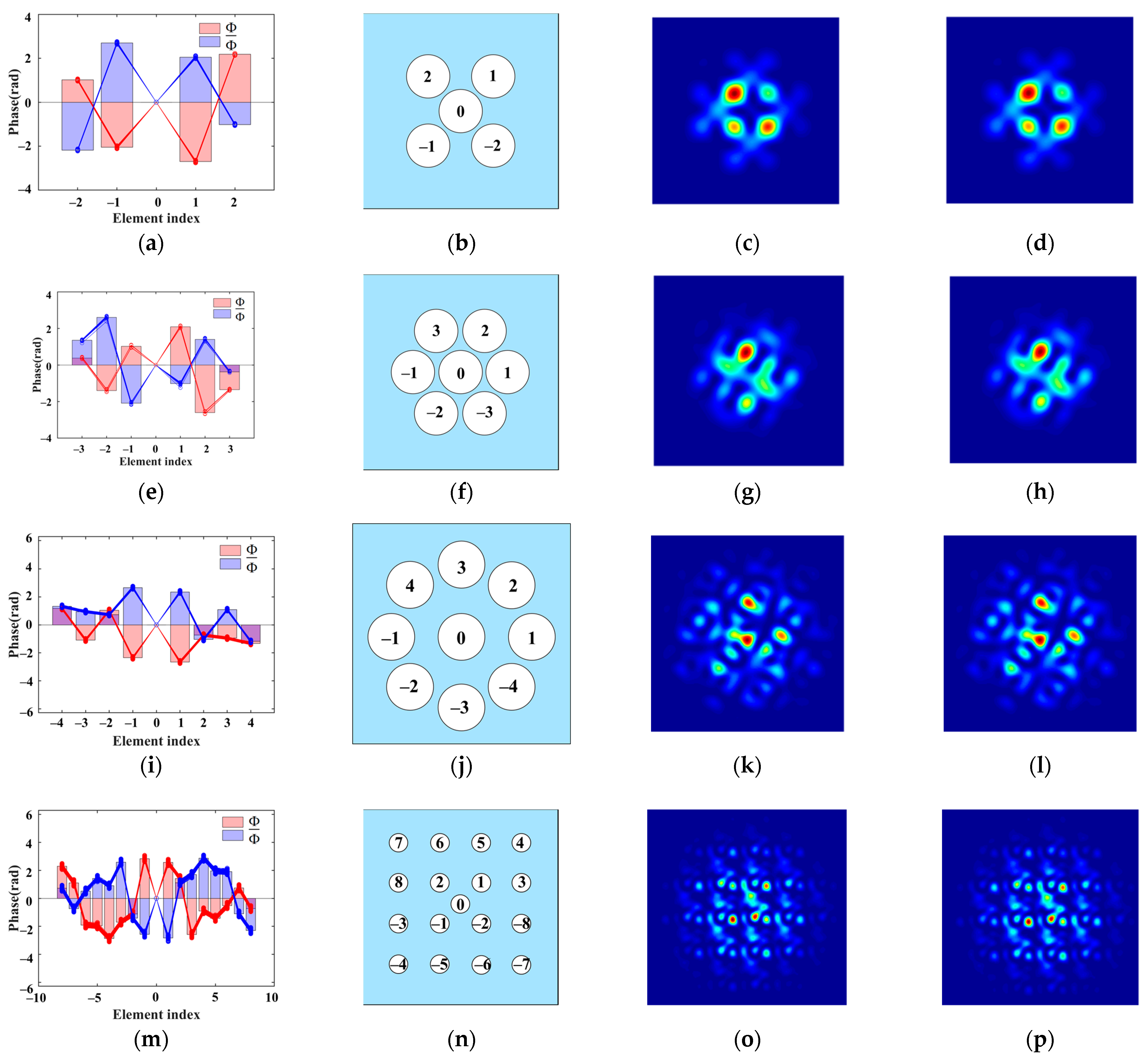
We conducted simulations, and the results demonstrate that our conclusions are correct. We randomly selected a for each system and drew the results of the above simulation iterations in Figure 6. In centrosymmetric-array CBC systems which meet Condition 1 (5-element, 7-element, and 9-element) or Condition 2 (5-element and 17-element), the solutions are distributed in two intervals (red lines and blue lines). One is itself, and the other is . Figure 4c–d,g–h,k–l and o–p show that will generate the same far-field image as .
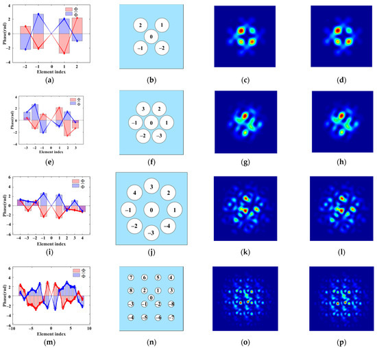
Figure 6.
(a) Solutions which generate the samiliar far field as in a 5-element system; (b) Emissive plane and element index in a 5-element system; (c) Far-field generated by in a 5-element system; (d) Far-field generated by in a 5-element system; (e) Solutions which generate the samiliar far field as in a 7-element system; (f) Emissive plane and element index in a 7-element system; (g) Far-field generated by in a 7-element system; (h) Far-field generated by in a 7-element system; (i) Solutions which generate the samiliar far field as in a 9-element system; (j) Emissive plane and element index in a 9-element system; (k) Far-field generated by in a 9-element system; (l) Far-field generated by in a 9-element system; (m) Solutions which generate the samiliar far field as in a 17-element system; (n) Emissive plane and element index in a 17-element system; (o) Far-field generated by in a 17-element system; (p) Far-field generated by in a 17-element system.
Aiming at verifying whether our method can effectively solve the phase ambiguity problem, we designed a simulation process similar to the previous one. The difference is that we not only require and to generate similar far-field images, but also the modulated ones to generate similar far-field images. The process is shown in Figure 7a.

Figure 7.
(a) In the process, we not only make generate the samiliar far-field to , but also make modulated generate the samiliar far-field to modulated ; (b) The modulation phase we use in the 5-element system; (c) The modulation phase we use in the 7-element system; (d) The modulation phase we use in the 9-element system; (e) The modulation phase we use in the 17-element system.
If our method works, the solutions are only distributed near . We can see that modulated and modulated will no longer generate the far field from Figure 8, which indicates that we can distinguish them by a pair of far-field images. The results of the simulations are consistent with our conclusions, which indicates that our method is effective.
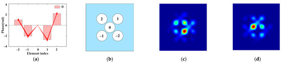
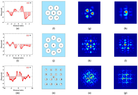
Figure 8.
(a) Solutions which generate the samiliar far field as with and without modulated in 5-element; (b) Emissive plane and element index in 5-element; (c) Modulated far-field generated by in the 5-element system; (d) Modulated far-field generated by in the 5-element system; (e) Solutions which generate the samiliar far field as with and without modulated in the 7-element system; (f) Emissive plane and element index in the 7-element system; (g) Modulated far-field generated by in the 7-element system; (h) Modulated far-field generated by in the 7-element system; (i) Solutions which generate the samiliar far field as with and without modulated in the 9-element system; (j) Emissive plane and element index in the 9-element sstem; (k) Modulated far-field generated by in the 9-element system; (l) Modulated far-field generated by in the 9-element system; (m) Solutions which generate the samiliar far field as with and without modulated in the 17-element system; (n) Emissive plane and element index in the 17-element system; (o) Modulated far-field generated by in the 17-element system; (p) Modulated far-field generated by in the 17-element system.
4. Impact of Piston-Type Phase Ambiguity
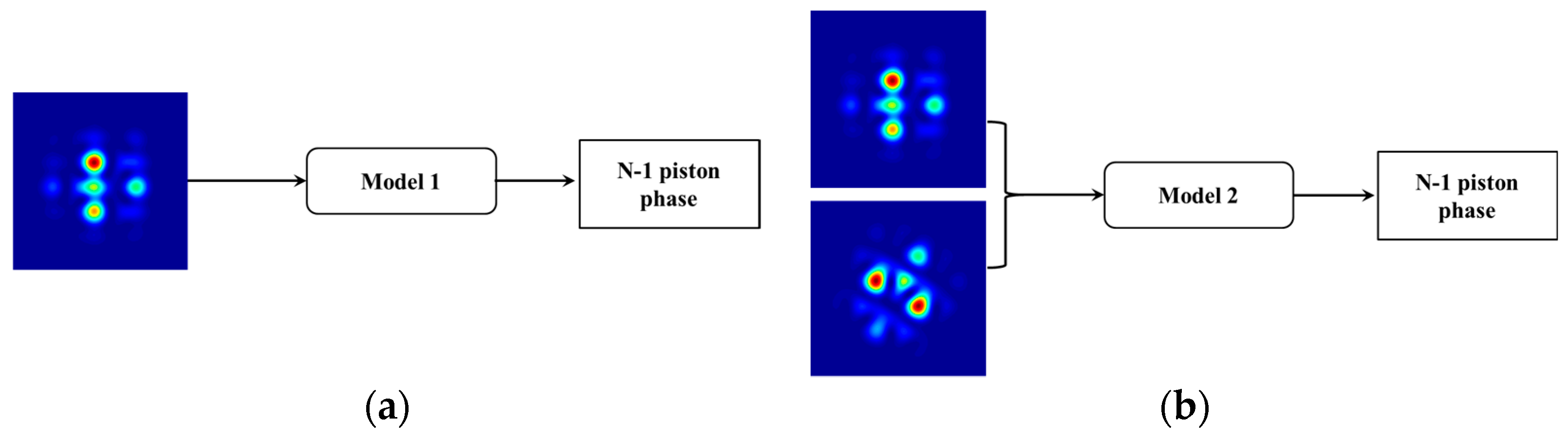
As image-based intelligent algorithms, deep learning algorithms predict the piston phase from the far-field image, and compensate the current piston phase with the prediction to realize the co-phase. Through the analysis in Section 2, we prove that there exist two piston phase distributions in centrosymmetric arrays, which may generate the same far-field image. Therefore, we cannot distinguish them from a single far-field image. In other words, this mapping relationship can be described as “one to many”. If we force the NN model to fit this relationship, it will be difficult for the model to converge. In the next part, we will show the impact of phase ambiguity through simulations.
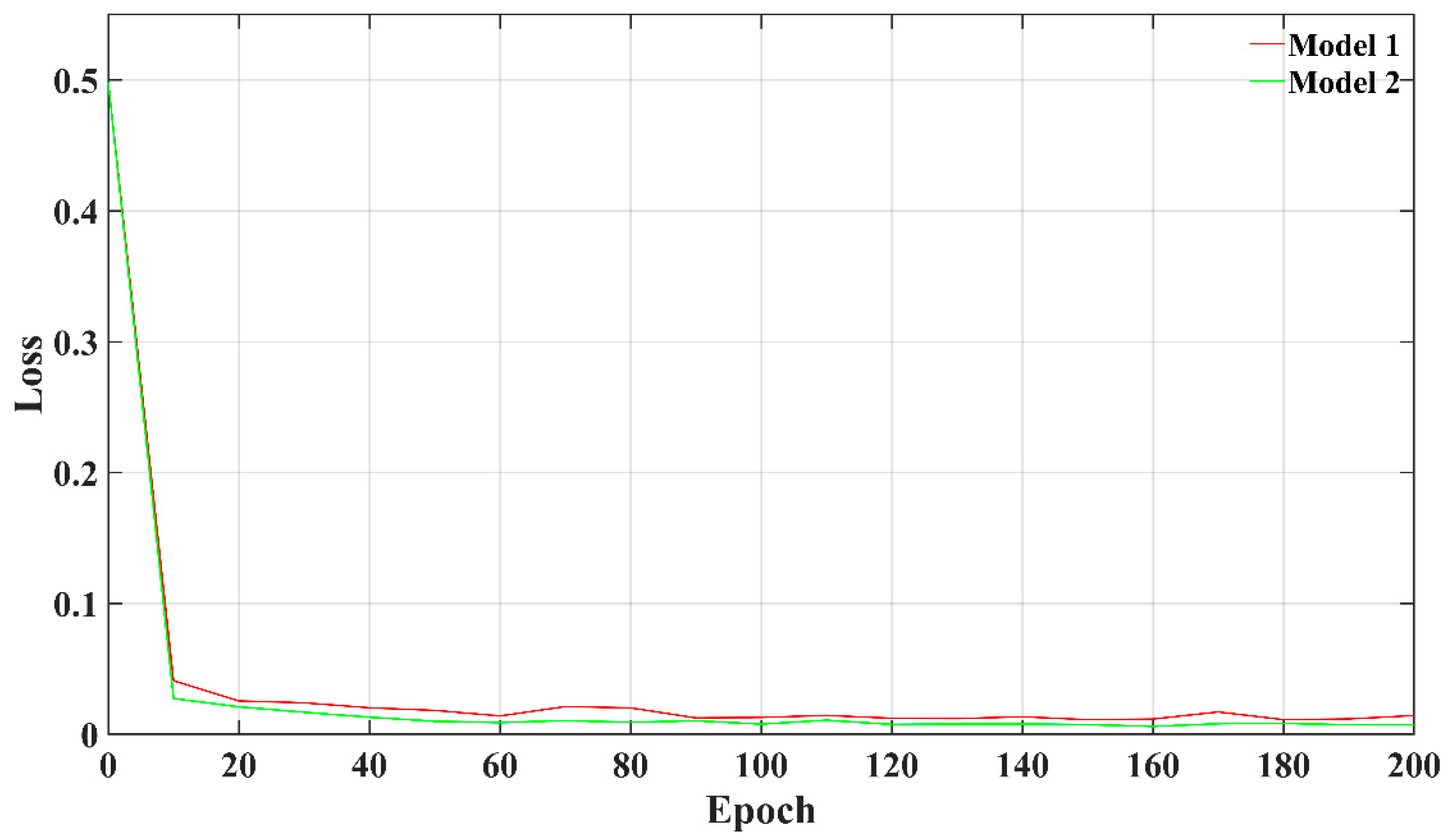
We conduct simulations on a 7-element CBC system. Our simulations are divided into two groups (as shown in Figure 9). In the first group, we employ model 1 to predict the piston phase from a single far-field image on the focal plane. According to our analysis, there exists phase ambiguity in this case. In the second group, model 2 takes the far-field image in the first group and the corresponding modulated ones as input (the modulation phase satisfies (29), which is shown in Figure 7c). The phase ambiguity problem is solved in the second group. We used 30,000 groups of training data to train the models for 200 epochs. We choose MSE as the loss function, which is defined as
where is the prediction of the n-th sub-aperture’s piston phase, and is the ground truth of the n-th sub-aperture’s piston phase (n = ±1, ±2,…, ±(N − 1) ÷ 2). The performances of these two models on the training data tend to converge after 200 epochs (shown in Figure 10).

Figure 9.
(a) Diagram of model 1; (b) Diagram of model 2.
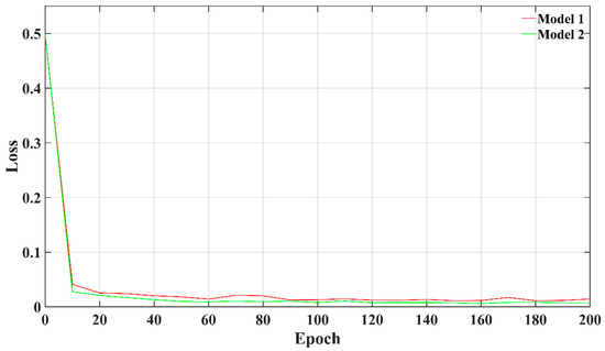
Figure 10.
Loss curves of model 1 and model 2 on the training data.
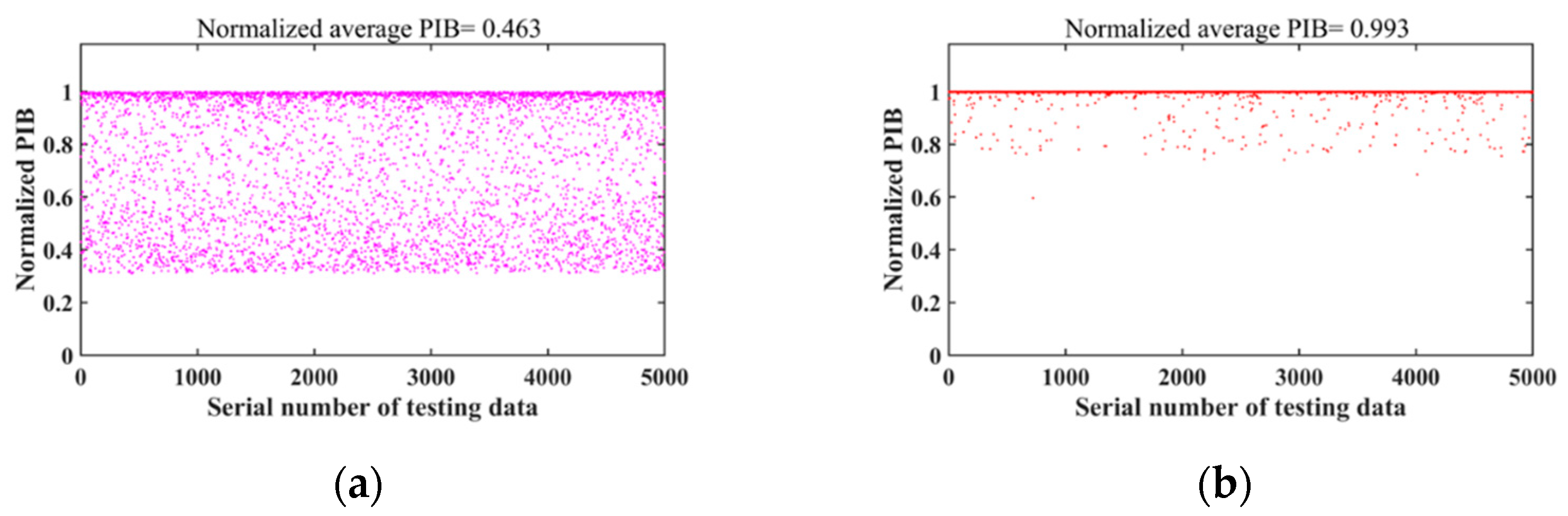
We take 5000 groups of testing data to test the performance of model 1 and model 2. We use the normalized power-in-the-bucket (PIB) as evaluation index, which can be expressed as
where is the diameter of bucket, and σ is the ideal PIB ( is 90 mm, and σ is 0.525 in our simulation). If the model performs well, its corresponding normalized PIB will be high.
The performances of model 1 and model 2 on the testing data are shown in Figure 11. Although model 1 fits the training data well, its generalization ability is poor. The result indicates that model 1 tends to “remember” rather than “infer”. The model established an unreasonable mapping relationship due to phase ambiguity, so it is difficult for model 1 to converge. Therefore, solving phase ambiguity is necessary. Model 2 performs well on both the training data and the testing data, which indicates that our method can effectively solve phase ambiguity. We submitted supplementary materials, which include the code of models and the dataset.

Figure 11.
(a) Normalized average PIB of model 1 on the testing data; (b) Normalized average PIB of model 2 on the testing data.
5. Conclusions
In this paper, we prove that piston-type phase ambiguity will occur in coherent beam combining (CBC) systems with a centrosymmetric distribution of sub-apertures. In some specific arrays, we obtain all solutions of piston-type phase ambiguity in multi-aperture CBC systems through theoretical derivation: if two groups of piston phases generate the same far-field image, they are equal or rotationally conjugate to each other. To solve this problem, we propose a method by applying asymmetric phase modulation without adding additional optical devices. In addition to the theoretical proof, we designed simulations to verify our conclusions. The simulation results show the correctness of our analysis on phase ambiguity and the effectiveness of our method. We believe that our work can not only help to theoretically analyze the corresponding relationship between the piston phase and the far-field image but also improve the performance of image-based intelligent algorithms.
Supplementary Materials
The following supporting information can be downloaded at: https://www.mdpi.com/article/10.3390/photonics9010049/s1. The dataset contains training data and testing data. Training data include 30,000 origin far-field images (named “ori32”), 30,000 modulated far-field images (named “add32”), and a label file. All images are single-channel grayscale images with 32 × 32 resolution. Each line in the label contains an image name and its corresponding 6 relative phases. As the training data, the testing data contain 5000 far-field images, 5000 modulated far-field images, and a label file. The codes for model 1 and model 2 are in two Python files (“model_1.py” and “model_2.py”). Model 1 takes origin far-field images (in “ori32”) as input. Model 2 takes both origin far-field images (in “ori32”) and modulated far-field images (in “add32”) as input. By comparing their performance on the testing data, we find that phase ambiguity will cause the non-convergence of the model.
Author Contributions
Conceptualization, H.J. and J.Z.; funding acquisition, C.G. and F.L.; methodology, H.J. and J.J.; software, H.J. and Y.L.; supervision, Q.B. and X.L.; validation, A.T. and J.R.; visualization, J.Z. and A.T.; writing—original draft, H.J. and J.Z.; writing—review & editing, Q.B. and C.G. All authors have read and agreed to the published version of the manuscript.
Funding
This research was funded by the National Natural Science Foundation of China, grant number 62175241 and 62005286.
Data Availability Statement
The dataset and the code of the models in Section 4 are available in the Supplementary Material.
Conflicts of Interest
The authors declare no conflict of interest.
Appendix A
We find that when adding a common piston phase ρ to all sub-apertures in , the value of Equation (9) remains unchanged. As shown in Figure 2, generate the same far-field image as . When the value of ρ changes, there exists an infinite number of groups of piston phases that may generate the same far field. After selecting a sub-aperture’s piston phase as the reference, we subtract the reference piston phase from the initial piston phase and obtain the relative phase. Without loss of generality, we have , and then a set of N pistons (n = 0, ±1, ±2,…, ±(N − 1) ÷ 2) can be expressed by a set of N-1 relative pistons (n = ±1, ±2,…, ±(N − 1) ÷ 2). Because of , can usually be omitted. That is, contains only the relative piston phases of N − 1 sub-apertures other than the reference one (sub-aperture 0). Unless otherwise specified, “piston phase” in the following text refers to the relative piston phase.
Appendix B
In this section, we will prove that if is a finite set of binary real numbers (if i ≠ j, and ), and for every real number u, v , then ai = αi, bi = βi for all ai, bi, αi, and βi.
First, we consider the one-dimensional case. I will introduce the following lemma.
Lemma A1.
, is a finite set of real numbers (if i ≠ j,and). For every real number u, , then pi = 0, qi = 0 for all ai, bi, αi, and βi.
We first prove Lemma A1. We divide into K1, K2, …, Km, which are pairwise disjoint. For and , when s = t, is a rational number; when s ≠ t, is an irrational number. We denote the series of elements in KS as , which can be expressed as . It is obvious that . When , we get . Because if the above formula does not hold, have periods of T1…Tm, not all equal to zero. If I ≠ j, is an irrational number. They do not have a common period, which means is not a periodic function (an example is that is not a periodic function). It is contradictory to .
Then, we consider that . If the elements in KS are rational numbers, , where , are rational numbers, signi is 0 (when is positive) or 1 (when is negative). We denote , where is a common multiple of all . Then, we have
where is a natural number. According to the uniqueness of the trigonometric series, and in KS are zeros. Then and in KS are zeros.
If the elements in KS are rational numbers, , where , are rational numbers, is an irrational number, and signi is 0 (when is positive) or 1 (when is negative). When s ≠ t, , according to the definition of KS. We denote , where is a common multiple of all . Then we have
where is a natural number. According to the uniqueness of the trigonometric series, and in KS are zeros. Then, and in KS are zeros.
For all pi and qi, we have pi = 0, qi = 0. Lemma A1 is proved.
We extend Lemma A1 to two dimensions. We denote , where is a finite set of binary real numbers (when i ≠ j, and ). We first freeze v. Then, we divide into L1, L2,…, Lm, L−1, L−2,…, L−m, which are pairwise disjointed. For and , when s = t, , which we denote as ; when s ≠ t, . Especially when s = −t, . We can rewrite as .
We denote the series consisting of the elements in Ls as .
Similarly, we denote the series consisting of the elements in L−s (if L−s exists) as .
and contain all terms of and . If , the coefficients of and are all zero according to Lemma A1. Then, we get
Then, we see v as a variable and get that all coefficients of and are zero according to Lemma A1. It should be noted that, for , there may exist or . However, due to our previous assumptions, and cannot co-exist (which avoids redundant representations).
When there exists , we denote the coefficients as and . The terms containing and are in (A5) and in (A6). When the coefficients of and in each term are zero, we get
From (A7) and (A8), we get that , , , and are all zero.
When there exists (), we denote the coefficients as and . The terms containing and are in (A5) and in (A6). When the coefficients of and in each term are zero, we get
From (A9) and (A10), we get that , , and are all zero.
If there does not exist or , we get that and are zero. Considering each term of and , we can derive that , , , and , which belong to Ls or L−s, are zero.
After repeating the above process on Lt and L−t, we finally get that all and which belong to L1, L2, …, Lm, L−1, L−2, …, L−m are 0. Therefore, the two-dimensional case is proved.
The problem at the beginning of this section is proved.
If is a finite set of binary real numbers (if i ≠ j, and ), and for every real number u, v
Then
We get ai − αi = 0 and bi − βi = 0 for all ai, bi, αi, and βi according to the above derivations.
Appendix C
The Emissive plane of the 7-element system is shown in Figure A1. We list the coordinates of each sub-aperture on the emissive plane in Table A1, which is helpful for us to analyze the frequency characteristics of the far-field image.
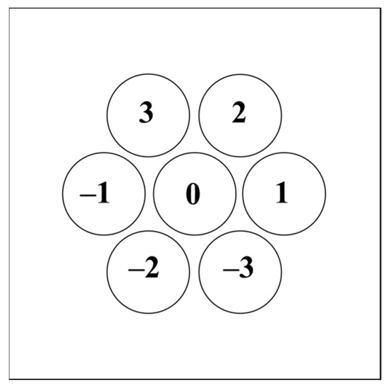
Figure A1.
Emissive plane and element index in the 7-element system.
Figure A1.
Emissive plane and element index in the 7-element system.
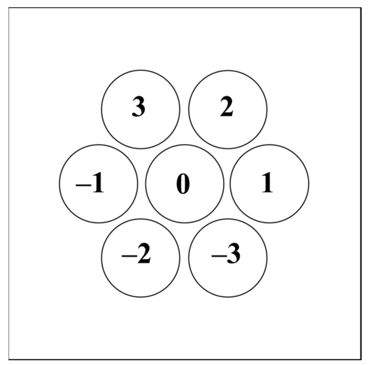

Table A1.
Coordinates of sub-apertures on the emissive plane in the 7-element system.
Table A1.
Coordinates of sub-apertures on the emissive plane in the 7-element system.
| Element Index | |||||||
|---|---|---|---|---|---|---|---|
| −3 | −2 | −1 | 0 | 1 | 2 | 3 | |
| Coordinate representation (xi, yi) | ) | ) | (−2l, 0) | (0, 0) | (2l, 0) | ) | ) |
2l is the distance from the center of sub-aperture 0 to the center of sub-aperture 1. It should be noted that the value of l will affect the shape of the far-field spot, but it will not change the solutions of phase ambiguity. By substituting (xi, yi) in Table A1 into (10), we can obtain each frequency component of the far-field image and its coefficient, which is listed in Table A2.
Table A2.
Components with different frequency and their coefficients in generated by and .
Table A2.
Components with different frequency and their coefficients in generated by and .
| Components with Different Frequency | ||
|---|---|---|
| cos (−2π(4l)u) | 2cos () | 2cos () |
| sin (−2π(4l)u) | −2sin () | −2sin () |
| cos (−2π(2l)u − 2π(2l)v) | 2cos () | 2cos () |
| sin (−2π(2l)u − 2π(2l)v) | −2sin () | −2sin () |
| cos (−2π(−2l)u − 2π(2l)v) | 2cos () | 2cos () |
| sin (−2π(−2l)u − 2π(2l)v) | −2sin () | −2sin () |
| cos (−2π(3l)u − 2π(l)v) | cos ()+ cos () | cos () + cos () |
| sin (−2π(3l)u − 2π(l)v) | sin () − sin () | sin () − sin () |
| cos (−2π(2l)v) | cos () + cos () | cos () + cos () |
| sin (−2π(2l)v) | sin () − sin () | sin () − sin () |
| cos (−2π(−3l)u − 2π(l)v) | cos () + cos () | cos () + cos () |
| sin (−2π(−3l)u − 2π(l)v) | sin () − sin () | sin () − sin () |
| cos (−2π(2l)u) | cos () + cos () + cos () + cos () | cos () + cos () + cos () + cos () |
| sin (−2π(2l)u) | sin () − sin () + sin () − sin () | sin () − sin () + sin () − sin () |
| cos (−2π(l)u − 2π(l)v) | cos () + cos () + cos () + cos () | cos () + cos () + cos () + cos () |
| sin (−2π(l)u − 2π(l)v) | sin () − sin () + sin () − sin () | sin () − sin () + sin () − sin () |
| cos (−2π(−l)u − 2π(l)v) | cos () + cos () + cos () + cos () | cos () + cos () + cos () + cos () |
| sin (−2π(−l)u − 2π(l)v) | sin () − sin () + sin () − sin () | sin () − sin () + sin () − sin () |
| 1 | 7 | 7 |
is the sum of the product of each component and its corresponding coefficient. If , the coefficients of each component are equal, according to the uniqueness of the coefficients (Appendix C.). First, because the coefficients of cos (−2π(4l)u) and sin (−2π(4l)u) are equal, we obtain
where m is an integer. As in (A14), we obtain
Then, because the coefficients of cos (−2π(3l)u − 2π(l)v) and sin (−2π(3l)u − 2π(l)v) are equal, we obtain
We introduce Lemma A2 and Lemma A3 before finding the solution of (A17).
Lemma A2.
The following formula
has 3 real solutions, which are
Next, we prove Lemma A2. By shifting the term of (A18) and applying the character of the trigonometric function, we obtain
If equals to 0, we obtain (A19) after substituting it into (A18). If is not equal to 0, we can divide both sides of (A22) by 4 and get
Substituting x in (A23) into (A18), we obtain (A20) and (A21), respectively. Lemma A2 is proved.
Lemma A3.
If one of the following formulas holds
we get
Lemma A3 is the inverse proposition of Lemma A2, which can be proved by substituting (A24), (A25), and (A26) into (A27).
Equation (A17) has three solutions according to Lemma A2. The first solution is
According to (A24) in Lemma A3, we obtain
The coefficients of cos (−2π(-l)u − 2π(l)v) and sin (−2π(-l)u − 2π(l)v) in and should be equal. When (A29) holds, we obtain
The second solution of (A17) is
According to (A15), we obtain
According to (A25) in Lemma A3, we obtain (A29) and (A30) as well.
The third solution of (A17) is
According to (A15), we obtain
According to (A26) in Lemma A3, we obtain (A29) and (A30) as well.
Similarly, we can get
(A30), (A36), and (A37) are exactly the coefficients of each component in and . Therefore, we obtain .
Appendix D
In this section, we will prove that phase ambiguity contains only rotational conjugate symmetry in circular arrays.
Since the centers of all sub-apertures (except for sub-aperture 0) are located on a circular, (where i = ±1, ±2,…, ±(N − 1) ÷ 2) can be expressed as by polar coordinates (where and ). We divide the sub-apertures into H0, H1, H2, …, Hn according to their coordinates on the emissive plane. H0 represents sub-aperture 0. Any two sub-apertures in Hj meet the condition (where m is an integer). It can also be concluded that the sub-apertures in Hj are located on the vertices of a regular hexagon.
The non-direct-current (Non-DC) frequency generated by the superposition of beams emitted from sub-apertures in H0 and Hj in the far-field can be express by a group of binary real numbers as and . represents the frequency generated by the beams from sub-aperture 0 and sub-apertures in Hj. represents the frequency generated by the beams from two sub-apertures in Hj.
The Non-DC frequency generated by the sub-apertures in Hr (r ≠ j) and Hs in the far-field image can be expressed as (when s ≠ 0) or (when s = 0).
Lemma A4.
If
holds, we obtain
According to (A38) and (A39), we obtain
After substituting b in (A42) into (A38) and (A39), we can obtain (A40) and (A41). Lemma A4 is proved.
If there exists a common frequency between and , we obtain
This is in contradiction with r ≠ j. Therefore, there does not exist a common frequency between and .
If there exists a common frequency between and , we obtain
which has 2 solutions (according to Lemma A4)
This is in contradiction with r ≠ j. Therefore, there does not exist a common frequency between and . Similarly, there does not exist a common frequency between and .
If there exists a common frequency between and , we obtain
According to Lemma A2, (A48) has three solutions
(A49) is in contradiction with Non-DC. (A50) and (A51) are in contradiction with r ≠ j. Therefore, there does not exist a common frequency between and .
In conclusion, we can see H0 and Hj as an independent system without considering the influence of other sub-apertures.
If the number of sub-apertures in Hj is 6, we obtain when , according to Appendix D (the frequency of can be expressed as ). If the number of sub-apertures in Hj is less than 6, because there is no coupling term, we obtain .
According to , we can get that (12) holds. In this case, phase ambiguity contains only the rotational conjugate symmetry referring to the analysis in Section 2.2.
Appendix E
In this section, we show our main derivation process with a diagram.

Figure A2.
The process of our main derivations.
Figure A2.
The process of our main derivations.
References
- Fan, T.Y. Laser beam combining for high-power, high-radiance sources. IEEE J. Sel. Top. Quantum Electron. 2005, 11, 567–577. [Google Scholar] [CrossRef]
- Peng, C.; Liang, X.; Liu, R.; Li, W.; Li, R. High-precision active synchronization control of high-power, tiled-aperture coherent beam combining. Opt. Lett. 2017, 42, 3960–3963. [Google Scholar] [CrossRef]
- Vorontsov, M.; Filimonov, G.; Ovchinnikov, V.; Polnau, E.; Lachinova, S.; Weyrauch, T.; Mangano, J. Comparative efficiency analysis of fiberarray and conventional beam director systems in volume turbulence. Appl. Opt. 2016, 55, 4170–4185. [Google Scholar] [CrossRef] [PubMed]
- Cheng, X.; Wang, J.L.; Liu, C.H.; Wang, L.; Lin, X.D. Fiber Positioner Based on Flexible Hinges Amplification Mechanism. J. Korean Phys. Soc. 2019, 75, 45–53. [Google Scholar] [CrossRef]
- Chen, J.; Wang, T.; Zhang, X.; Sun, Z.; Jiang, Z.; Yao, H.; Chen, P.; Zhao, Y.; Jiang, H. Free-space transmission system in a tunable simulated atmospheric turbulence channel using a high-repetition-rate broadband fiber laser. Appl. Opt. 2019, 58, 2635–2640. [Google Scholar] [CrossRef]
- Geng, C.; Li, F.; Zuo, J.; Liu, J.; Yang, X.; Yu, T.; Jiang, J.; Li, X. Fiber laser transceiving and wavefront aberration mitigation with adaptive distributed aperture array for free-space optical communications. Opt. Lett. 2020, 45, 1906–1909. [Google Scholar] [CrossRef] [PubMed]
- Liu, R.; Peng, C.; Wu, W.; Liang, X.; Li, R. Coherent beam combination of multiple beams based on near-field angle modulation. Opt. Express 2018, 26, 2045–2053. [Google Scholar] [CrossRef]
- Weyrauch, T.; Vorontsov, M.; Mangano, J.; Ovchinnikov, V.; Bricker, D.; Polnau, E.; Rostov, A. Deep turbulence effects mitigation with coherent combining of 21 laser beams over 7 km. Opt. Lett. 2016, 41, 840–843. [Google Scholar] [CrossRef]
- Su, R.; Ma, Y.; Xi, J. High-efficiency coherent synthesis of 60-channel large array element fiber laser. Infrared Laser. Eng. 2019, 48, 331. [Google Scholar]
- Adamov, E.V.; Aksenov, V.P.; Atuchin, V.V.; Dudorov, V.V.; Kolosov, V.V.; Levitsky, M.E. Laser beam shaping based on amplitude-phase control of a fiber laser array. OSA Contin. 2021, 4, 182–192. [Google Scholar] [CrossRef]
- Chang, H.; Chang, Q.; Xi, J.; Hou, T.; Su, R.; Ma, P.; Wu, J.; Li, C.; Jiang, M.; Ma, Y.; et al. First experimental demonstration of coherent beam combining of more than 100 beams. Photon. Res. 2020, 8, 1943. [Google Scholar] [CrossRef]
- Shekel, E.; Vidne, Y.; Urbach, B. 16kW single mode CW laser with dynamic beam for material processing. Fiber Lasers XVII Technol. Syst. Int. Soc. Opt. Photonics 2020, 11260, 1126021. [Google Scholar] [CrossRef]
- Prieto, C.; Vaamonde, E.; Diego-Vallejo, D.; Jimenez, J.; Urbach, B.; Vidne, Y.; Shekel, E. Dynamic laser beam shaping for laser aluminium welding in e-mobility applications. Procedia CIRP 2020, 94, 596–600. [Google Scholar] [CrossRef]
- Zhi, D.; Ma, Y.; Tao, R.; Zhou, P.; Wang, X.; Chen, Z.; Si, L. Highly efficient coherent conformal projection system based on adaptive fiber optics collimator array. Sci. Rep. 2019, 9, 2783. [Google Scholar] [CrossRef] [PubMed]
- Mailloux, R.J. Phased Array Antenna Handbook; Artech House: Norwood, MA, USA, 2017. [Google Scholar]
- Li, F.; Geng, C.; Huang, G.; Yang, Y.; Li, X. Wavefront sensing based on fiber coupling in adaptive fiber optics collimator array. Opt. Express 2019, 27, 8943–8957. [Google Scholar] [CrossRef] [PubMed]
- Vorontsov, M.A.; Kolosov, V. Target-in-the-loop beam control: Basic considerations for analysis and wave-front sensing. JOSA A 2005, 22, 126–141. [Google Scholar] [CrossRef]
- Sun, J.; Hosseini, E.S.; Yaacobi, A.; Cole, D.; Leake, G.; Coolbaugh, D.; Watts, M.R. Two-dimensional apodized silicon photonic phased arrays. Opt. Lett. 2014, 39, 367–370. [Google Scholar] [CrossRef]
- Stamnes, J.J. Waves in Focal Regions: Propagation, Diffraction and Focusing of Light, Sound and Water Waves; Routledge: London, UK, 2017. [Google Scholar]
- Shay, T.M.; Benham, V.; Baker, J.T.; Sanchez, A.D.; Pilkington, D.; Lu, C.A. Self-Synchronous and Self-Referenced Coherent Beam Combination for Large Optical Arrays. IEEE J. Sel. Top. Quantum Electron. 2007, 13, 480–486. [Google Scholar] [CrossRef]
- Ma, Y.; Wang, X.; Leng, J.; Xiao, H.; Dong, X.; Zhu, J.; Du, W.; Zhou, P.; Xu, X.; Si, L.; et al. Coherent beam combination of 108 kW fiber amplifier array using single frequency dithering technique. Opt. Lett. 2011, 36, 951–953. [Google Scholar] [CrossRef]
- Müller, M.; Aleshire, C.; Stark, H.; Buldt, J.; Steinkopff, A.; Klenke, A.; Tünnermann, A.; Limpert, J. 10.4 kW coherently-combined ultrafast fiber laser. Opt. Lett. 2020, 45, 3083–3086. [Google Scholar] [CrossRef] [PubMed]
- Chosrowjan, H.; Furuse, H.; Fujita, M.; Izawa, Y.; Kawanaka, J.; Miyanaga, N.; Hamamoto, K.; Yamada, T. Interferometric phase shift compensation technique for high-power, tiled-aperture coherent beam combination. Opt. Lett. 2013, 38, 1277–1279. [Google Scholar] [CrossRef]
- Fsaifes, I.; Daniault, L.; Bellanger, S.; Veinhard, M.; Bourderionnet, J.; Larat, C.; Lallier, E.; Durand, E.; Brignon, A.; Chanteloup, J.C. Coherent beam combining of 61 femtosecond fiber amplifiers. Opt. Express 2020, 28, 20152. [Google Scholar] [CrossRef] [PubMed]
- Vorontsov, M.A.; Sivokon, V.P. Stochastic parallel-gradient-descent technique for high-resolution wave-front phase-distortion correction. J. Opt. Soc. Am. A 1998, 15, 2745–2758. [Google Scholar] [CrossRef]
- Geng, C.; Luo, W.; Tan, Y.; Liu, H.; Mu, J.; Li, X. Experimental demonstration of using divergence cost-function in SPGD algorithm for coherent beam combining with tip/tilt control. Opt. Express 2013, 21, 25045–25055. [Google Scholar] [CrossRef] [PubMed]
- Hou, T.; An, Y.; Chang, Q.; Ma, P.; Li, J.; Huang, L.; Zhi, D.; Wu, J.; Su, R.; Ma, Y.; et al. Deep-learning-assisted, two-stage phase control method for high-power mode-programmable orbital angular momentum beam generation. Photon. Res. 2020, 8, 715. [Google Scholar] [CrossRef]
- Liu, R.; Peng, C.; Liang, X.; Li, R. Coherent beam combination far-field measuring method based on amplitude modulation and deep learning. Chin. Opt. Lett. 2020, 18, 041402. [Google Scholar] [CrossRef]
- Tünnermann, H.; Shirakawa, A. Deep reinforcement learning for tiled aperture beam combining in a simulated environment. J. Phys. Photonics 2021, 3, 015004. [Google Scholar] [CrossRef]
- Shpakovych, M.; Maulion, G.; Kermene, V.; Boju, A.; Armand, P.; Desfarges-Berthelemot, A.; Barthélemy, A. Experimental phase control of a 100 laser beam array with quasi-reinforcement learning of a neural network in an error reduction loop. Opt. Express 2021, 29, 12307–12318. [Google Scholar] [CrossRef]
- Harvey, J.E.; Rockwell, R.A. Performance Characteristics of Phased Array And Thinned Aperture Optical Telescopes. Opt. Eng. 1988, 27, 279762. [Google Scholar] [CrossRef]
- Baron, F.; Cassaing, F.; Blanc, A.; Laubier, D. Cophasing a wide field multi-aperture array by phase-diversity: Influence of aperture redundancy and dilution. Astron. Telesc. Instrum. 2003, 4852, 663–673. [Google Scholar] [CrossRef]
- Zhang, D.; Zhang, F.; Pan, S. Grating-lobe-suppressed optical phased array with optimized element distribution. Opt. Commun. 2018, 419, 47–52. [Google Scholar] [CrossRef]
- Lei, J.; Yang, J.; Chen, X.; Zhang, Z.; Fu, G.; Hao, Y. Experimental demonstration of conformal phased array antenna via transformation optics. Sci. Rep. 2018, 8, 3807. [Google Scholar] [CrossRef] [Green Version]
- Wang, H.; He, B.; Yang, Y.; Zhou, J.; Zhang, X.; Liang, Y.; Sun, Z.; Song, Y.; Wang, Y.; Zhang, Z. Beam quality improvement of coherent beam combining by gradient power distribution hexagonal tiled-aperture large laser array. Opt. Eng. 2019, 58, 066105. [Google Scholar] [CrossRef]
- Zhi, D.; Zhang, Z.; Ma, Y.; Wang, X.; Chen, Z.; Wu, W.; Zhou, P.; Si, L. Realization of large energy proportion in the central lobe by coherent beam combination based on conformal projection system. Sci. Rep. 2017, 7, 2199. [Google Scholar] [CrossRef] [PubMed]
- Zuo, J.; Li, F.; Geng, C.; Zou, F.; Jiang, J.; Liu, J.; Yang, X.; Yu, T.; Huang, G.; Fan, Z. Experimental Demonstration of Central-Lobe Energy Enhancement Based on Amplitude Modulation of Beamlets in 19 Elements Fiber Laser Phased Array. IEEE Photonics J. 2021, 13, 1500113. [Google Scholar] [CrossRef]
- Dolph, C.L. A Current Distribution for Broadside Arrays Which Optimizes the Relationship between Beam Width and Side-Lobe Level. Proc. IRE 1946, 34, 335–348. [Google Scholar] [CrossRef]
- Goodman, J.W. Introduction to Fourier Optics; McGraw-Hill: New York, NY, USA, 2003; ISBN 978-0071142571. [Google Scholar]
- Kingma, D.P.; Ba, J. Adam: A Method for Stochastic Optimization. arXiv, 2015; arXiv:1412.6980. [Google Scholar]


Publisher’s Note: MDPI stays neutral with regard to jurisdictional claims in published maps and institutional affiliations. |
© 2022 by the authors. Licensee MDPI, Basel, Switzerland. This article is an open access article distributed under the terms and conditions of the Creative Commons Attribution (CC BY) license (https://creativecommons.org/licenses/by/4.0/).