Spatially Separated Heterodyne Grating Interferometer for In-Plane and Out-of-Plane Displacement Measurements

Abstract

Grating interferometers that measure in-plane and out-of-plane displacements are not only effective two-degree-of-freedom (DOF) sensors, but are also basic units of six-DOF measurement systems. Besides resolution and accuracy, periodic nonlinear errors, misalignment tolerance, and size of reading heads are more crucial than ever. In this work, a spatially separated heterodyne grating interferometer that measures in- and out-of-plane displacements is proposed. A prototype with 3 mm diameter beams with a size of 69 mm × 51 mm × 41 mm was built and tested. The experiment results show that the 30 s stability is 2.5 nm; the periodic nonlinear errors of the two measuring directions are less than the resolutions (0.25 nm for in-plane motions and 0.15 nm for out-of-plane motions). Double-diffracted configuration ensures that the misalignment tolerances are three axes larger than ±2 mrad.

1. Introduction

Grating interferometers have the advantage of being insensitive to the air refractive index, attracting significant attention in precise displacement measurements, especially for multiple degree-of-freedom (DOF) measurements. Two-DOF grating interferometers that measure in-plane and out-of-plane displacements are used as basic units of six-DOF measurement systems for various stages in photolithography machines [1,2]. Therefore, research on two-DOF grating interferometers has increased in recent years [3,4,5]. Beside resolution and accuracy, periodic nonlinear errors, misalignment tolerance, and size of reading heads are crucial in two- and multiple-DOF applications.

There are two main approaches to the addition of out-of-plane displacement measurements to a grating interferometer, as we mentioned in a previous review [6] and these include building a laser interferometer or decoupling its phase from interference signals. For the former, taking Hsieh’s interferometer [7] as an example, zeroth-order diffracted beams are used as measurement beams for the laser interferometer. However, the reflected zeroth-order beam is sensitive to the roll and yaw angles of the planar grating, leading to a misalignment angle as large as twice the rotated angles. In addition, the configurations of laser and grating interferometers are difficult to miniaturize. For the latter, taking Li’s interferometer [8] as an example, the in- and out-of-plane displacements are decoupled from phases of measurement beams. Thus, out-of-plane motion measurements share the same misalignment tolerance as the in-plane measurements.

In our previous work on spatially separated heterodyne grating interferometers, the spatially separated structure is proven to eliminate the periodic nonlinear errors caused by optical mixing, removing a barrier to nanometer-scale measuring accuracy [9,10]. In addition, the double-diffracted configuration is involved in increasing the resolution and improving the misalignment tolerances to the scale of several mrad [10,11]. The double-diffraction configuration also leads to a more complicated optical configuration. However, the laser wavelength for out-of-plane motion measurements is sensitive to the fluctuations of the air refractive index. To achieve high accuracy of the complicated grating interferometer, the length of the beam path should be as short as possible. Therefore, the miniature design of the optical configuration is crucial for in- and out-of-plane grating interferometers and is an important technical issue in the field.

Small optical components will limit the beam diameter, leading to a small misalignment tolerance. Thus, to maintain large misalignment tolerance in a miniatured optical configuration, we proposed a spatially separated heterodyne grating interferometer that measures in-plane and out-of-plane displacements with 3 mm diameter beams with a size of 69 mm × 51 mm × 41 mm. The proposed grating interferometer uses a monolithic prism for compact design, which is advantageous due to its small size and good stability. The experimental results show the periodic nonlinear errors are less than 0.25 nm; the measuring accuracies of in-plane and out-of-plane are higher than 5 nm; the misalignment tolerances are larger than ±2 mrad.

2. Optical Structure and Measuring Principle

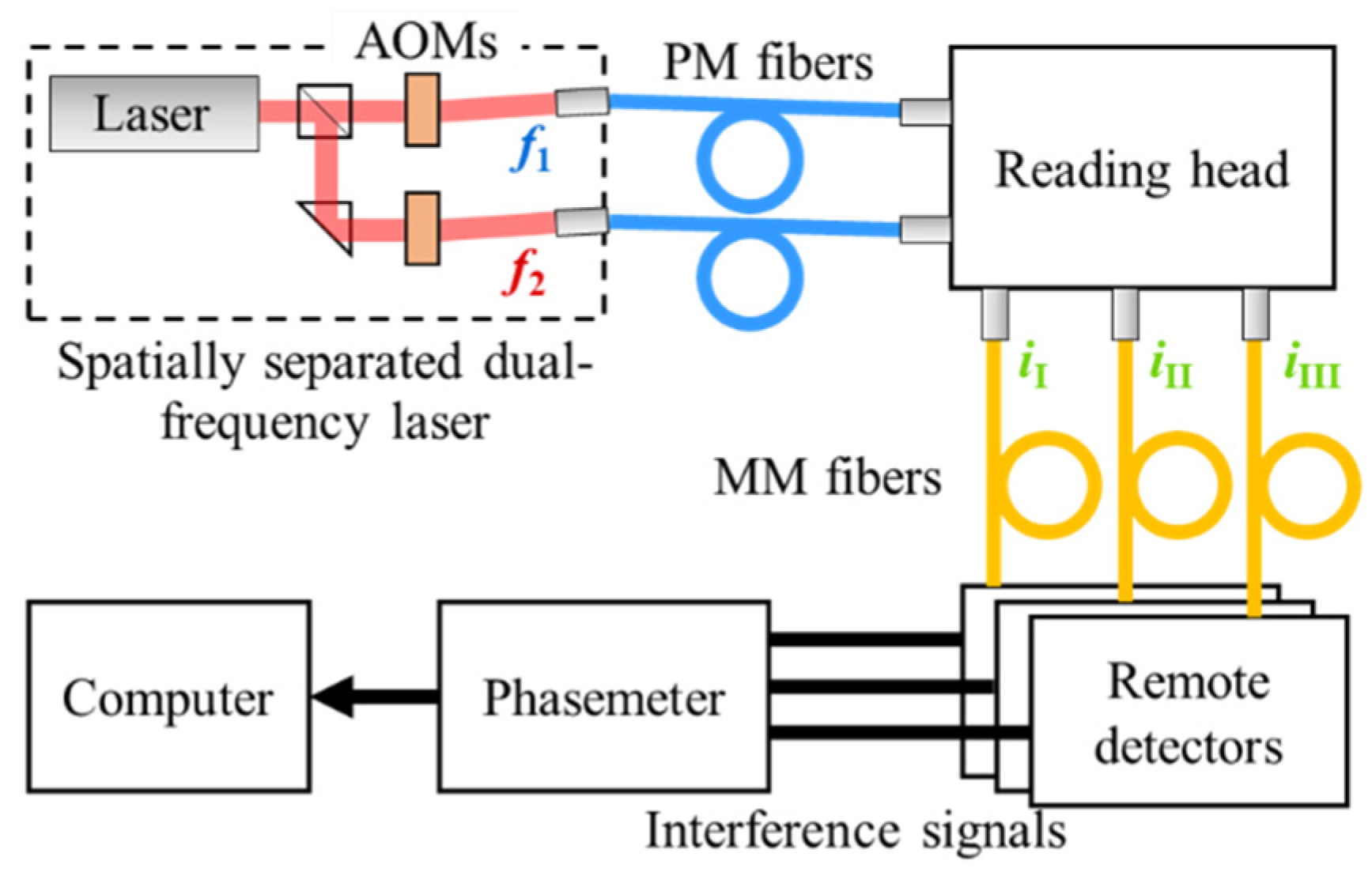
The schematic of the proposed spatially separated heterodyne grating interferometer is shown in Figure 1. A stabilized laser source with two acoustic-optical modulators is used as a spatially separated dual-frequency laser. Two laser beams, the frequencies of which are denoted as f₁ and f₂, are transmitted to the reading head via individual polarization-maintaining optical fibers. Then, three interference beams generated at the reading head are transmitted to remote detectors. A phasemeter is used for decoupling and calculating the displacements from the phases of interference signals.

Schematics of the optical configuration of the reading head that illustrate the principle and structure are shown in Figure 2. As Figure 2a shows, the optical configuration is composed of a center beam splitter (CBS), a lateral displacement beam splitter (LDBS), and three retro-reflectors (RRs) for one reference beam and two measurement beams.

The CBS contains two beam-splitting surfaces—a polarized one that lies on the diagonal surface of the cube and a non-polarized one that is located on the middle-line surface of the lower triangular prism. The split and combination of these beams are carried out in the CBS with the help of the retro-reflector RR₀, which substitutes the 45° angle-placed beam-combining beam splitters in the previous work [10,11].

As depicted in Figure 2a, two modulated beams with frequencies f₁ and f₂ (assuming f₁ > f₂) emitted from two fiber collimators (not shown) enter the CBS and are split into two parts at the polarized splitting surface, respectively. The reflected s-polarized beams are transferred to the RR₀ and are reflected. We ignored the initial phase and assumed that the wave equations of these beams are as follows:

$$E_1\propto \cos \left(2\pi f_{1}t\right)$$

(1)

$$E_2\propto \cos \left(2\pi f_{2}t\right)$$

(2)

where t is time.

As the name indicates, there are two diffraction steps that occur in the double-diffraction optical configuration. The transmitted p-polarized beams of CBS transfer to the grating interferometer and diffract (the first-step diffractions). The incident angles of the first diffractions are 90 degrees. The diffracted beams, +1st-order of f₁ beam and −1st-order of f₂ beam, are returned by the corresponding retro-reflectors RR₁ and RR₂, and then the second step of diffractions occur. A pair of the diffracted beams of the second diffractions, (+1,+1)-order of the f₁ beam and (−1,−1)-order of the f₂ beam, are in parallel with the incident beams of the first diffractions, but are transmitted away from the grating. Except for the aforementioned diffracted beams, other orders of diffracted beams are not involved in the measurement. Considering the optical Doppler frequency shifts caused by in-plane motion of the grating and the changes in optical paths caused by out-of-plane motion, the second diffracted beams are expressed as

$$E_3\propto \cos \left[2\pi \left(f_1+2\mathrm{\Delta }{f}_x+k\mathrm{\Delta }{f}_z\right)t\right]$$

(3)

$$E_4\propto \cos \left[2\pi \left(f_2-2\mathrm{\Delta }{f}_x+k\mathrm{\Delta }{f}_z\right)t\right]$$

(4)

In Equations (3) and (4), the factor 2 before Δf_x is induced by the double-diffracted configuration, which means a doubled optical fold factor. The factor k is determined by the geometric scheme of the incident and diffracted beams, which will be further discussed in the following sections. The Doppler frequency shifts Δf_x and Δf_z are determined by the moving velocity v_x and v_z, and the corresponding benchmarks—the pitch d of the grating and the wavelength λ of the laser.

$$\mathrm{\Delta }{f}_x=\frac{v_x}{d}$$

(5)

$$\mathrm{\Delta }{f}_z=\frac{v_z}{\lambda }$$

(6)

Then, the returned s-polarized beams and the second diffracted p-polarized beams combine at the polarized splitting surface of the CBS. Because the output beams and the input beams are centrally symmetric, the two combined interfering beams can be calculated by adding E₁ and E₄, E₂ and E₃, respectively. Thus, the alternating intensities detected by photodiodes are expressed as

$$i_1=E_1+E_4\propto \cos \left[2\pi \left(f_1-f_2+2\mathrm{\Delta }{f}_x-k\mathrm{\Delta }{f}_z\right)t\right]$$

(7)

$$i_2=E_2+E_3\propto \cos \left[2\pi \left(f_1-f_2+2\mathrm{\Delta }{f}_x+k\mathrm{\Delta }{f}_z\right)t\right]$$

(8)

Although the intensities in Equations (7) and (8) include the phases caused by in- and out-of-plane motions, only the out-of-plane displacement along the z-axis could be calculated because there are three variables with two functions. Therefore, a third signal generated by the non-polarized beam-splitting surface in the CBS is needed for measuring x-axis displacement.

As shown in Figure 2a, the second diffracted beams are split into the following two parts: the transmitted part analyzed above, and the reflected part combined with an LDBS. Then, we obtain the expression for the third interfering beam, which is as follows:

$$i_3=E_3+E_4\propto \cos \left[2\pi \left(f_1-f_2+4\mathrm{\Delta }{f}_x\right)t\right]$$

(9)

Assuming the phases of the signals i₁ through i₃ are φ₁, φ₂, and φ₃, and by substituting the phases in beat frequency and Doppler frequency shift with φ_beat, φ_x and φ_z, shown by

$$\{\begin{array}{l}{\phi }_{beat}=2\pi \left(f_1-f_2\right)t\\ {\phi }_x=2\pi \mathrm{\Delta }{f}_{x}t\\ {\phi }_z=2\pi \mathrm{\Delta }{f}_{z}t\end{array}$$

(10)

a set of linear equations with three variables can be obtained to calculate the displacements.

$$\{\begin{array}{l}{\phi }_1={\phi }_{beat}+2{\phi }_x-k{\phi }_z\\ {\phi }_2={\phi }_{beat}+2{\phi }_x+k{\phi }_z\\ {\phi }_3={\phi }_{beat}+4{\phi }_x\end{array}$$

(11)

The equations can be solved after using a phasemeter to acquire three phases φ₁, φ₂, and φ₃, and the displacements x and z are converted as follows:

$$4x=\frac{{\phi }_x}{2\pi }d$$

(12)

$$kz=\frac{{\phi }_z}{2\pi }\lambda$$

(13)

As Figure 2b shows, the structure of the reading head is carefully designed. The beam paths are arranged in a three-dimensional configuration to reduce the size of the reading head. The retro-reflectors RR₀ and LDBS are directly attached to the CBS by optical adhesive, forming a monolithic beam-splitter prism. The monolithic design is advantageous for short beam paths in the air, which leads to better stability. RR₁ and RR₂ are independent of the monolithic prism, which is helpful when assembling and adjusting the reflectors.

The z-axis displacement measurement factor can be further calculated from the structure. Taking one part of the beams as an example, when the grating occurs along the z-direction as Figure 3 shows, the optical path extends and the spots on the surface of RR deviate. The red dashed lines represent the extended path. Since the output of the RR is centrally symmetric, the two green-shaded triangles in the projection view are congruent, which means that the total extension l in the first and second diffracted beams are equal to the equation

$$l=2z\left(1+\frac{1}{\cos \theta }\right)=kz$$

(14)

where the diffracted angle θ is determined by the grating equation. In addition to the exact value of the factor k, Equation (14) also proves that the double-diffracted configuration doubles the fold factor of measuring displacements in both x- and z-directions.

3. Prototype and Experiments

3.1. Prototype of the Reading Head

Spatially separated heterodyne interferometry and double diffraction are both complicated configurations. The most significant problem in design is that a thick beam leads to larger misalignment tolerances, but requires larger prisms for clear apertures. The prism and reading head were elaborately designed to reduce their size. Pictures of the monolithic prism and the prototype are shown in Figure 4. As Figure 4a shows, the RR₀ and LDBS are attached to a 15 mm CBS. Beam diameters are 3 mm. A monolithic prism is advantageous because of its smaller size and shorter optical path in the air. Figure 4b shows the prototype of the reading head, whose fiber collimators/couplers are adjusted and attached to the mechanical part. The size of the prototype is 69 mm × 51 mm × 41 mm. Two right-angle prisms are used for reflecting the beams towards the fiber collimators/couplers. Thinner optical collimators/couplers may closely mount or directly adhere to the CBS, which could further reduce the size of the prototype. However, thinner beams and smaller apertures will lead to worse misalignment tolerances. It is an important feature of the direction of future work, which will be discussed in Section 4.

3.2. Experimental Setup

The experimental setup is shown in Figure 5. As Figure 5a shows, a semiconductor laser (Sacher Lasertechnik Group, model: TEC500) was used to provide a stabilized-frequency laser beam with a wavelength of 781.5 nm (nominal 780 nm). Two parts of the laser beam that were divided by a beam splitter were modulated by two acoustic-optomodulators, generating a beat frequency at 5.000 MHz. Then, the beams were coupled with polarization-maintaining optical fibers.

Figure 5b shows the measurement and motion systems of the experiment setup. A positioning stage (BOCI Company, model: MTMS103) and a heterodyne laser interferometer were used to test the mm level measuring ability. A piezo-stage (Physik Instrumente, model: P-587.6) and its built-in capacitive sensors were used to test the accuracy and stability. Interference beams of the proposed grating interferometer and referencing laser interferometer were detected by remote detectors and self-developed phasemeters. Displacement results were recorded by computer via USB interfaces. The interpolation factor of the phasemeter was 1024. The diffraction angle of the 781.5 nm laser at 1 μm grating was about 51.4°. The resolutions of the x- and z-axes were 0.25 and 0.15 nm, respectively.

3.3. Test of Measurement Performance

3.3.1. Measurement Results of 2-DOF Large Displacement

The positioning stage moves along a rectangular path and the long and short sides of the stage are parallel to the x- and z-axes, respectively. The x-axis displacement is 50 mm; the z-axis displacement is 0.5 mm. The two tracks in Figure 6 that represent the proposed grating interferometer and the referencing laser interferometer correspond with each other. Displacements and differences in the two directions are shown in Figure 7. As Figure 7a shows, the average speed of x-axis motion is 5 mm/s, and the difference between the grating interferometer and the laser interferometer is ±12.5 μm. As Figure 7b shows, the average speed of z-axis motion is only 0.5 mm/s, and the difference between the grating interferometer and the laser interferometer is ±5 μm. The difference is mainly caused by vibration, straightness of the positioning stage, and Abbe error. It is for this reason that the difference became larger as the speed increased. The deviation between the start and the end positions of the entire path is less than 2.5 μm, which is less than the positioning accuracy (5 μm) of the stage.

3.3.2. Measurement Results of 2-DOF Small Displacement

Small displacements on a μm and nm scale are generated by the piezo stage. As Figure 8a shows, 100 μm diameter circular curves measured by the proposed grating interferometer and the built-in capacitive sensors correspond with each other. Their differences shown in Figure 8b are reported as ±0.2 μm. The differences are mainly caused by vibration and shaking of the hinges when the grating moves.

In the next experiment, 5 nm steps in two directions are carried out and measured. Large fluctuations that ranged across tens of nanometers could be observed in unfiltered curves, which are mainly caused by mechanical and electronic noises. Mean filtering is a commonly used method for handling high-frequency noises [12]. A window of 0.2 s is selected as the filter. As Figure 9 shows, filtered curves reveal that the proposed grating interferometer could distinguish between the 5 nm steps, which proves that the measurement accuracies for both x- and z-axes of the prototype are better than 5 nm.

Stability and fluctuations are further investigated. Taking the x-axis as an example, the results and the frequency spectrum of the stability test are shown in Figure 10. As Figure 10a shows, the range of the filtered curve in 30 s is 2.5 nm. The range of the unfiltered curve is about 25 nm and the frequency spectrum is shown in Figure 10b. Two peaks at 100 Hz and 90 Hz are found in the middle of the spectrum.

For comparison, the results of the stability test and frequency-domain analysis of the piezo stage are shown in Figure 11. Limited by the RAM capacity of the controller, the period is only 13 s. As Figure 11a shows, even if the piezo stage is expected to be stable, a ±6 nm fluctuation is detected by its capacitive sensor. The corresponding spectrum is shown in Figure 11b. The peak at 100 Hz is the main component; the peak at 90 Hz can also be found. By comparing and combining the results in Figure 10 and Figure 11, the reason for the fluctuation is that the heavy grating on the hinges is sensitive to vibrations. The reading head is further from the hinge than the capacitive sensors; therefore, the vibration is amplified.

3.4. Test of Periodic Nonlinear Errors

Periodic nonlinear errors caused by optical mixing [13] are usually as large as several nanometers. It is difficult to separate and observe the period nonlinear errors in time-domain results. Thus, frequency spectrum analysis is widely used in testing periodic nonlinear errors [14]. When the grating moves, the frequency-domain method uses the amplitude difference between the base peak and the highest peak to calculate periodic nonlinear errors. The periodic nonlinear errors Δx are also determined by the benchmark of the measurement [14,15].

$$\mathrm{\Delta }x=\frac{M\cdot {10}^{-\frac{\mathrm{\Delta }B}{20}}}{2k\pi }$$

(15)

where ΔB is the amplitude difference, k is the corresponding factor of optical Doppler frequency shifts, and M represents the benchmark. For grating interferometers, M is the grating pitch; for laser interferometers, M is the wavelength.

The schematic of the experimental setup is shown in Figure 12. A Keysight N9010A signal analyzer is used to record the frequency spectrum of the signals. In contrast to Ref. [14] and previous work [10], there are two benchmarks in one signal. Thus, the experiment is designed to be carried out in two parts, including testing the frequency spectrum of x- and z-axis motion in order. When the grating moves along the x-axis, the benchmark M in Equation (15) is 1 μm; when it moves along the z-axis, the M in Equation (15) is 780 nm.

The positioning stage is moved along the x- and z-axes, respectively. For both motions, three interference signals are sequentially acquired and analyzed by the frequency spectrum analyzer. According to Equation (11), interference signals 1 and 2 are related to motions along the x- and z-axes, while interference signal 3 only includes the phase of motion along the x-axis. Thus, five frequency spectrum curves are shown in Figure 13.

When the grating is held stable, the peak of the base signal is −25.39 dB @ 5.0008 MHz. The threshold of noises is −80 dB. As Figure 13a–c show, when the grating moves along the x-axis, the frequency shifts of signals 1 and 2 are ±6.0 kHz, while the shift of signal 3 is 11.6 kHz. No other peaks exist in the spectrum. The amplitudes of the peaks are as follows: −29.22 dB, −28.05 dB, and −25.47 dB, respectively. By using the lowest amplitude for the calculations, the periodic nonlinear error of the x-axis measurement is no larger than 0.23 nm. As Figure 13d,e show, when the grating moves along the z-axis, the frequency shifts of signals 1 and 2 are 5.2 kHz. No other peaks exist in the spectrum. The amplitudes of the peaks are as follows: −29.50 dB and −28.61 dB, respectively. Thus, the periodic nonlinear error of the z-axis measurement is no larger than 0.15 nm. The periodic nonlinear errors are less than the corresponding resolution, proving that the spatially separated configuration in the two-DOF design is effective.

3.5. Test of Misalignment Tolerance

Tips and tilts always occur in the motions of the grating. Unexpected rotations may lead to mismatches of interference beams. Therefore, misalignment tolerance is an important feature of a two-DOF grating interferometer, especially for the those in multi-DOF applications. It usually requires 2.5 mrad tolerance around three rotation axes for wafer stages in photolithography machines.

The schematic of the experimental setup is shown in Figure 14. The setup uses two autocollimators (Möller-Wedel, model: ELCOMAT 3000) to monitor the attitude of the grating and a signal analyzer to measure the residual intensities of the interference signals. The grating was assembled on a manual six-DOF motion stage to generate ±2 mrad rotations around three axes.

Before the experiments, the grating is adjusted to the optimum attitude with the highest peak. This attitude is regarded as the origin of the rotations. Then, attenuations of the peaks are recorded when the grating is rotated in steps of 10 arcsecs.

According to the optical configuration shown in Figure 1, the optical path of interference beams 1 and 2 are symmetric; their misalignment tolerances are the same. Thus, six curves of interference beams 1 and 3 are shown in Figure 15. As Figure 15a–c show, the attenuations of interference beam 1 are −3 dB, −6.5 dB, −4 dB, respectively; as Figure 15d–f show, the attenuations of interference beam 3 are −4 dB, −7dB and −4 dB, respectively. The dynamic range of the photodetectors is 6:1 (−8 dB) to 25:1 (−14 dB). The attenuation values are within the dynamic range, which means that the misalignment tolerance of the prototype is larger than ±2 mrad.

4. Discussion

Tips and tilts always exist in actual translational motion. With regard to grating interferometers, the roll, pitch, and yaw angles conventional represent the rotation around the x-, y-, and z-axis. Those three angles are shown in Figure 16.

For grating interferometers, tips and tilts on a μrad to mrad scale are influencing by two aspects, misalignments and extra phases. The misalignments will cause a decrease in the signal-to-noise ratio, resulting in an increase in random errors. This could be solved by designing an optical configuration with high misalignment tolerances, similar to the configuration we introduced in the above sections. The extra phases are caused by changes in the length of optical paths.

When the grating rotates, the phases of x- and z-axis displacements from different beams could be distinguished as φ_x1 and φ_x2, φ_z1 and φ_z2, respectively. Similar to the derivation in Section 2, we can now obtain the phase functions with rotation.

$$\{\begin{array}{l}{\phi }_1={\phi }_{beat}+2{\phi }_{x1}-k{\phi }_{z1}\\ {\phi }_2={\phi }_{beat}+2{\phi }_{x2}+k{\phi }_{z2}\\ {\phi }_3={\phi }_{beat}+2\left({\phi }_{x1}+{\phi }_{x2}\right)+k\left({\phi }_{z1}-{\phi }_{z2}\right)\end{array}$$

(16)

Using the same solutions from Equation (11) to Equations (12) and (13), the following expressions can be obtained:

$$\{\begin{array}{l}4x^{\prime }=\frac{d}{2\pi }\left[\frac{\left({\phi }_{x1}+{\phi }_{x2}\right)}{2}+\frac{3k\left({\phi }_{z1}-{\phi }_{z2}\right)}{4}\right]\\ k{z}^{\prime }=\frac{\lambda }{2\pi }\left[\frac{\left({\phi }_{z1}+{\phi }_{z2}\right)}{2}+\frac{\left({\phi }_{x2}-{\phi }_{x1}\right)}{k}\right]\end{array}$$

(17)

Equation (17) shows that the displacement results are the average of two beams with crosstalk errors. The phases φ_x1 and φ_x2 are the results of the cosine error of the grating. According to the schematic in Figure 15, the cosine error is calculated as

$${\phi }_{x2}-{\phi }_{x1}=\frac{\mathrm{\Delta }{x}_2-\mathrm{\Delta }{x}_1}{d}=2\pi \frac{S}{d}\left(\frac{1}{\cos \theta }-1\right)$$

(18)

where Δx₁ and Δx₂ represent the corresponding displacement of the grating. In Figure 17, the values of Δx₁ and Δx₂ are the same, but their signs are opposite to one another. For the prototype, the space of the incident beams S is 7.5 mm, the maximum value of the angle θ is 2 mrad, and the x-axis additional phase is calculated as 0.03π. According to Equation (17), the additional phase of 0.03π will cause an error of 11.7 nm.

The phases φ_z1 and φ_z2 in Equation (17) are caused by the change in the beam path. In previous work, the three rotation angles, roll, pitch, and yaw, were analyzed separately. In this work [11], we established a simulation model for the optical configuration based on vectorial ray tracing by the open-source software Octave. By using the model, optical paths are illustrated and measured. The results are shown in Figure 18. Figure 18a shows the ray tracing result of the optical configuration.

As a result of the rotation of the grating, the optical paths are changed, as the dashed line shows. Further investigation based on the simulation model reveals that because of the symmetry of the optical configuration, the pitch angle has a significant effect on the beam path. Curves of the length changes in the optical paths in three interference beams are shown in Figure 18b. Extra phases and errors could be further calculated by the length changes. The curves in Figure 18b are similar to straight lines. Using the slope values b_i to fit the curves, the residual errors are less than 0.2 nm. Therefore, the effect caused by pitch angles could be compensated for by linear fitting. Complicated situations with decoupling rotations could be further analyzed by the ray tracing method. Taking the interference beam i₁ as an example, when the roll and yaw angles increase at the same time, the pitch angle is still the cause of the main error. Although the roll and yaw angles does not cause significant errors, they do increase the residuals to 1.2 nm after linear fitting.

The analysis results could be further used in experiments with angular sensors or in multi-probe multi-DOF measuring systems.

5. Conclusions

In this work, a spatially separated heterodyne grating interferometer used to measure in- and out-of-plane displacements is proposed. It proves that the spatially separated heterodyne configuration is effective in grating interferometry, which involves two benchmarks—grating pitch and laser wavelength. It was also proven that double-diffracted configuration with retro-reflectors can maintain ±2 mrad misalignment tolerances around three rotation axes. Due to its careful optomechanical design, the size of the prototype is 69 mm × 51 mm × 41 mm, which is suitable for 3 mm diameter beams. The measuring ranges of the prototype along the x- and z-axes are 50 mm and 0.5 mm, respectively. The stability of the prototype over 30 s is 2.5 nm. The prototype is capable of distinguishing 5 nm steps in both two directions.

Future research will focus on the following two directions: a reading head with high misalignment tolerances achieved by thinner beams and a stable six-DOF grating interferometer testing platform.

6. Patents

Chinese patent ZL201811600377.5 is the result of the work reported in this manuscript.

References

1. Šiaudinytė, L.; Molnar, G.; Köning, R.; Flügge, J. Multi-dimensional grating interferometer based on fibre-fed measurement heads arranged in Littrow configuration. Meas. Sci. Technol. 2018, 29, 054007. [Google Scholar] [CrossRef]
2. Lv, Q.; Liu, Z.; Wang, W.; Li, X.; Li, S.; Song, Y.; Yu, H.; Bayanheshig; Li, W. Simple and compact grating-based heterodyne interferometer with the Littrow configuration for high-accuracy and long-range measurement of two-dimensional displacement. Appl. Opt. 2018, 57, 9455–9463. [Google Scholar] [CrossRef] [PubMed]
3. Shi, L.; Kong, L.; Guo, D.; Xia, W.; Ni, X.; Hao, H.; Wang, M. Note: Simultaneous measurement of in-plane and out-of-plane displacement by using orthogonally polarized self-mixing grating interferometer. Rev. Sci. Instrum. 2018, 89, 096113. [Google Scholar] [CrossRef] [PubMed]
4. Ye, M.; Zhang, M.; Zhu, Y.; Wang, L.; Hu, J.; Li, X.; Hu, C. Translational displacement computational algorithm of the grating interferometer without geometric error for the wafer stage in a photolithography scanner. Opt. Express 2018, 26, 34734–34752. [Google Scholar] [CrossRef] [PubMed]
5. Li, X.; Shi, Y.; Xiao, X.; Zhou, Q.; Wu, G.; Lu, H.; Ni, K. Design and testing of a compact optical prism module for multi-degree-of-freedom grating interferometer application. Appl. Sci. 2018, 8, 2495. [Google Scholar] [CrossRef] [Green Version]
6. Hu, P.; Chang, D.; Tan, J.; Yang, R.; Yang, H.; Fu, H. Displacement measuring grating interferometer: A review. Front. Inform. Technol. Electron. Eng. 2019, 20, 631–654. [Google Scholar] [CrossRef]
7. Hsieh, H.; Pan, S. Three-degree-of-freedom displacement measurement using grating-based heterodyne interferometry. Appl. Opt. 2013, 52, 6840–6848. [Google Scholar] [CrossRef] [PubMed]
8. Li, X.; Shimizu, Y.; Ito, T.; Cai, Y.; Ito, S.; Gao, W. Measurement of six-degree-of-freedom planar motions by using a multiprobe surface encoder. Opt. Eng. 2014, 53, 122405. [Google Scholar] [CrossRef]
9. Guan, J.; Köchert, P.; Weichert, C.; Köning, R.; Siaudinyte, L.; Flügge, J. A differential interferometric heterodyne encoder with 30 picometer periodic nonlinearity and sub-nanometer stability. Precis. Eng. 2017, 50, 114–118. [Google Scholar] [CrossRef]
10. Xing, X.; Chang, D.; Hu, P.; Tan, J. Spatially separated heterodyne grating interferometer for eliminating periodic nonlinear errors. Opt. Express 2017, 25, 31384–31393. [Google Scholar] [CrossRef] [PubMed]
11. Chang, D.; Xing, X.; Hu, P.; Wang, J.; Tan, J. Double-diffracted spatially separated heterodyne grating interferometer and analysis on its alignment tolerance. Appl. Sci. 2019, 9, 263. [Google Scholar] [CrossRef] [Green Version]
12. Castenmiller, T.; van de Mast, F.; de Kort, T.; van de Vin, C.; de Wit, M.; Stegen, R.; van Cleef, S. Towards ultimate optical lithography with NXT:1950i dual stage immersion platform. In Proceedings of the Optical Microlithography XXIII (SPIE 7640), San Jose, CA, USA, 12 March 2010; pp. 623–634. [Google Scholar]
13. Fu, H.; Wang, Y.; Hu, P.; Tan, J.; Fan, Z. Nonlinear Errors Resulting from Ghost Reflection and Its Coupling with Optical Mixing in Heterodyne Laser Interferometers. Sensors 2018, 18, 758. [Google Scholar] [CrossRef] [Green Version]
14. Badami, V.G.; Patterson, S.R. A frequency domain method for the measurement of nonlinearity in heterodyne interferometry. Precis. Eng. 2000, 24, 41–49. [Google Scholar] [CrossRef]
15. Schmitz, T.; Beckwith, J. Acousto-optic displacement-measuring interferometer: A new heterodyne interferometer with Angstrom-level periodic error. J. Mod. Opt. 2002, 49, 2105–2114. [Google Scholar] [CrossRef]
Figure 1. Schematic of the spatially separated heterodyne grating interferometer.
Photonics 09 00830 g001
Figure 2. Optical configuration of the spatially separated heterodyne grating interferometer. CBS, custom beam splitter: (a) principle; (b) structure. G, grating; LDBS, lateral displacement beam splitter; RR0, RR1, and RR2, retro-reflectors; PBS, polarized beam-splitting surface; NPBS, non-polarized beam-splitting surface.
Photonics 09 00830 g002
Figure 3. Geometric scheme that determines the fold factor of z-displacement.
Photonics 09 00830 g003
Figure 4. Pictures of the monolithic prism (a) and the prototype of the reading head (b). Surface 1, polarizing beam-splitting surface; surface 2, non-polarizing beam-splitting surface.
Photonics 09 00830 g004
Figure 5. Experiment setup. (a) Spatially separated dual-frequency laser. (b) The proposed heterodyne grating interferometer, referencing laser interferometer, and motion system. Detailed assembly of setup may be changed for different tests.
Photonics 09 00830 g005
Figure 6. Measurement results of rectangular path of 2-DOF large displacement.
Photonics 09 00830 g006
Figure 7. Measurement results and errors of the rectangular path: (a) 50 mm displacement on x-axis; (b) 0.5 mm displacement on z-axis.
Photonics 09 00830 g007
Figure 8. Measurement results (a) and differences (b) in 100 μm diameter circular displacement. GI: the proposed grating interferometer; CS: capacitive sensors.
Photonics 09 00830 g008
Figure 9. Measurement results of 5 nm step motions on x- (a) and z-axes (b).
Photonics 09 00830 g009
Figure 10. Measurement results (a) and frequency spectrum (b) of the stability test of the proposed grating interferometer over 30 s.
Photonics 09 00830 g010
Figure 11. Measurement results (a) and frequency spectrum (b) of the stability test of the piezo stage over 13 s.
Photonics 09 00830 g011
Figure 12. Schematic of experimental setup for testing periodic nonlinear error.
Photonics 09 00830 g012
Figure 13. Frequency spectrum curves for testing the periodic nonlinear errors of the proposed grating interferometer. (a) Signal 1, x-axis; (b) signal 2, x-axis; (c) signal 3, x-axis; (d) signal 1, z-axis; (e) signal 2, z-axis.
Photonics 09 00830 g013
Figure 14. Schematic of experimental setup for testing misalignment tolerance.
Photonics 09 00830 g014
Figure 15. Frequency spectrum curves used for testing the misalignment tolerance of the proposed grating interferometer. (a) Signal 1, x-axis rotation; (b) signal 1, y-axis rotation; (c) signal 1, z-axis rotation; (d) signal 3, x-axis rotation; (e) signal 3, y-axis rotation; (f) signal 3, z-axis rotation.
Photonics 09 00830 g015
Figure 16. Conventional definition of roll, pitch, and yaw angles for grating interferometers. (a) Roll angle around x-axis; (b) pitch angle around y-axis; (c) yaw angles around z-axis.
Photonics 09 00830 g016
Figure 17. Geometric schematic of the cosine error. The angles are exaggerated for clearer expression.
Photonics 09 00830 g017
Figure 18. (a) An example of ray tracing result of the optical configuration. The input yaw angle is exaggerated for clearer expression. (b) Results of length changes in optical paths in three interference beams as the yaw angle increases. bi, slope of the result of interference beam i. (c) Results of length changes in optical paths in interference beam i1, as the yaw and roll angles increases (yaw angle is set as 1 mrad).
Photonics 09 00830 g018
Publisher’s Note: MDPI stays neutral with regard to jurisdictional claims in published maps and institutional affiliations.