Mode Coupling Analysis for a Mode Selective Coupler Using the Supermode Theory

Abstract

In this paper, the mode selective coupler (MSC) is analyzed using the supermode theory. It is shown that all characteristic parameters of the MSC can be obtained using the propagation constants of the supermodes supported by the MSC structure. Simulation results show that the characteristic parameters calculated by the supermode theory match well with those calculated by the traditional coupled mode theory (CMT) near the phase matching point of the MSC structure. In practice, the propagation constants of the supermodes can be obtained using common finite element software directly, avoiding the complex double integral in the traditional CMT. This analysis based on the supermode theory gives a deeper insight into the characteristics of the MSC, providing a fast and accurate method for the analysis of MSCs, which is helpful for their design, fabrication and applications.

1. Introduction

Mode selective couplers (MSCs) are key components of future mode division multiplexing (MDM) optical networks [1,2], which could be used in a mode multiplexer/demultiplexer [3,4,5,6,7], few-mode fiber lasers [8,9,10,11,12,13,14,15,16], etc. Usually, an MSC consists of a single-mode-fiber (SMF) and a few-mode-fiber (FMF) whose cores are brought close together. Thus, there is strong power coupling between the fundamental mode of the SMF and a specific high-order mode of the FMF, which are designed to have similar propagation constants.

Fiber couplers are commonly analyzed using the coupled mode theory (CMT) [17,18,19]. Especially for the directional coupler composed of two identical single-mode fibers, the difference of the propagation constants of the two fibers is zero, and the mode coupling coefficient can be calculated using an empirical expression obtained from the CMT [18,19].

However, for an MSC composed of different kinds of fibers, the propagation constants of the two considered modes may be different and should be calculated using other methods. Also, there is no empirical expression for the calculation of the coupling coefficients, and they must be calculated using the complex double integral obtained from the CMT. Furthermore, if there are no analytical expressions for the modal spatial distribution of the modes supported by individual fiber cores (e.g., graded-index fiber), the modal spatial distributions should be calculated by using the numerical method or software first. This increases the difficulty for the analysis and design of MSCs and related work using the traditional CMT.

In this paper, the supermode theory is applied to the analysis of the MSC [20,21,22,23,24,25,26,27]. It is shown that all characteristic parameters of the MSC can be obtained using only the propagation constants of the supermodes supported by the MSC structure. Simulation results show that the calculation results using the proposed method agree well with those calculated using the traditional CMT near the phase matching point of the MSC structure. In practice, the propagation constants of the MSC’s supermodes can be obtained easily using finite element software [28], which significantly simplifies the analysis and design of the MSC. The supermode theory also provides a deeper insight into the characteristics of the MSC.

The paper is organized as follows. In Section 2, the MSC is analyzed using the CMT and supermode theories. It is shown that all the characteristic parameters of the MSC can be obtained using the propagation constants of its supermodes. In Section 3, the supermodes supported by the MSC structure are obtained using the commonly used software COMSOL Multiphysics, and the results are compared to those obtained using the traditional CMT. Then, the characteristic parameters of the MSC are calculated using the supermode theory and the traditional CMT under different gap sizes, core radiuses, and core indexes. The results are compared and discussed. Finally, a conclusion is drawn in Section 4.

2. Theory

The model of a twin-core fiber that is usually used for the theoretical analysis of the MSC is presented in Figure 1. It is composed of SMF core 1 with V < 2.4048 and FMF core 2 with V > 2.4048. Here, n₁ and n₂ represent the refractive indexes of the two fiber cores, n₀ represents the refractive index of the cladding, a₁ and a₂ represent the radiuses of the two fiber cores, and d represents the gap size between the two cores.

2.1. Coupled Mode Theory for the MSC

Here, we suppose the mode conversion occurs between the fundamental modes of the SMF 1 (i.e., HE_11p-1, HE_11s-1) and the second-order modes of the FMF 2 (i.e., TE_01-2, HE_21p-2, HE_21s-2, TM_01-2). The six vector modes can be classified into two groups: p-modes group (HE_11p-1, HE_21p-2, TM_01-2 modes) and s-modes group (HE_11s-1, TE_01-2, HE_21s-2 modes). The mode coupling only occurs between the modes in the same group. In order to simplify the analysis, we only discuss the mode coupling in the p-modes group. The properties of the s-modes group are similar to those of the p-modes group.

The mode field of each mode can be written as ${\tilde{E}}_m=A_m(z){\psi }_m(x,y)\exp (-j{\beta }_{m}z)$, where m = 1, 2, 3 represents the HE_11p-1, HE_21p-2, TM_01-2 mode, respectively. Here A_m(z) is the amplitude of the m-th modal field, ψm(x,y) is the modal spatial distribution, and βm is the corresponding propagation constant. The mode coupling among the three modes can be described by the following coupled-mode equations [22,23]

$$\frac{dA}{dz}=-jCA,$$

(1)

where A = [A₁(z) A₂(z) A₃(z)]^T, and $C$ is a $3\times 3$ matrix with elements given by

$$c_{mk}=\{\begin{array}{cc}{\kappa }_{mk}\exp [j({\beta }_m-{\beta }_k)z]& \hfill m\ne k\\ M_m& \hfill m=k\end{array},$$

(2)

and [18]

$$\begin{array}{l}{\kappa }_{mk}=\frac{\omega {\epsilon }_0{\displaystyle {\int }_{-\infty }^{\infty }{\displaystyle {\int }_{-\infty }^{\infty }\left(N_{total}^2-N_k^2\right){\psi }_m^{*}(x,y)\cdot {\psi }_k}}(x,y)dxdy}{4\sqrt{P_m}\cdot \sqrt{P_k}},\\ M_m=\frac{\omega {\epsilon }_0{\displaystyle {\int }_{-\infty }^{\infty }{\displaystyle {\int }_{-\infty }^{\infty }\left(N_{total}^2-N_m^2\right){\psi }_m^{*}(x,y)\cdot {\psi }_m}}(x,y)dxdy}{4P_m}.\end{array}$$

(3)

Here κ_mk is the mode coupling coefficient between the m-th and k-th (m, k = 1, 2, 3, and m ≠ k) modes, M_m is the self-coupling coefficient of the m-th mode, ψ_m(x,y) and ψ_k(x,y) are corresponding modal spatial distributions, ω is the free-space angular frequency of the light, ε₀ is the vacuum permittivity, N_total is the refractive index distribution in the entire fiber MSC, N_k is the refractive index distribution of the individual fiber waveguide that supports the k-th mode, and P_m and P_k are the optical power carried by the m-th and k-th mode, respectively.

Equation (1) cannot be solved readily as the elements in C are z-dependent. Using

$$E_m(z)=A_m(z)\exp (-j{\beta }_{m}z),$$

(4)

Equation (1) can be transferred to

$$\frac{dE}{dz}=-jRE,$$

(5)

where E = [E₁(z) E₂(z) E₃(z)]^T, and R is a $3\times 3$ matrix with elements given by

$$r_{mk}=\{\begin{array}{cc}{\kappa }_{mk}& \hfill m\ne k\\ {\beta }_m+M_m& \hfill m=k\end{array}.$$

(6)

The solution of Equation (5) can be obtained as [22,23]

$$E(z)=V\left[\exp (-j{\gamma }_{m}z){\delta }_{mk}\right]V^{-1}E(0)$$

(7)

where δ_mk is the Kronecker delta function, γ_m is an eigenvalue of the matrix R, V = [v₁ v₂ v₃], and v_m is the corresponding eigenvector.

For the mode degeneracy in practical weakly guiding optical fibers, the propagation constants of HE_21p-2 mode and TM_01-2 mode can be considered as equal, i.e., β₂ = β₃. Additionally, M₂ = M₃. Under such conditions, the eigenvalues and corresponding eigenvectors of the matrix R can be shown to be

$${\gamma }_1=\frac{{\beta }_1+{\beta }_2}{2}+\frac{M_1+M_2}{2}+{\kappa }_e,{\gamma }_2={\beta }_2+M_2,{\gamma }_3=\frac{{\beta }_1+{\beta }_2}{2}+\frac{M_1+M_2}{2}-{\kappa }_e,$$

(8)

Furthermore,

$$v_1=\left[\begin{array}{c}\frac{{\kappa }_e+\delta }{{\kappa }_{31}}\\ \frac{{\kappa }_{21}}{{\kappa }_{31}}\\ 1\end{array}\right],v_2=\left[\begin{array}{c}0\\ -\frac{{\kappa }_{13}}{{\kappa }_{12}}\\ 1\end{array}\right],v_3=\left[\begin{array}{c}-\frac{{\kappa }_e-\delta }{{\kappa }_{31}}\\ \frac{{\kappa }_{21}}{{\kappa }_{31}}\\ 1\end{array}\right],$$

(9)

where

$$\delta =\frac{{\beta }_1-{\beta }_2}{2}+\frac{M_1-M_2}{2},{\kappa }_e=\sqrt{{\delta }^2+{\kappa }_{12}{\kappa }_{21}+{\kappa }_{13}{\kappa }_{31}}=\sqrt{{\delta }^2+{\kappa }^2}$$

(10)

The parameter δ denotes the difference between the fundamental mode HE_11p-1 mode and TM_01-2/HE_21p-2 mode, κ denotes the coupling coefficient, and κ_e is the effective coupling coefficient of the MSC [19]. It is obvious that γ₁ > γ₂ > γ₃.

When light is launched into core 1, i.e., A₁(0) = 1, A₂(0) = A₃(0) = 0, analytical solutions for the amplitudes of the mode field can be obtained as

$$\begin{array}{l}{A}_1(z)=\left[\cos ({\kappa }_{e}z)-j\frac{\delta }{{\kappa }_e}\sin ({\kappa }_{e}z)\right]\exp (j\delta z),\\ A_2(z)=-j\frac{{\kappa }_{21}}{{\kappa }_e}\sin ({\kappa }_{e}z)\exp (j\delta z),\\ A_3(z)=-j\frac{{\kappa }_{31}}{{\kappa }_e}\sin ({\kappa }_{e}z)\exp (j\delta z).\end{array}$$

(11)

Thus, the normalized mode powers can be expressed as

$$\begin{array}{l}{P}_1(z)={\left|A_1(z)\right|}^2=\frac{{\delta }^2}{{\kappa }_e^2}+\frac{{\kappa }_{12}{\kappa }_{21}+{\kappa }_{13}{\kappa }_{31}}{{\kappa }_e^2}{\cos }^2({\kappa }_{e}z),\\ P_2(z)={\left|A_2(z)\right|}^2=\frac{{\kappa }_{21}^2}{{\kappa }_e^2}{\sin }^2({\kappa }_{e}z),\\ P_3(z)={\left|A_3(z)\right|}^2=\frac{{\kappa }_{31}^2}{{\kappa }_e^2}{\sin }^2({\kappa }_{e}z).\end{array}$$

(12)

The coupling length of the MSC is defined as [19]

$$L_c=\frac{\pi }{2{\kappa }_e}=\frac{\pi }{2\sqrt{{\delta }^2+{\kappa }^2}}.$$

(13)

We can also define the maximum power-coupling efficiency as [18]

$$F=1-P_1{(z)}_{\min }=1-\frac{{\delta }^2}{{\kappa }_e^2}.$$

(14)

2.2. Supermode Theory for the MSC

In Section 2.1, the MSC was analyzed using the CMT, in which there was periodic power transfer among the modes (HE_11p-1, HE_21p-2, TM_01-2 modes), and the power of each mode varied along the z direction. The amplitudes of the three modes were determined by the coupled mode equations.

However, there is another kind of mode whose electrical field distribution does not vary along the MSC length. That is the eigen mode of the MSC structure, which is also called the supermode [19]. Normally, the mode field of the supermode can be constituted by a linear combination of the mode field supported by the individual fiber waveguide that forms the MSC, i.e., the mode field of the supermode can be written as

$${\tilde{E}}_s(z)={\displaystyle \sum _{m=1}^3{A}_m(z){\psi }_m(x,y)\exp (-j{\beta }_{m}z)}$$

(15)

On the other hand, the electrical field distribution of the supermode is z independent, so it can be written as

$${\tilde{E}}_s(z)=\left[b_1{\psi }_1(x,y)+b_2{\psi }_2(x,y)+b_3{\psi }_3(x,y)\right]\exp (-j{\beta }_{s}z),$$

(16)

where b₁, b₂, b₃ are constants and β_s is the propagation constant of the supermode supported by the MSC structure.

By comparing Equation (15) with (16), we can obtain

$$A_m(z)=b_m\exp [-j({\beta }_s-{\beta }_m)z](m=1,2,3)$$

(17)

By substituting Equation (17) into Equation (1), we obtain the following equation

$$\left[\begin{array}{ccc}{\beta }_1+M_1& {\kappa }_{12}& {\kappa }_{13}\\ {\kappa }_{21}& {\beta }_2+M_2& 0\\ {\kappa }_{31}& 0& {\beta }_3+M_3\end{array}\right]\left[\begin{array}{l}{b}_1\\ b_2\\ b_3\end{array}\right]={\beta }_s\left[\begin{array}{l}{b}_1\\ b_2\\ b_3\end{array}\right]$$

(18)

The left matrix in Equation (18) is the same as the matrix R in Section 2.1, so Equation (18) can be written as

$$R{[\begin{array}{ccc}{b}_1& b_2& b_3\end{array}]}^T={\beta }_s{[\begin{array}{ccc}{b}_1& b_2& b_3\end{array}]}^T$$

(19)

As observed from Equation (19), the propagation constant β_s is the eigenvalue of the matrix R, and [b₁ b₂ b₃]^T is the corresponding eigenvectors. That is to say, the eigenvalues of the matrix R are the propagation constants supported by the corresponding MSC structure described by the matrix R.

As in Section 2.1, we set β₂ = β₃ and M₂ = M₃, which are reasonable for a practical MSC. We also obtain

$${\beta }_{s1}=\frac{{\beta }_1+{\beta }_2}{2}+\frac{M_1+M_2}{2}+{\kappa }_e,{\beta }_{s2}={\beta }_2+M_2,{\beta }_{s3}=\frac{{\beta }_1+{\beta }_2}{2}+\frac{M_1+M_2}{2}-{\kappa }_e$$

(20)

Thus, the characteristic parameters of the MSC obtained in Section 2.1 can be expressed using the propagation constants of the supermodes as

$$\begin{array}{l}\delta =\frac{{\beta }_{s1}+{\beta }_{s3}}{2}-{\beta }_{s2},\\ {\kappa }_e=\frac{{\beta }_{s1}-{\beta }_{s3}}{2},\\ \kappa =\sqrt{\left({\beta }_{s1}-{\beta }_{s2}\right)\left({\beta }_{s2}-{\beta }_{s3}\right)},\\ L_c=\frac{\pi }{{\beta }_{s1}-{\beta }_{s3}},\\ F=\frac{4({\beta }_{s1}-{\beta }_{s2})({\beta }_{s2}-{\beta }_{s3})}{{({\beta }_{s1}-{\beta }_{s3})}^2}.\end{array}$$

(21)

As seen from Equation (21), all characteristic parameters of the MSC can be obtained by only using the propagation constants of its supermodes. In other words, the propagation constants of the MSC provide much information about its coupling characteristics, indicating an alternative method for analysis of the MSC.

In practice, the commercial software COMSOL Multiphysics based on the finite element method provides a simple and precise tool for mode analysis of the MSC structure. The propagation constants of the supermodes supported by the MSC structure can be calculated directly and rapidly by building the corresponding model in the “Mode Analysis” study of the COMSOL Multiphysics [28]. Thus, we can obtain the characteristic parameters of the MSC quickly and easily.

In fact, even if the traditional CMT is employed to analyze the MSC, the propagation constants of the two individual fibers forming the MSC must still be obtained first. The COMSOL software provides one of the best ways to obtain the propagation constants.

3. Simulation and Discussion

In order to verify the feasibility and accuracy of the proposed method in Section 2, simulations were carried out in this section. The characteristic parameters of the MSC were calculated using both the supermode theory and the traditional CMT. The calculation results are compared and discussed.

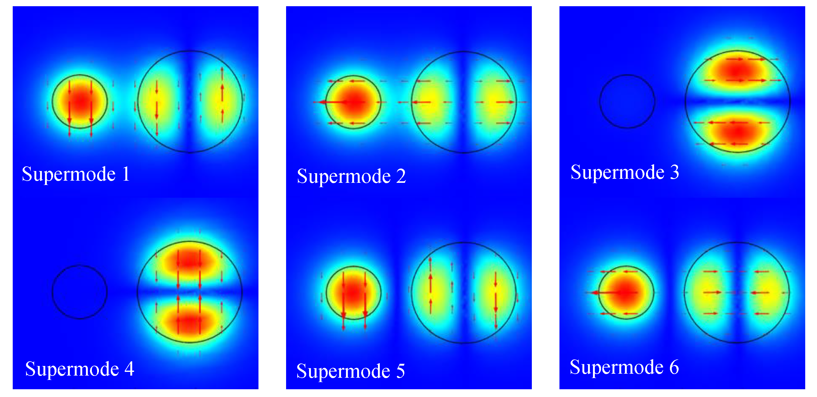
3.1. Supermodes for the MSC Structure

Firstly, we utilized the COMSOL software to obtain the supermodes of the MSC. Figure 2 shows the modal distributions of the six supermodes supported by an MSC structure obtained using COMSOL, whose parameters are set to be fiber core radius a₁ = 4.493 μm, a₂ = 8.56 μm, gap size d = 5 μm, cladding radius d_clad = 62.5 μm, cladding index n_cl = 1.444, core index n₁ = n₂ = 1.449, operating wavelength λ = 1.55 μm. The propagation constants of the supermodes decrease from supermode 1 to supermode 6, three of which correspond to the p-modes group (HE_11p-1, HE_21p-2, TM_01-2 modes). The remaining three supermodes correspond to the s-modes group (HE_11s-1, TE_01-2, HE_21s-2 modes) [29]. Now the question is which modes correspond to the p-modes group or s-modes group.

In order to answer this question, we calculated the modal distributions of the supermodes supported by the MSC. Based on the analysis in Section 2, the mode field of the supermode ψ_s(x, y) can be expressed as the linear combination of the mode field supported by the individual fiber waveguide that formed the MSC, denoted as

$$\left[\begin{array}{c}{\psi }_{s1}(x,y)\\ {\psi }_{s2}(x,y)\\ {\psi }_{s3}(x,y)\end{array}\right]={[\begin{array}{ccc}{\mathrm{v}}_1& {\mathrm{v}}_2& {\mathrm{v}}_3\end{array}]}^T\left[\begin{array}{c}{\psi }_1(x,y)\\ {\psi }_2(x,y)\\ {\psi }_3(x,y)\end{array}\right],$$

(22)

where ψ_sm(x, y) (m = 1, 2, 3) is the modal spatial distribution of the m-th supermode supported by the MSC structure, v_m is the corresponding eigenvector shown in Equation (9), and ψ_m(x, y) are the modal spatial distributions of the HE_11p-1, HE_21p-2, TM_01-2 modes, which can be described with accurate analytical expressions [18]. Simulation results are shown in Figure 3.

By comparing Figure 2 and Figure 3, we can observe that the supermodes 2, 4, 6 in Figure 2 are the supermodes corresponding to the p-modes group (HE_11p-1, HE_21p-2, TM_01-2 modes) and the supermodes 1, 3, 5 in Figure 2 are the supermodes corresponding to the s-modes group (HE_11s-1, TE_01-2, HE_21s-2 modes).

When considering the symmetry, the analysis here can be simplified. In fact, the p-modes (HE_11p-1, HE_21p-2, TM_01-2 modes) are mirror symmetric about the line connecting the two core center points, while the s-modes (HE_11s-1, TE_01-2, HE_21s-2 modes) are mirror antisymmetric. Therefore, the supermodes corresponding to the p-modes group and s-modes group should also be mirror symmetric and antisymmetric, respectively, as shown in Figure 2.

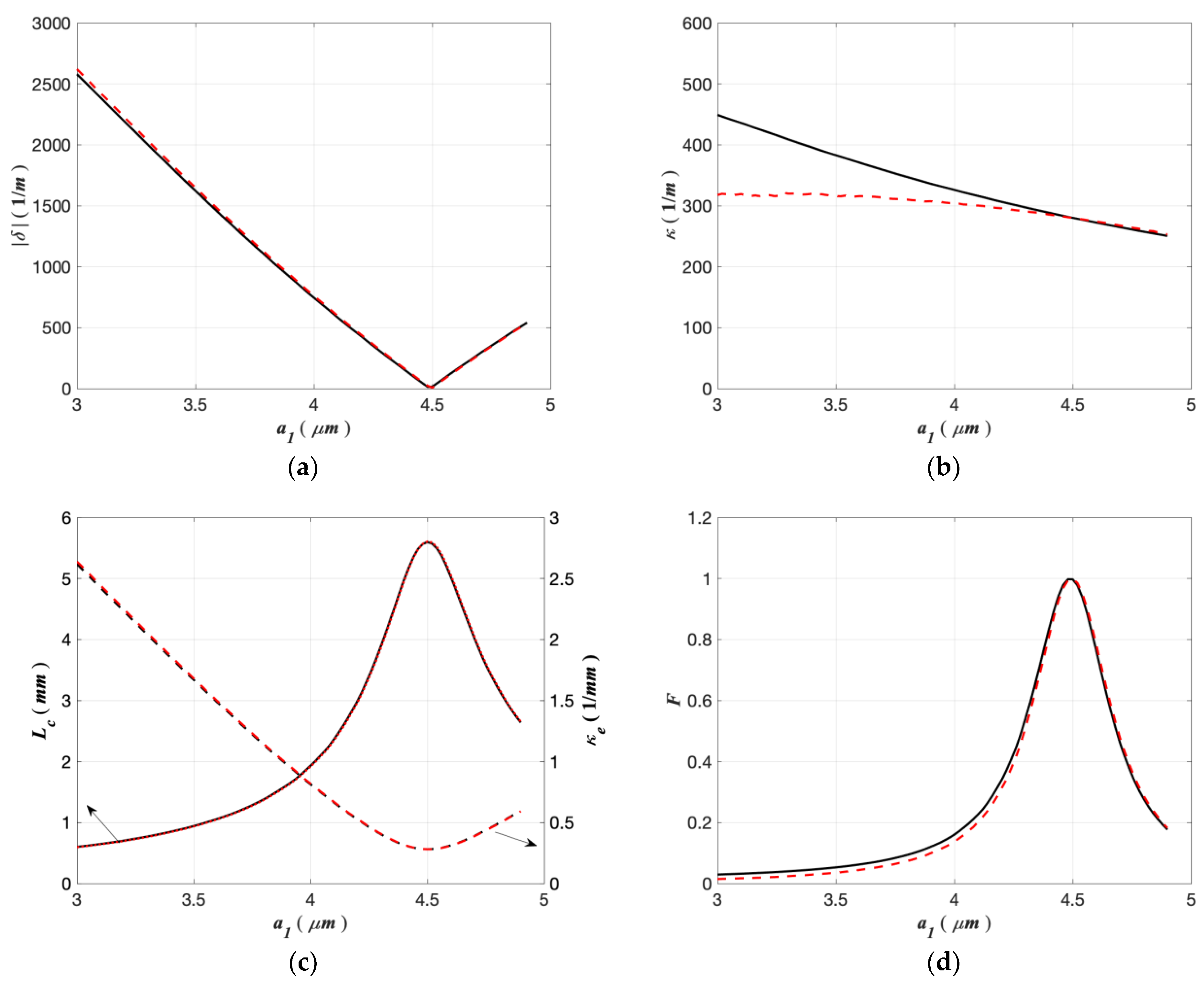
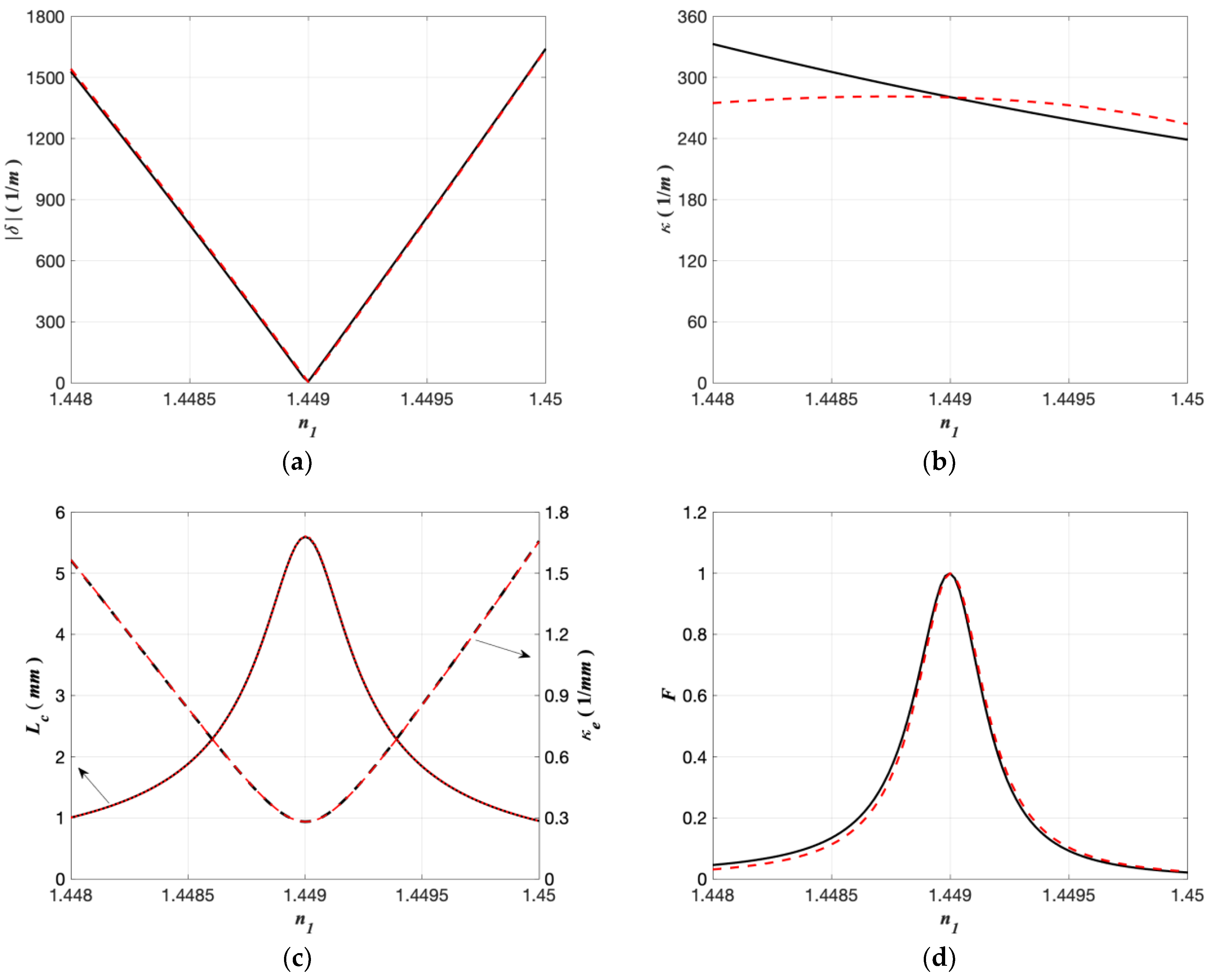
3.2. Calculation of the Characteristic Parameters of the MSC

In this section, simulations were carried out to verify the feasibility and accuracy of the supermode theory under different parameters of the MSC structure. The characteristic parameters of the MSC, including the difference of the propagation constants between the modes |δ|, coupling coefficient κ, effective coupling coefficient κ_e, coupling length L_c and maximum power-coupling efficiency F, were calculated using both the supermode theory and the traditional CMT under different parameters of the MSC structure, including gap size d, core radius a₁, and core index n₁.

Figure 4 shows the characteristic parameters of the MSC calculated using the two methods under different gap sizes. The red lines are obtained by the supermode theory, and the black lines are obtained by the traditional CMT. Parameters of the MSC structure are the same as those in Figure 2 except for the gap size.

As seen from Figure 4a,d, when the gap size between the two cores of the MSC is smaller than ~3.5 μm, there is a notable calculation error for the differences of the propagation constants |δ| and the maximum power-coupling efficiency F calculated using the two methods. This is due to the fact that the two cores are so close that strong coupling occurs between the modes. Therefore, there is some error when we represent the supermodes as linear combinations of the individual modes supported by the single fiber waveguides as in Equation (16). However, when the gap size is greater than ~3.5 μm, |δ| and F calculated using the two methods fit to each other quite well. In fact, for a practical MSC, normally the gap size between the two cores is greater than 4 μm.

As seen from Figure 4b, the calculation results for the coupling coefficient κ using the two methods match well with each other. Furthermore, the amplitude of the coupling coefficient κ is much greater than δ. Therefore, the effective coupling coefficient κ_e, which is defined as the square root of (δ² + κ²), is mainly determined by the value of κ. As a result, the effective coupling coefficients κ_e and corresponding coupling lengths L_c calculated by the two methods match well with each other, as seen from Figure 4c.

In Figure 4, the maximum power-coupling efficiency F is almost always 1 when the gap size increases from 0 to 15 μm. This is because the parameters of core 1 and core 2 are designed properly to ensure the HE_11p-1 mode and HE_21p-2/TM_01-2 mode are well phase-matched, i.e., the propagation constants of the three modes are almost the same (β₁ ≈ β₂). In other words, the MSC works at the phase matching point. This is also the reason why the amplitude of the coupling coefficient κ is much greater than δ.

However, for a practical MSC composed of an SMF and an FMF, it is difficult to ensure all parameters of the two fibers are so accurate. The core radius and index may be different from the designed value. Therefore, it is necessary to analyze the mode coupling characteristic under non-ideal conditions.

Figure 5 shows the characteristic parameters of the MSC calculated using the two methods under different core radiuses a₁. The red lines are obtained by the supermode theory, and the black lines are obtained by the traditional CMT. The other structure parameters of the MSC used here are the same as those in Figure 2. It should be pointed out that the core radius a₁ is limited to 4.9 μm in order to ensure the fiber core 1 only supports the fundamental mode.

As seen from Figure 5a,b, the differences of the propagation constants |δ| calculated using the two methods match well with each other when the core radius a₁ varies from 3 μm to 4.9 μm, while there is a notable calculation error for the coupling coefficient κ when a₁ is smaller than ~4.2 μm, which is different from the results in Figure 4. This is also due to the error when we represent the supermodes as linear combinations of the individual modes supported by the single fiber waveguides, as shown in Equation (16). When a₁ deviates from the phase matching point (a₁ ≈ 4.493 μm), the error between the modal distributions of the supermodes and the linear combinations of the individual modes increases. The coupling coefficient κ is determined by the overlap integral of the modal distributions in the CMT, as shown in Equation (3). Therefore, when a₁ deviates from the phase matching point, the error between the coupling coefficients calculated using the two methods increases.

As seen from Figure 5c, the effective coupling coefficients κ_e and corresponding coupling lengths L_c calculated by the two methods match well with each other when a₁ varies from 3 to 4.9 μm. This is because |δ| becomes significantly greater than κ when a₁ deviates from the phase matching point, thus κ_e and L_c are mainly determined by the value of |δ|.

As seen from Figure 5d, the maximum power-coupling efficiency F decreases when the core radius a₁ deviates from the phase matching point. F calculated using the supermode theory corresponds well with that obtained by the traditional CMT, besides slight errors when a₁ is smaller than ~4 μm. In fact, the maximum power-coupling efficiency F is less than ~17% when a₁ is smaller than ~4 μm, which should be avoided in the design and fabrication of the practical MSC.

Figure 6 shows the characteristic parameters of the MSC calculated using the two methods under different core indexes n₁. The other parameters are the same as those in Figure 2. Similarly to the above results in Figure 5, the differences of the propagation constants |δ| calculated using the two methods match well with each other when the core index n₁ varies from 1.448 to 1.45, while there are obvious differences for the coupling coefficient κ when n₁ deviates from the phase matching point (n₁ ≈ 1.449), as seen in Figure 6a,b. The reason for the calculation error for the coupling coefficient is the same with that in Figure 5. Furthermore, |δ| is significantly larger than κ when n₁ deviates from the phase matching point. Therefore, the effective coupling coefficients κ_e and the coupling lengths L_c calculated by the two methods match well with each other, as shown in Figure 6c.

As illustrated in Figure 6d, the maximum power-coupling efficiency F calculated using the supermode theory also corresponds well with that obtained from the traditional CMT, besides slight errors when n₁ is smaller than 1.4486. Furthermore, the maximum power-coupling efficiency F is less than ~20% when n₁ is smaller than 1.4486, which should be avoided in the design and fabrication of the practical MSC.

According to the above simulations and analyses, the characteristic parameters of the MSC (including the difference of the propagation constants |δ|, coupling coefficient κ, the effective coupling coefficient κ_e, coupling length L_c and maximum power-coupling efficiency F) calculated using the supermode theory match well with those calculated using the traditional CMT near the phase matching point. Therefore, the supermode theory is shown to be valid and accurate for analysis of the MSC near the phase matching point. When the structure parameter of the MSC deviates from the phase matching point, the maximum power-coupling efficiency F decreases quickly, which should be avoided in the design and fabrication of the practical MSC.

It should be noted that, although the analysis and simulations here are based on the mode coupling between the fundamental modes of SMF 1 (i.e., HE_11p-1, HE_11s-1) and the second-order modes of the FMF (i.e., TE_01-2, HE_21p-2, HE_21s-2, TM_01-2), the supermode theory is also valid for other kinds of MSC [30].

Especially for the analysis of MSC composed of fibers with complex index profiles, in which there are no analytical expressions for the modal distribution of the modes supported by the individual fiber waveguides, the analysis and design of the MSC are complex and time-consuming when using the traditional CMT. In this case, the supermode theory proposed in this paper will be a better choice.

4. Conclusions

In this paper, the supermode theory was applied in the analysis of the MSC. All the characteristic parameters of the MSC are expressed using the propagation constants of the supermodes supported by the MSC structure, which can be obtained using the common finite element software COMSOL directly, avoiding the complex double integral in the traditional CMT. Simulation results showed that the characteristic parameters calculated using the supermode theory corresponded well with those calculated using the traditional CMT near the phase matching point of the MSC structure. Therefore, this work provides a fast and accurate method for the analysis of the MSC, which is helpful for the design, fabrication and applications of the MSC.

References

1. Richardson, D.J.; Fini, J.M.; Nelson, L.E. Space-division multiplexing in optical fibres. Nat. Photonics 2013, 7, 354–362. [Google Scholar] [CrossRef] [Green Version]
2. Li, G.; Bai, N.; Zhao, N.; Xia, C. Space-division multiplexing: The next frontier in optical communication. Adv. Opt. Photonics 2014, 6, 413–487. [Google Scholar] [CrossRef] [Green Version]
3. Ismaeel, R.; Lee, T.; Oduro, B.; Jung, Y.; Brambilla, G. All-fiber fused directional coupler for highly efficient spatial mode conversion. Opt. Express 2014, 22, 11610–11619. [Google Scholar] [CrossRef] [PubMed] [Green Version]
4. Chang, S.H.; Chung, H.S.; Ryf, R.; Fontaine, N.K.; Han, C.; Park, K.J.; Kim, K.; Lee, J.C.; Lee, J.H.; Kim, B.Y.; et al. Mode- and wavelength-division multiplexed transmission using all-fiber mode multiplexer based on mode selective couplers. Opt. Express 2015, 23, 7164–7172. [Google Scholar] [CrossRef] [Green Version]
5. Chang, S.H.; Moon, S.-R.; Chen, H.; Ryf, R.; Fontaine, N.K.; Park, K.J.; Kim, K.; Lee, J.K. All-fiber 6-mode multiplexers based on fiber mode selective couplers. Opt. Express 2017, 25, 5734–5741. [Google Scholar] [CrossRef]
6. Igarashi, K.; Wakayama, Y.; Soma, D.; Tsuritani, T.; Morita, I.; Park, K.J.; Ko, J.; Kim, B.Y. Low-loss and low-crosstalk all-fiber-based six-mode multiplexer and demultiplexer for mode-multiplexed QAM signals in C-band. In Proceedings of the Optical Fiber Communication Conference, San Diego, CA, USA, 13–15 March 2018. paper Th1K. 3. [Google Scholar]
7. Luo, Y.; Zhou, W.; Wang, L.; Wang, A.; Wang, J. 16-QAM-carrying orbital angular momentum (OAM) mode-division multiplexing transmission using all-fiber fused mode selective coupler. In Proceedings of the Optical Fiber Communication Conference, San Diego, CA, USA, 13–15 March 2018. paper M4D. 2. [Google Scholar]
8. Wang, T.; Wang, F.; Shi, F.; Pang, F.; Huang, S.; Wang, T.; Zeng, X. Generation of femtosecond optical vortex beams in all-fiber mode-locked fiber laser using mode selective coupler. J. Lightwave Technol. 2017, 35, 2161–2166. [Google Scholar] [CrossRef] [Green Version]
9. Wang, T.; Shi, F.; Huang, Y.; Wen, J.; Luo, Z.; Pang, F.; Wang, T.; Zeng, X. High-order mode direct oscillation of few-mode fiber laser for high-quality cylindrical vector beams. Opt. Express 2018, 26, 11850–11858. [Google Scholar] [CrossRef]
10. Huang, Y.; Shi, F.; Wang, T.; Liu, X.; Zeng, X.; Pang, F.; Wang, T.; Zhou, P. High-order mode Yb-doped fiber lasers based on mode-selective couplers. Opt. Express 2018, 26, 19171–19181. [Google Scholar] [CrossRef]
11. Wan, H.; Wang, J.; Zhang, Z.; Cai, Y.; Sun, B.; Zhang, L. High efficiency mode-locked, cylindrical vector beam fiber laser based on a mode selective coupler. Opt. Express 2017, 25, 11444–11451. [Google Scholar] [CrossRef]
12. Shen, Y.; Ren, G.; Yang, Y.; Yao, S.; Xiao, S.; Jiang, Y.; Xu, Y.; Wu, Y.; Jin, W.; Jian, S. Generation of the tunable second-order optical vortex beams in narrow linewidth fiber laser. IEEE Photonics Technol. Lett. 2017, 29, 1659–1662. [Google Scholar] [CrossRef]
13. Zhang, Z.; Cai, Y.; Wang, J.; Wan, H.; Zhang, L. Switchable dual-wavelength cylindrical vector beam generation from a passively mode-locked fiber laser based on carbon nanotubes. IEEE J. Sel. Top. Quant. 2018, 24, 1100906. [Google Scholar] [CrossRef]
14. Wan, H.; Wang, J.; Zhang, Z.; Wang, J.; Ruan, S.; Zhang, L. Passively mode-locked Ytterbium-doped fiber laser with cylindrical vector beam generation based on mode selective coupler. J. Lightwave Technol. 2018, 36, 3403–3407. [Google Scholar] [CrossRef] [Green Version]
15. Cai, Y.; Wang, J.; Zhang, J.; Wan, H.; Zhang, Z.; Zhang, L. Generation of cylindrical vector beams in a mode-locked fiber laser using a mode-selective coupler. Chin. Opt. Lett. 2018, 16, 010602. [Google Scholar] [CrossRef]
16. Wang, J.; Wan, H.; Cao, H.; Cai, Y.; Sun, B.; Zhang, Z.; Zhang, L. A 1μm cylindrical vector beam fiber ring laser based on a mode selective coupler. IEEE Photonics Tech. L. 2018, 30, 765–768. [Google Scholar] [CrossRef] [Green Version]
17. Snyder, A.W. Coupled-Mode theory for optical fibers. J. Opt. Soc. Am. 1972, 62, 1267–1277. [Google Scholar] [CrossRef]
18. Okamoto, K. Fundamentals of Optical Waveguides; Academic: San Diego, CA, USA, 2005. [Google Scholar]
19. Agrawal, G.P. Applications of Nonlinear Fiber Optics; Academic: San Diego, CA, USA, 2001. [Google Scholar]
20. Zheng, Y.; Yao, J.; Zhang, L.; Wang, Y.; Wen, W.; Zhou, R.; Di, Z.; Jing, L. Supermode analysis in multi-core photonic crystal fiber laser. Proc. SPIE 2010, 7843, 784316. [Google Scholar]
21. Xia, C.; Bai, N.; Ozdur, I.; Zhou, X.; Li, G. Supermodes for optical transmission. Opt. Express 2011, 19, 16653–16664. [Google Scholar] [CrossRef]
22. Chan, F.Y.M.; Lau, A.P.T.; Tam, H.Y. Mode coupling dynamics and communication strategies for multi-core fiber systems. Opt. Express 2012, 20, 4548–4563. [Google Scholar] [CrossRef]
23. Ren, W.; Tan, Z. A study on the coupling coefficients for multi-core fibers. Optik 2016, 127, 3248–3252. [Google Scholar] [CrossRef]
24. Zhou, J. Analytical formulation of super-modes inside multi-core fibers with circularly distributed cores. Opt. Express 2014, 22, 673–688. [Google Scholar] [CrossRef]
25. Zhou, J. A non-orthogonal coupled mode theory for super-modes inside multi-core fibers. Opt. Express 2014, 22, 10815–10824. [Google Scholar] [CrossRef] [PubMed]
26. Szostkiewicz, L.; Napierala, M.; Ziolowicz, A.; Pytel, A.; Tenderenda, T.; Nasilowski, T. Cross talk analysis in multicore optical fibers by supermode theory. Opt. Lett. 2016, 41, 3759–3762. [Google Scholar] [CrossRef] [PubMed]
27. Bellanca, G.; Orlandi, P.; Bassi, P. Assessment of the orthogonal and non-orthogonal coupled-mode theory for parallel optical waveguide couplers. J. Opt. Soc. Am. A 2018, 35, 577–585. [Google Scholar] [CrossRef] [PubMed]
28. COMSOL Multiphysics Software. Available online: https://cn.comsol.com/ (accessed on 9 November 2021).
29. Lu, Y.; Huang, W.; Jian, S. Full vector complex coupled mode theory for tilted fiber gratings. Opt. Express 2010, 18, 713–726. [Google Scholar] [CrossRef] [PubMed]
30. Xu, Y.; Chen, S.; Wang, Z.; Sun, B.; Wan, H.; Zhang, Z. Cylindrical vector beam fiber laser with a symmetric two-mode fiber coupler. Photonics Res. 2019, 7, 1479–1484. [Google Scholar] [CrossRef]
Figure 1. Structure diagram of the MSC.
Photonics 09 00063 g001
Figure 2. The modal spatial distributions of the supermodes supported by an MSC structure, which are obtained using the commercial software COMSOL Multiphysics. The structural parameters of the MSC are set to be fiber core radius a1 = 4.493 μm, a2 = 8.56 μm, gap size d = 5 μm, cladding radius dclad = 62.5 μm, cladding index ncl = 1.444, core index n1 = n2 = 1.449, operating wavelength λ = 1.55 μm.
Photonics 09 00063 g002
Figure 3. (ac) are the modal spatial distributions of three supermodes supported by an MSC structure, which are composed of the p-modes group (HE11p-1, HE21p-2, TM01-2 modes) and obtained using the traditional CMT. The parameters of the MSC are the same as those in Figure 2.
Photonics 09 00063 g003
Figure 4. (a) The differences of the propagation constants |δ|, (b) coupling coefficient κ, (c) coupling length Lc, effective coupling coefficient κe, (d) maximum power-coupling efficiency F of the MSC under different gap sizes, which are calculated using the supermode theory (red lines) and the traditional CMT (black lines). The structure parameters of the MSC are the same as those used in Figure 2.
Photonics 09 00063 g004aPhotonics 09 00063 g004b
Figure 5. (a) The differences of the propagation constants |δ|, (b) coupling coefficient κ, (c) coupling length Lc, effective coupling coefficient κe, (d) maximum power-coupling efficiency F of the MSC under different core radiuses a1, which are calculated using the supermode theory (red lines) and the traditional CMT (black lines). The structure parameters of the MSC are the same as those used in Figure 2.
Photonics 09 00063 g005
Figure 6. (a) The differences of the propagation constants |δ|, (b) coupling coefficient κ, (c) coupling length Lc, effective coupling coefficient κe, (d) maximum power-coupling efficiency F of the MSC under different core indexes n1, which are calculated using the supermode theory (red lines) and the traditional CMT (black lines). The structure parameters of the MSC are the same as those used in Figure 2.
Photonics 09 00063 g006
Publisher’s Note: MDPI stays neutral with regard to jurisdictional claims in published maps and institutional affiliations.