Multilayer Photonic Spiking Neural Networks: Generalized Supervised Learning Algorithm and Network Optimization

Abstract

We propose a generalized supervised learning algorithm for multilayer photonic spiking neural networks (SNNs) by combining the spike-timing dependent plasticity (STDP) rule and the gradient descent mechanism. A vertical-cavity surface-emitting laser with an embedded saturable absorber (VCSEL-SA) is employed as a photonic leaky-integrate-and-fire (LIF) neuron. The temporal coding strategy is employed to transform information into the precise firing time. With the modified supervised learning algorithm, the trained multilayer photonic SNN successfully solves the XOR problem and performs well on the Iris and Wisconsin breast cancer datasets. This indicates that a generalized supervised learning algorithm is realized for multilayer photonic SNN. In addition, network optimization is performed by considering different network sizes.

1. Introduction

The brain exhibits great information processing capacity and superb energy efficiency. Experimental studies have shown that neurons in the brain form complex biological circuits that transmit information through rapid, spike-based signals [1]. It is widely accepted that rate coding and temporal coding are the two main spiking encoding approaches [2,3]. Rate coding is highly robust to peak-to-peak noise, and temporal coding takes full advantage of the temporal structure, with each spike having a high amount of information [4,5]. However, it is still controversial whether rate or temporal encoding dominates information encoding in the brain [6]. Motivated by spike-based neuromorphic systems, spiking neural network (SNN) was firstly proposed and demonstrated powerful computational capabilities [7]. SNN is more biologically plausible. Many advances of SNN have been reported in the fields of visual processing, speech recognition, and medical diagnostics [8,9,10,11,12].

An important problem in SNN is the differentiability of the spike trains that consist of Dirac functions. Compared to the multilayer artificial neural network (ANN), training a multilayer SNN is still in its infancy. The learning algorithm remains the most challenging problem for developing multilayer SNN. To solve the problem, some solutions have been proposed. For instance, the SpikeProp algorithm concentrated on approximating the neuronal membrane potential function to make it differentiable [13]. SpikeProp extends the traditional gradient descent-based (GDB) backpropagation algorithm to multilayer SNNs, making the output neurons fire precisely at the specified timing. Considering that spiking neurons may adopt multiple spikes to transmit information, a gradient descent-based multiple-spikes-learning algorithm was proposed and achieved high accuracy [14]. With binary activations, backpropagation has been adapted for a convolutional network [15]. In a similar manner, Bellec et al. successfully trained recurrent networks of spiking neurons with backpropagation through time using a piecewise linear surrogate derivative and found the result was comparable with conventional long short-term memory networks [16]. Neftci et al. further introduced a surrogate gradient in training SNN via interpreting SNNs as recurrent neural networks [17]. As recurrent connections are common in real neural networks, it will also be very interesting to consider recurrent networks in optical region. However, the spiking dynamic regime of the optical neuron should be clarified, as feedback connections may lead to quite complex dynamical phenomena such as chaos [18].

Recent attention has been attached on the spike-timing dependent plasticity (STDP) rule. The STDP rule is highly biologically interpretable [19,20]. In this rule, the synaptic weight is strengthened when the postsynaptic neuron fires shortly after the presynaptic neuron, and it is weakened when the postsynaptic neuron fires shortly before the presynaptic neuron [21]. The amount of change in synaptic weight depends exponentially on $t_{post}–t_{pre}$, where $t_{post}$ is the firing time of postsynaptic spike, and $t_{pre}$ denotes the firing time of the presynaptic spike. For example, the BP-STDP algorithm converted the backpropagation update rule into the STDP rule for the time subintervals in multilayer SNNs [22]. The BP-STDP model exhibited favorable performance in many datasets. In recurrent networks with spiking neuron, there are also relevant works to address discrepancy between the dynamical properties of synaptic plasticity and the requirements for gradient backpropagation [23,24].

In hardware, photonic SNNs have been employed to process many tasks [25,26]. The vertical-cavity surface-emitting lasers (VCSELs) have been employed as attractive photonic neurons in many photonic SNN models. For unsupervised learning, it was pointed out that photonic SNNs could achieve simple spike pattern learning and recognition tasks based on the photonic STDP [27]. Different functional processing tasks for photonic SNNs, including coincidence detection and pattern recognition, were also implemented experimentally [28]. Additionally, Deng et al. reported experimentally on the controllable propagation of spiking regimes between two interlinked VCSELs [29]. In addition, photonic spiking memory modules using single and mutually coupled VCSEL-neurons were demonstrated experimentally [30].

Note that, to solve some complex tasks, a multilayer photonic SNN may be required. For example, to solve the XOR problem, one approach was to build a multilayer photonic SNN, where a supervised learning algorithm modified the synaptic weights during training epochs [31]. Another approach was similar to a combinatorial logic circuit, where the XOR was decomposed into several basic logic operations, and different parts of the photonic SNN implemented different logic functions [32]. Feldmann et al. proposed an all-photonic SNN based on GST-based photonic neural elements, and the model performed well in the classification task of handwritten digits [33]. Han et al. proposed a supervised learning algorithm that combined the delay learning and the remote supervised method [34]. However, to the best of our knowledge, a generalized supervised learning algorithm for multilayer photonic SNNs still remains scarce.

In this study, we propose a generalized supervised learning algorithm for multilayer photonic SNNs by combing both the STDP rule and the gradient descent mechanism. The rest is organized as follows. Section 2 presents the multilayer photonic SNN model. The proposed model includes three parts: the neuron model based on VCSELs-SA, the architecture of the multilayer photonic SNN, and the generalized supervised learning algorithm for modifying synaptic weights among each layer. Section 3 describes the precoding process for the input patterns, and the parameters for training the network. Then, the trained network is employed to solve the XOR problem. In Section 4 and Section 5, we adopt the Iris dataset and Wisconsin breast cancer dataset to verify the generalization of the proposed multilayer photonic SNN. We also compare the proposed algorithm with other state-of-the-art algorithms. In addition, network optimization is performed by examining the impact of different sizes of input layer and hidden layer. In Section 6, a summary of the work is given.

2. Multilayer Photonic SNN Model

In this section, the spiking neuron model based on the VCSEL-SA is described. According to the presented rate equations, the firing processes of pre-synaptic neurons and post-synaptic neurons are illustrated. Then, the architecture of multilayer photonic SNN is presented. Finally, the loss function and the weight modification function based on the STDP rules and the gradient descent mechanism are presented.

2.1. Photonic Spiking Neuron Model

Here, the VCSEL-SA is adopted as a photonic spiking neuron. Here, the VCSEL-SA is adopted as a photonic spiking neuron, the schematic of which is presented in Figure 1a [35]. This model contains three dimensions, namely, the gain, the absorption, and the light intensity. Assuming that inputs only cause perturbations in the gain regime, which can be realized via selectively modulating the gain medium, this two-section laser can emulate the LIF neuron and generate spiking dynamics due to the different time scales of the three dimensions, and process information more than ten million times faster than a biological neuron [35]. The rate equations for the VCSEL-SA are presented as follows [36]:

$$\frac{\mathrm{d}{S}_{pre,post}}{dt}={\mathrm{\Gamma }}_a{g}_a(n_a-n_{0a})S_{pre,post}+{\mathrm{\Gamma }}_s{g}_s(n_s-n_{0s})S_{pre,post}-\frac{S_{pre,post}}{{\tau }_{ph}}+\beta B_r{n}_a^2$$

(1)

$$\frac{d{n}_a}{dt}=-{\mathrm{\Gamma }}_a{g}_a(n_a-n_{0a})(S-{\mathrm{\Phi }}_{pre}-{\mathrm{\Phi }}_{post})-\frac{n_a}{{\tau }_a}+\frac{I_a}{e{V}_a}$$

(2)

$$\frac{d{n}_s}{dt}=-{\mathrm{\Gamma }}_s{g}_s(n_s-n_{0s})S_{pre,post}-\frac{n_s}{{\tau }_s}+\frac{I_s}{e{V}_s}$$

(3)

$${\Phi }_{pre}=\frac{k_{ei}{\tau }_{ph}{\lambda }_{pre}{P}_{ei}({\tau }_i,\Delta \tau )}{hc{V}_a}$$

(4)

$${\Phi }_{post}={\displaystyle \sum _{i=1}^{\mathrm{N}}\frac{{\omega }_i{\lambda }_i{\tau }_{ph}{P}_i(t-T)}{hc{V}_a}}$$

(5)

$$P_{pre,post}(t)\approx \frac{hc{\eta }_c{\mathrm{\Gamma }}_a{S}_{pre,post}(t)V_a}{{\tau }_{ph}{\lambda }_{pre,post}}$$

(6)

The subscripts a and s stand for the gain and absorber regions, respectively. The subscripts pre and post represent PRE and POST neurons, respectively. S_pre,post represents the photonic density in the cavity. n_a (n_s) denotes the carrier density in the gain (absorber) region. The other parameters are defined in

Table 1. Some VCSEL-SA parameters used in the photonic SNN [35,36].

Description	Parameter and Value
Gain region cavity volume	$V_a$$=2.4\times {10}^{-18} {\mathrm{m}}^3$
SA region cavity volume	$V_s$$=2.4\times {10}^{-18}{ \mathrm{m}}^3$
Gain region confinement factor	${\Gamma }_a$ = 0.06
SA region confinement factor	${\Gamma }_s$ = 0.05
Gain region carrier lifetime	${\tau }_a$ = 1 ns
SA region carrier lifetime	${\tau }_s$ = 100 ps
Gain region differential gain/loss	$g_a$$=2.9\times {10}^{-12}{ \mathrm{m}}^3{\mathrm{s}}^{-1}$
SA region differential gain/loss	$g_s$$=14.5\times {10}^{-12} {\mathrm{m}}^3{\mathrm{s}}^{-1}$
Gain region transparency carrier density	$n_{0a}$$=1.1\times {10}^{24} {\mathrm{m}}^{-3}$
SA region transparency carrier density	$n_{0s}$$=0.89\times {10}^{24}{ \mathrm{m}}^{-3}$
Gain region input bias current	$I_a$ = 2 mA
SA region input bias current	$I_s$ = 0 mA
Lasing wavelength	$\lambda$ = 850 nm
Bimolecular recombination term	$B_r$$=10\times {10}^{-16} {\mathrm{m}}^3{\mathrm{s}}^{-1}$
Spontaneous emission coupling factor	$\beta$$=1\times {10}^{-4}$
Output power coupling coefficient	${\eta }_c$ = 0.4
Photon lifetime	${\tau }_{ph}$$=4.8\times {10}^{-12}$s
Velocity of light	$c = 3\times {10}^8{ \mathrm{ms}}^{-1}$
Planck constant	$h = 6.63\times {10}^{-34}$$\mathrm{J}$s

.

Equation (4) applies only to the PRE neurons, which represents the precoded stimuli. As a result, when calculating $n_a$ in PRE neurons by Equation (2), the expression $S-{\Phi }_{pre}-{\Phi }_{post}$ becomes $S-{\Phi }_{pre}$. The $k_{ei}$, ${\tau }_i$ and $\Delta$τ in Equation (4) correspond to precoded stimuli strength, center timing, and temporal duration. According to Equation (4) and Table 1, precoded stimuli strength is dimensionless, and we consider $k_{ei}$ = 2.9$\times {10}^3$, $\Delta$τ = 2 ns, $\Delta {\tau }_i$ = 0.05 ns. Equation (5) applies to the POST neurons, which characterizes the weighted summation. Similarly, $S-{\Phi }_{pre}-{\Phi }_{post}$ becomes $S-{\Phi }_{post}$ when calculating n_a in POST neurons by Equation (2). The simulation time window for neurons in each layer is [0, T].

To illustrate more details of the photonic spiking neuron, we consider the structure that one postsynaptic neuron is connected with some presynaptic neurons. In Figure 1b1, at the beginning, $n_a\left(t\right)$ keeps below the threshold (black dashed line), and the post-synaptic neuron does not fire. When the post-synaptic neuron gets spikes injected (green dashed lines), $n_a$(t) increases. Once the $n_a\left(t\right)$ exceeds the threshold, post-synaptic neuron fires, and the firing time is recorded as $t_o$. After that, $n_a\left(t\right)$ decreases rapidly and then gradually recovers. As depicted in Figure 1b2, during the training process, there may be spikes that arrive after the sample label ($t_N+d>t_{label}$), and these corresponding synaptic weights will not be modified.

2.2. Network of Photonic Spiking Neurons

The architecture of the proposed multilayer photonic SNN is depicted in Figure 2. The fully connected network consists of input, hidden, and output layers, labeled with I, H, and O, respectively. The number of neurons in each layer is denoted by $N_i$, $N_h$, and $N_o$, where $N_o$ = 1. Here, the input neurons belong to the PRE neurons, and the rate equations are Equations (1)–(4) and (6). Additionally, the hidden neurons and output neurons belong to the POST neurons, since they process the spikes from the previous layer. The rate equations are similar to those in Equations (1)–(3), (5) and (6). However, note that, for the hidden neurons, in Equation (5), the terms N and ${\omega }_i$ should be replaced by $N_i$ and ${\omega }_{ih}$, respectively. For the output neuron, in Equation (5), the subscript I, the term N and ${\omega }_i$ should be replaced by j, $N_h$, and ${\omega }_{jo}$, respectively.

$${\Phi }_{post}={\displaystyle \sum _{i=1}^{N_i}\frac{{\omega }_{ih}{\lambda }_i{\tau }_{ph}{P}_i(t-T)}{hc{V}_a}}$$

(7)

$${\Phi }_{post}={\displaystyle \sum _{\mathrm{j}=1}^{N_h}\frac{{\omega }_{jo}{\lambda }_j{\tau }_{ph}{P}_j(t-T)}{hc{V}_a}}$$

(8)

As shown in Figure 2b, external stimuli are firstly pre-processed into the precoded stimulus signals, and the center timing of the rectangular pulse is recorded as $t_{in}$. The $d_{in}$ indicates the afferent delay of the precoded rectangular pulses to the input neurons. Each input neuron has only one afferent connection. For simplicity, we suppose that the neurons in the input layer can emit up to one spike. The spiking time of input neurons is recorded as $t_i$. If there is no spike output for a neuron, the spiking time is recorded as T, which means the ending of the simulation time window.

The ${\omega }_{ih}$ ($d_{ih}$) represents the synaptic weight (delay) between an input neuron and a hidden neuron. The firing time of spike generated by the hidden neuron is recorded as $t_h$. It is possible for neurons in a hidden layer or output layer to generate more than one spike at once. We adopt the first-to-spike strategy [37]. Namely, the firing time of the first spike is utilized to denote the result. The $t_{label}$ denotes the labels of corresponding input patterns.

For a possible hardware implementation, as shown in Figure 3, the input data are firstly pre-encoded into pulses with a pulse pattern generator (PPG) and then modulated to optical carriers from laser diodes (LDs) via MZM modulator array. The output from an input layer neuron is firstly amplified by a semiconductor optical amplifier (SOA) and then split into an $N_h$ beam for a full connection to the hidden layer neurons. A similar approach can be used for more hidden layer connections. The coupling strength from the input to the hidden neurons and from the hidden to the output can be modified by the variable optical attenuators (VOA), according to the algorithms implemented in the electronic controller. Delay lines are arranged for delay compensation of different optical path. Because VCSEL is easy for large-scale integration, the proposed SNN can be practically scaled in the hardware architecture [31].

2.3. The Synaptic Weight Modification Function by Combing the STDP and the Gradient Descent

We use the mean squared error (MSE) as the loss function in a training epoch. MSE is calculated as the squared loss divided by the number of samples as follows:

$$MSE=\frac{1}{M}{\displaystyle \sum _{m=1}^M{(\overline{t_{o_m}-t_{labe{l}_m}})}^2}$$

(9)

where M represents the number of samples in the training set or test set, and $\overline{t_o-t_{label}}=\frac{t_o-t_{label}}{1 \mathrm{ns}}$ means normalization of the time difference. For single input pattern, Equation (9) becomes ${(\overline{t_o-t_{label}})}^2$, and we can obtain the derivative of the term to $t_o$

$$\frac{\partial {(\overline{t_o-t_{label}})}^2}{\partial t_o}=2 \overline{t_o-t_{label}}$$

(10)

Hence, by combing the STDP rule and the gradient descent rule, the functions for synaptic weight modifications $\Delta \omega$ become:

$$\Delta {\omega }_{oh}=-\eta (\overline{t_o-t_{label}})\times \Delta {\omega }_{STDP}\left[t_o-(t_h+d_{ho})\right]$$

(11)

$$\Delta {\omega }_{hi}=\eta (\overline{t_o-t_{label}})\times \Delta {\omega }_{STDP}\left[t_h-(t_i+d_{ih})\right]$$

(12)

Finally, the synaptic weights in each layer are updated as follows:

$$\omega (x+1)=\omega (x)+\Delta \omega$$

(13)

Equation (11) applies to synaptic weights modification between the hidden and output layers, and Equation (12) applies to synaptic weights modification between the input and hidden layers. The $\eta$ indicates learning rate; during the training process, $\omega$ is strengthened or weakened, and we assume that $\omega$ keeps non-negative because $\omega$ indicates the connection strength between VCSELs-SA.

3. The XOR Benchmark

The XOR problem is a classic linearly inseparable problem. Minsky et al. first demonstrated that the problem could not be solved by single layer neural network [38]. The input patterns of XOR problem are binary symbols “0” and “1”. The firing time of the output neuron represents the prediction of the network. The input patterns 00, 01, 10, and 11 correspond to 8.5 ns, 10.5 ns, 10.5 ns, and 8.5 ns, respectively.

3.1. Precoding

To encode real valued features into a temporal pattern, we employ a set of Gaussian functions [13]. The m denotes the number of Gaussian function, which means each feature is assigned to m input neurons. The center of the Gaussian functions $\mu$ is given by

$${\mu }_i=I_{min}+\frac{2i-3}{2}\cdot \frac{I_{max}-I_{min}}{m-2},i=1,2,\cdots ,m$$

(14)

where m = 4, $I_{min}$ = −0.1, and $I_{max}$ = 1.25. The variance of the Gaussian functions is the same and is calculated as

$$\sigma =\frac{1}{\beta }\cdot \frac{I_{max}-I_{min}}{m-2}$$

(15)

where $\beta$ is set to 1. As depicted in Figure 4, the horizontal coordinate represents real valued features, binary symbols “0” and “1”, for example. The vertical coordinate ranges from 0 to 3 ns. Then, each precise vertical coordinate is rounded to its nearest time step, which is set as 0.05 ns. The quantified result is recorded as $t_{\mathrm{in}}$ (as presented in Figure 2b). Especially, if $t_{in}$ = 0 ns, the corresponding input neuron will not be stimulated; hence, it will fire at T. Moreover, for a given feature in a dataset, the maximum $I_{max}$ and minimum $I_{\min }$ are known. According to Equations (14) and (15), parameters m and $\beta$ can affect the precoding result. The simulation results suggest that proper parameters m and $\beta$ are friendly to the network performance.

3.2. Technical Details

The architecture of the multilayer photonic SNN and learning algorithm applied are described in Section 2, where $N_i$ = 8, $N_h$ = 6, and $N_o$ = 1. The simulation time window is 0–12 ns, and T is 12 ns. The learning rate $\eta$ is set as 2.2$\times {10}^{-2}$. In simulation, the sample label 8.5 ns is expanded into the interval (8.3 ns, 8.7 ns), and label 10.5 ns is expanded into the interval (10.3 ns, 10.7 ns). If the prediction of output neuron falls inside the corresponding interval, it is considered right. Synaptic weights in the network are randomly initialized. After each training epoch, the training result and MSE (Equation (9)) are recorded. The training process converges when all the predicted results fall into the corresponding interval.

3.3. Analysis of Learning Process

Figure 5a illustrates the firing time of output neuron in training. At the beginning, the network cannot output right predictions. With the synaptic weights modified, the network correctly predicts for the input patterns “01” (orange) and “10” (yellow) at about the 20th epoch. At about the 50th epoch, the network gradually achieves correct predictions of the input patterns “11” (purple) and “00” (blue). Finally, the learning process ends at the 60th epoch. Figure 5b presents the relationship between loss function MSE and training epoch, where the vertical axis takes logarithmic coordinates. It can be seen that the value of MSE drops and eventually converges at the 60th epoch. Figure 6 further presents the normalized synaptic weights $\overline{\omega }$ over training epochs. Here, $\overline{\omega }$ is calculated as $\frac{\omega -{\omega }_{\min }}{{\omega }_{\max }-{\omega }_{\min }}$, where ${\omega }_{max}$ (${\omega }_{min}$) is the maximum (minimum) of the synaptic weights in training. The numbers indicate neuron index in different layers. As depicted in Figure 6a1,a2, the initial synaptic weights are random. Compared with Figure 6a1,a2,c1,c2, during the training process, many synaptic weights have been modified.

After the training process, we further adopt the trained weight to perform inference task. As shown in Figure 7, for 00, 11, the POST fires at 8.5ns. For 01 and 10, the POST fires at 10.5ns. That is to say, with these trained weights, the XOR task can be successfully solved.

4. The Iris Benchmark

Iris flower dataset contains three classes of Iris flowers, Iris setosa, Iris versicolor, and Iris virginica [39]. Each of the three species consists of 50 samples. There are four features measured from each sample: the length and the width of the sepals, and the length and the width of petals. For classification, Iris setosa is linearly separable from the other two, whereas Iris versicolor and Iris virginica are not linearly separable from each other.

4.1. Technical Details

The 150 samples are randomly divided into two sets, and 100 of them are used for training and the rest are used for testing. Sample labels of Iris setosa, Iris versicolor, and Iris virginica are set as 8.5 ns, 10 ns, and 11.5 ns, respectively. As for precoding process, $I_{max}$ and $I_{min}$ are the maximum and minimum value of the sample features, so there are four pairs of $I_{\max }$ and $I_{\min }$. We consider the network size as $N_i$ = 24, $N_h$= 20, and $N_o$= 1. The simulation time window is 0–14 ns, and T is 14 ns. The learning rate is $\eta$ = 5.5$\times {10}^{-4}$. Moreover, a strategy named early stopping is introduced during training in the Iris dataset and the Wisconsin breast cancer dataset [40]. Early stopping is widely adopted in fully connected networks to avoid overfitting.

4.2. Classifying the Iris Dataset

Predictions of the network on training set are depicted in Figure 8. Input patterns in the training set are randomized and predictions are re-sorted according to the true labels. The firing time of output neuron $t_o$ (orange circle) means the predicted label, and the blue circle means true label. The dotted lines at 9 ns and 10.85 ns are the boundaries of the true labels. Three time intervals [8 ns, 9 ns], [9 ns, 10.85 ns], and [10.85 ns, 12 ns] correspond to Iris setosa, Iris versicolor, and Iris virginica, respectively. As can be seen in Figure 8, all the Iris setosa samples are correctly predicted. As labeled by the shading parts in Figure 8, two samples of Iris versicolor and one sample of Iris virginica are not correctly predicted. The training accuracy is about 97%. That is to say, the predicting performance of the Iris setosa samples is better than those of the other two classes.

Figure 9a shows the normalized confusion matrix for test set of Iris dataset. The value in matrix indicates the average test accuracy. The vertical axis indicates the true label, and the horizontal axis indicates the predicted label. Numbers 1, 2, and 3 in the coordinate axes correspond to the three classes of Iris flowers: Iris setosa, Iris versicolor, and Iris virginica. It can be seen that all the samples that belong to class 1 are predicted correctly. For class 2 (3), 91.7% (95.2%) of the samples are correctly predicted.

Next, we further consider the effect of network size on the network performance. Figure 10a presents the MSE as a function of epochs for four different sizes of hidden layer, which are denoted in different colors. Obviously, the MSE values decrease to a low level and converge for all the cases of network sizes. Namely, the training convergence can be achieved for all the considered network sizes. Figure 10b further presents the MSE when the learning process converges. It can be found that, for Iris benchmark, the proper size of hidden layer (above 20) contributes to the performance of the network.

5. The Wisconsin Breast Cancer Benchmark

The Wisconsin breast cancer dataset contains two classes: benign sample and malignant sample [41]. Considering the original dataset contains 16 samples with missing data, we adopt the dataset containing the rest 683 samples (444 benign samples and 239 malignant samples). Each sample consists of nine features, and we choose four features in the dataset (Uniformity Of Cell Size, Uniformity Of Cell Shape, Marginal Adhesion, and Single Epithelial Cell Size) as input patterns. The 683 samples were randomly divided: 400 of the samples were used for training, and the rest were used for testing. We set labels of “benign” and “malignant” to 8.5 ns and 11 ns, respectively. For the network size, we set $N_i$ = 28, $N_h$ = 20, and $N_o$ = 1. The simulation time window is 0–14 ns, and T is 14 ns. The learning rate is $\eta$ = 5.5$\times {10}^{-4}$.

5.1. Classifying the Wisconsin Breast Cancer Dataset Dataset

The spiking time of output neuron in the training process is depicted in Figure 11. Two different situations in the training process are illustrated. For most input patterns, as presented in Figure 11a, after some training epochs, the predicted labels come close to the true label, whereas for some input patterns, as shown in Figure 11b, the training process converges slowly. The predicted labels come close to the true label after several hundred training epochs.

Predictions of the trained network on test set are depicted in Figure 12. The time ranges [8 ns, 9.3 ns] and [9.3 ns, 12 ns] correspond to the label “benign” and label “malignant”. We can see from Figure 12 that the prediction performance of the malignant is better than that of the benign. To further quantify the prediction performance, we present the confusion matrix for the average test accuracy of breast cancer dataset in Figure 9b. Numbers 2 and 4 in the coordinate axes correspond to “benign” and “malignant”. It can be seen that 94.6% of the samples belonging to class 2 (benign) are correctly classified, whereas 98.9% of the samples belonging to class 4 (malignant) are correctly predicted.

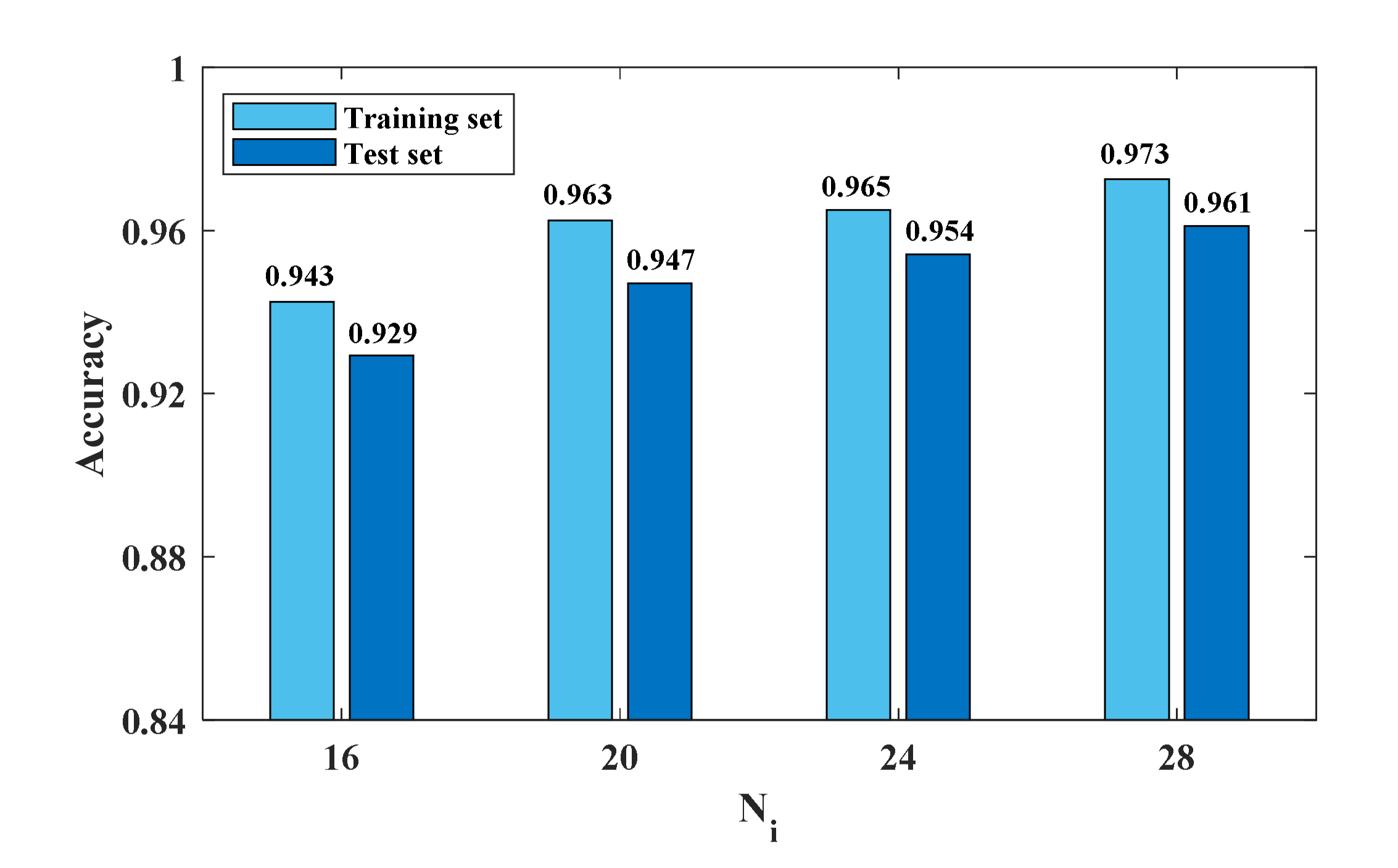
5.2. Learning with the Various Sizes of Input Layer

As can be seen in precoding, a larger input layer implies that the spiking times of the input neurons are presented in more dispersed distribution, and this may improve the network performance. Figure 13 shows the accuracy for multilayer photonic SNN with different sizes of input layer. These networks adopt the same dataset partitioning and the same size of hidden layer to ensure a fair comparison. It can be seen that both training and test accuracies are improved, as the $N_i$ grows from 16 to 28. Therefore, properly increasing the input layer size contributes to the network performance.

6. Discussion

Then, we tried to estimate the energy consumed in our network on performing Iris or Wisconsin breast cancer datasets. The energy efficiency in an SNN can be reasonably simplified by calculating the energy consumed by a spike activity and the number of spikes generated during processing [42]. Therefore, we can assume that the energy consumed by a spiking activity in a VCSEL-SA-based neuron is E which could be estimated as $\mathrm{FWHM}\times {\mathrm{P}}_{\max }$, where FWHM is the full width at half maximum of an optical pulse (which is about 0.025 ns), and ${\mathrm{P}}_{\max }$ is the peak power (about 6 mW in simulation, the actual pulse width will be much larger due to device limitations). The spike numbers generated in the inference task of the Iris dataset and breast cancer dataset are about 35 and 39, respectively. Hence, the total power consumed for the two datasets can be calculated as:

Iris dataset: $\left(0.025\times {10}^{-9}\right)\times \left(6\times {10}^{-3}\right)\times 35=5.25 \mathrm{pJ}$

Wisconsin breast cancer dataset: $\left(0.025\times {10}^{-9}\right)\times \left(6\times {10}^{-3}\right)\times 35=5.85 \mathrm{pJ}$

However, more reliable calculation should be based on hardware. Unfortunately, VCSEL-SA is not commercially available.

Table 2. The comparison of performance for proposed algorithm with the state-of-the-art techniques.

Algorithm	Network Architecture	Convergence Epoch	Accuracy (%)
			Training Set	Test Set
Iris dataset
SpikeProp [13]	50-10-3	1000	97.4 ± 0.1	96.1 ± 0.1
SWAT [43]	16-208-3	500	95.5 ± 0.6	95.3 ± 3.6
SRESN (online) [44]	6-11	102	92.7 ± 4.2	93.0 ± 5.7
DEPT-ESNN [45]	—	—	99.3 ± 0.2	89.3 ± 3.4
SpiFoG [46]	—	299	97.4 ± 0.9	97.2 ± 2.1
This work	24-20-1	440	96.8 ± 0.8	96.0 ± 1.3
Wisconsin breast cancer dataset
SpikeProp	64-15-2	1500	97.6 ± 0.2	97.0 ± 0.6
SWAT	9-117-2	500	96.2 ± 0.4	96.7 ± 2.3
SRESN (online)	5-8	306	93.9 ± 1.8	94.0 ± 2.6
OSNN [47]	54-22-2	—	91.1 ± 2.0	90.4 ± 1.8
SpiFoG	—	896	98.3 ± 0.3	97.9 ± 0.1
This work	28-20-1	300	97.3 ± 0.5	96.1 ± 0.8

shows a comparison of network architecture, training epoch and mean accuracy with state-of-the-art techniques. It can be seen that, for the two benchmarks, at most, one hidden layer is required to achieve high performance. However, for more complex datasets, a deeper network may be required. For the Iris dataset, DEPT-ESNN shows 99.3% ± 0.2% accuracy (training set), and SpiFoG shows 97.2% ± 2.1% accuracy (test set). Our algorithm for multi-layer photonic SNN shows 96.0% ± 1.3% (test set), which is better than the majority of algorithms in Table 2. For the Wisconsin breast cancer dataset, SpiFoG shows 98.3% ± 0.3% accuracy (training set), and 97.9% ± 0.1% accuracy (test set). Our algorithm shows 97.3% ± 0.5% (training set). In the network architecture column, the number of network parameters can be calculated. For the SpikeProp, each synaptic connection consists of 16 delayed sub-connections. Hence, in order to learn the Iris dataset there are 16$\times$(50$\times$10 + 10$\times$3) = 8480 individual weights that need to be modified. For the SRESN (online), to learn the Iris dataset, there are 120 + 220 = 340 network parameters to be modified, whereas for the breast cancer dataset, the number becomes 270 + 432 = 702. For the OSNN, each synaptic connection also consists of 16 delayed sub-connections.

For the Iris dataset, the parameters needed in our algorithm (500) are much fewer than those for SpikeProp (8480) and SWAT (624). For the breast cancer dataset, the parameters needed in our algorithm are also fewer than for SpikeProp, SRESN (online), and OSNN. By taking the training epoch and network architecture into account, for the multi-layer photonic SNN, our algorithm offers competitive performance for the conventional SNN algorithms.

We also try to apply the proposed algorithm to the MNIST dataset, which is larger and more complex. Considering that the VCSLE-SA-based neuron model is computationally complex, and the training process is time-consuming, we use a relatively simple LIF neuron model and select 1000 samples from MNIST dataset for training. We first apply Principal Component Analysis to reduce the dimension of the sample to 20 and use the precoding method described in Chapter 3. In this way, the input is pre-coded into a 200-dimension vector. Here, we consider two networks with one hidden layer and two hidden layers, the network size of which are $200\times 30\times 1$ and $200\times 30\times 25\times 1$, respectively. However, the training accuracy can only reach to 90%, which is most probably because the adjustment of weight is not based on strict gradient calculation, and the network will be greatly affected by accumulated errors as the depth of the network increases.

7. Conclusions

In this study, we propose a generalized supervised learning algorithm to train a multilayer photonic SNN. To achieve high energy efficiency, VCSELs-SA are employed as LIF neurons in the network considering the ultra-low energy consumption [48]. A modified learning algorithm combining the STDP rule and the gradient descent mechanisms is applied. Temporal coding is employed in the network. A precoding process is adopted for input patterns, and it translates the real valued features of samples into signals that fit photonic neurons. The First-to-Spike strategy is introduced, so that there is at most one spike carrying information in each synaptic connection.

We apply the proposed algorithm to train multilayer photonic SNN, and the XOR problem is solved successfully. In addition, two relatively small datasets including Iris datasets and the Wisconsin breast cancer dataset are also adopted to demonstrate the performance of our proposed algorithm. Simulation results clarify that the proposed algorithm performs well in these datasets, which shows the generalization of the algorithm. However, as the considered datasets are relatively simple, it cannot be concluded that this approach is applicable to all practical situations. As a future attempt, by further optimizing and reducing the running time of the optical SNN model, it is also interesting and meaningful to consider larger datasets such as MNIST or CIFAR-10. The superiority of the algorithm will be more significant when the network architecture and the training epochs are taken into account. The proposed algorithm for photonic SNN also has the advantages of ultrafast processing rate. Once the input signals are injected into the photonic SNN, the output classification results can be achieved within several tens of nanoseconds. With more optimization of the various synaptic connection delays, the processing time may be reduced further.

References

1. Hodgkin, A.L.; Huxley, A.F. A quantitative description of membrane current and its application to conduction and excitation in nerve. J. Physiol. 1952, 117, 500–544. [Google Scholar] [CrossRef]
2. Dayan, P.; Abbott, L.F. Theoretical Neuroscience: Computational and Mathematical Modeling of Neural Systems; MIT Press: Cambridge, MA, USA, 2001. [Google Scholar]
3. Gerstner, W.; Kistler, W.M.; Naud, R.; Paninski, L. Neuronal Dynamics: From Single Neurons to Networks and Models of Cognition; Cambridge University Press: Cambridge, UK, 2014. [Google Scholar]
4. London, M.; Roth, A.; Beeren, L.; Hausser, M.; Latham, P. Sensitivity to perturbations implies high noise and suggests rate coding in cortex. Nature 2010, 466, 123–127. [Google Scholar] [CrossRef] [Green Version]
5. Hopfield, J.J. Pattern recognition computation using action potential timing for stimulus representation. Nature 1995, 376, 33–36. [Google Scholar] [CrossRef]
6. Masuda, N.; Aihara, K. Bridging rate coding and temporal spike coding by effect of noise. Phys. Rev. Lett. 2002, 88, 248101. [Google Scholar] [CrossRef]
7. Maass, W. Networks of spiking neurons: The third generation of neural network models. Neural Netw. 1997, 10, 1659–1671. [Google Scholar] [CrossRef]
8. Escobar, M.J.; Masson, G.S.; Vieville, T.; Kornprobst, P. Action recognition using a bio-inspired feedforward spiking network. Int. J. Comput. Vis. 2009, 82, 284–301. [Google Scholar] [CrossRef]
9. Wysoski, S.G.; Benuskova, L.; Kasabov, N. Evolving spiking neural networks for audiovisual information processing. Neural Netw. 2010, 23, 819–835. [Google Scholar] [CrossRef]
10. Tavanaei, A.; Maida, A. Bio-inspired multi-layer spiking neural network extracts discriminative features from speech signals. In Proceedings of the International Conference on Neural Information Processing, Guangzhou, China, 14–18 November 2017; pp. 899–908. [Google Scholar]
11. Ghosh-Dastidar, S.; Adeli, H. A new supervised learning algorithm for multiple spiking neural networks with application in epilepsy and seizure detection. Neural Netw. 2009, 22, 1419–1431. [Google Scholar] [CrossRef]
12. Kasabov, N.; Feigin, V.; Hou, Z.; Chen, Y.; Liang, L.; Krishnamurthi, R.; Othman, M.; Parmar, P. Evolving spiking neural networks for personalised modelling, classification and prediction of spatio-temporal patterns with a case study on stroke. Neurocomputing 2014, 134, 269–279. [Google Scholar] [CrossRef] [Green Version]
13. Bohte, S.M.; Kok, J.N.; Han, L.P. Error-backpropagation in temporally encoded networks of neurons. Neurocomputing 2000, 48, 17–37. [Google Scholar] [CrossRef] [Green Version]
14. Xu, Y.; Zeng, X.; Han, L.; Yang, J. A supervised multi-spike learning algorithm based on gradient descent for spiking neural networks. Neural Netw. 2013, 43, 99–113. [Google Scholar] [CrossRef]
15. Esser, S.K.; Merolla, P.A.; Arthur, J.V.; Cassidy, A.S.; Appuswamy, R.; Andreopoulos, A.; Berg, D.J.; McKinstry, J.L.; Melano, T.; Barch, D.R.; et al. Convolutional networks for fast, energy-efficient neuromorphic computing. Proc. Natl. Acad. Sci. USA 2016, 113, 11441–11446. [Google Scholar] [CrossRef] [Green Version]
16. Bellec, G.; Salaj, D.; Subramoney, A.; Legenstein, R.; Maass, W. Long short-term memory and learning-to-learn in networks of spiking neurons. In Proceedings of the Advances in Neural Information Processing Systems, Montréal, QC, Canada, 4–5 December 2018. [Google Scholar]
17. Neftci, E.O.; Mostafa, H.; Zenke, F. Surrogate gradient learning in spiking neural networks: Bringing the power of gradient-based optimization to spiking neural networks. IEEE Signal Process. Mag. 2019, 36, 51–63. [Google Scholar]
18. Zhao, A.; Jiang, N.; Zhang, Y.; Peng, J.; Liu, S.; Qiu, K.; Deng, M.; Zhang, Q. Semiconductor Laser-Based Multi-Channel Wideband Chaos Generation Using Optoelectronic Hybrid Feedback and Parallel Filtering. J. Lightwave Technol. 2022, 40, 751–761. [Google Scholar] [CrossRef]
19. Caporale, N.; Dan, Y. Spike timing-dependent plasticity: A hebbian learning rule. Annu. Rev. Neurosci. 2008, 31, 25–46. [Google Scholar] [CrossRef] [Green Version]
20. Markram, H.; Gerstner, W.; Sjöström, P.J. Spike-timing-dependent plasticity: A comprehensive overview. Front. Synaptic Neurosci. 2012, 4, 2. [Google Scholar] [CrossRef] [Green Version]
21. Abbott, L.F.; Nelson, S.B. Synaptic plasticity: Taming the beast. Nat. Neurosci. 2000, 3, 1178–1183. [Google Scholar] [CrossRef]
22. Tavanaei, A.; Maida, A.S. BP-STDP: Approximating backpropagation using spike timing dependent plasticity. Neurocomputing 2017, 330, 39–47. [Google Scholar] [CrossRef] [Green Version]
23. Kaiser, J.; Mostafa, H.; Neftci, E. Synaptic plasticity dynamics for deep continuous local learning (DECOLLE). Front. Neurosci. 2020, 14, 424. [Google Scholar] [CrossRef]
24. Bellec, G.; Scherr, F.; Subramoney, A.; Hajek, E.; Salaj, D.; Legenstein, R.; Maass, W. A solution to the learning dilemma for recurrent networks of spiking neurons. Nat. Commun. 2020, 11, 3625. [Google Scholar] [CrossRef]
25. Pammi, V.A.; Alfaro-Bittner, K.; Clerc, M.G.; Barbay, S. Photonic computing with single and coupled spiking micropillar lasers. IEEE J. Sel. Top Quantum Electron. 2020, 26, 1500307. [Google Scholar] [CrossRef] [Green Version]
26. Xiang, S.; Ren, Z.; Zhang, Y.; Song, Z.; Hao, Y. All-optical neuromorphic XOR operation with inhibitory dynamics of a single photonic spiking neuron based on VCSEL-SA. Opt. Lett. 2020, 45, 1104–1107. [Google Scholar] [CrossRef]
27. Xiang, S.; Zhang, Y.; Gong, J.; Guo, X.; Lin, L.; Hao, Y. STDP-based unsupervised spike pattern learning in a photonic spiking neural network with VCSELs and VCSOAs. IEEE J. Sel. Top Quantum Electron. 2019, 25, 1700109. [Google Scholar] [CrossRef]
28. Robertson, J.; Matěj, H.; Julián, B.; Hurtado, A. Ultrafast optical integration and pattern classification for neuromorphic photonics based on spiking VCSEL neurons. Sci. Rep. 2020, 10, 6098. [Google Scholar] [CrossRef] [Green Version]
29. Deng, T.; Robertson, J.; Hurtado, A. Controlled propagation of spiking dynamics in vertical-cavity surface-emitting lasers: Towards neuromorphic photonic networks. IEEE J. Sel. Top Quantum Electron. 2017, 23, 1800408. [Google Scholar] [CrossRef] [Green Version]
30. Robertson, J.; Wade, E.; Kopp, Y.; Bueno, J.; Hurtado, A. Toward neuromorphic photonic networks of ultrafast spiking laser neurons. IEEE J. Sel. Top Quantum Electron. 2019, 26, 7700715. [Google Scholar] [CrossRef] [Green Version]
31. Xiang, S.; Ren, Z.; Zhang, Y.; Song, Z.; Hao, Y. Training a multi-layer photonic spiking neural network with modified supervised learning algorithm based on photonic STDP. IEEE J. Sel. Top Quantum Electron. 2021, 27, 7500109. [Google Scholar] [CrossRef]
32. Peng, H.T.; Angelatos, G.; Lima, T.F.D.; Nahmias, M.A.; Prucnal, P. Temporal information processing with an integrated laser neuron. IEEE J. Sel. Top Quantum Electron. 2020, 26, 5100209. [Google Scholar] [CrossRef]
33. Feldmann, J.; Youngblood, N.; Wright, C.D.; Bhaskaran, H.; Pernice, W.H.P. All-optical spiking neurosynaptic networks with self-learning capabilities. Nature 2019, 569, 208–214. [Google Scholar] [CrossRef] [Green Version]
34. Han, Y.; Xiang, S.; Ren, Z.; Fu, C.; Wen, A.; Hao, Y. Delay-weight plasticity-based supervised learning in optical spiking neural networks. Photon. Res. 2021, 9, B119–B127. [Google Scholar] [CrossRef]
35. Nahmias, M.A.; Shastri, B.J.; Tait, A.N.; Prucnal, P.R. A leaky integrate-and-fire laser neuron for ultrafast cognitive computing. IEEE J. Sel. Top Quantum Electron. 2013, 19, 1800212. [Google Scholar] [CrossRef]
36. Xiang, S.; Ren, Z.; Song, Z.; Zhang, Y.; Hao, Y. Computing primitive of fully VCSEL-based all-optical spiking neural network for supervised learning and pattern classification. IEEE Trans. Neural Netw. Learn Syst. 2021, 32, 2494–2505. [Google Scholar] [CrossRef] [PubMed]
37. Mostafa, H. Supervised learning based on temporal coding in spiking neural networks. IEEE Trans. Neural Netw. Learn Syst. 2018, 29, 3227–3235. [Google Scholar] [CrossRef] [PubMed] [Green Version]
38. Minsky, M.; Papert, S.A.; Bottou, L. Perceptrons: An Introduction to Computational Geometry; MIT Press: Cambridge, MA, USA, 2017. [Google Scholar]
39. Fisher, R.A. The use of multiple measurements in taxonomic problems. Ann. Eugen. 1936, 7, 179–188. [Google Scholar] [CrossRef]
40. Prechelt, L. Automatic early stopping using cross validation: Quantifying the criteria. Neural Netw. 1998, 11, 761–767. [Google Scholar] [CrossRef] [Green Version]
41. Mangasarian, W.O.L. Multisurface method of pattern separation for medical diagnosis applied to breast cytology. Proc. Natl. Acad. Sci. USA 1990, 87, 9193–9196. [Google Scholar]
42. Cao, Y.; Chen, Y.; Khosla, D. Spiking Deep Convolutional Neural Networks for Energy-Efficient Object Recognition. Int. J. Comput. Vision 2015, 113, 54–66. [Google Scholar] [CrossRef]
43. Wade, J.J.; Mcdaid, L.J.; Santos, J.A.; Sayers, H.M. SWAT: A spiking neural network training algorithm for classification problems. IEEE Trans. Neural Netw. 2010, 21, 1817–1830. [Google Scholar] [CrossRef] [Green Version]
44. Dora, S.; Subramanian, K.; Suresh, S.; Sundararajan, N. Development of a self-regulating evolving spiking neural network for classification problem. Neurocomputing 2016, 171, 1216–1229. [Google Scholar] [CrossRef]
45. Saleh, A.Y.; Shamsuddin, S.M.H.; Hamed, H.N.A. A hybrid differential evolution algorithm for parameter tuning of evolving spiking neural network. Int. J. Comput. Vis. Robot. 2017, 7, 20–34. [Google Scholar] [CrossRef]
46. Hussain, I.; Thounaojam, D. SpiFoG: An efficient supervised learning algorithm for the network of spiking neurons. Sci. Rep. 2020, 10, 13122. [Google Scholar] [CrossRef]
47. Wang, J.; Belatreche, A.; Maguire, L.; Mcginnity, T.M. An online supervised learning method for spiking neural networks with adaptive structure. Neurocomputing 2014, 144, 526–536. [Google Scholar] [CrossRef]
48. Zhang, Y.; Robertson, J.; Xiang, S.; Hejda, M.; Bueno, J.; Hurtado, A. All-optical neuromorphic binary convolution with a spiking VCSEL neuron for image gradient magnitudes. Photon. Res. 2021, 9, B201–B209. [Google Scholar] [CrossRef]
Figure 1. (a) The schematic of a VCSEL-SA in a network [35]. (b1,b2) The gain region carrier density and the power of output spike of postsynaptic neuron in response to presynaptic spikes.
Photonics 09 00217 g001
Figure 2. (a) Architecture of the multilayer photonic SNN. (b) The schematic diagram of synaptic weights modification.
Photonics 09 00217 g002
Figure 3. A hardware architecture of the multilayer photonic SNN. LD: laser diode; PPG: pulse pattern generator; MZM: Mach-Zehnder modulator; SOA: semiconductor optical amplifier; VOA: variable optical attenuator; OC: optical coupler; PD: photo detector. The blue line: optical path; the black line: electronic path.
Photonics 09 00217 g003
Figure 4. Precoding for XOR input patterns. Two input symbols are transformed into eight signals for input layer. C-1 to C-4 denote the four Gaussian curves.
Photonics 09 00217 g004
Figure 5. The learning convergence process in XOR benchmark. (a) The firing time of output neuron t o in response to the four input patterns in training. (b) The MSE as a function of training epoch.
Photonics 09 00217 g005
Figure 6. The normalized synaptic weights change over training epochs. (a1,a2) The normalized synaptic weights ω i h   a n d     ω h o after random initialization. (b1,b2) The normalized weights after 30 training epochs. (c1,c2) The normalized weights after convergence.
Photonics 09 00217 g006
Figure 7. The output of POST neuron using the trained weight to perform inference task.
Photonics 09 00217 g007
Figure 8. Predictions of the trained network on training set. Input patterns in the training set are randomized, and predictions are ranked according to the true labels. The shadowing parts denote misclassification samples.
Photonics 09 00217 g008
Figure 9. (a) Normalized confusion matrix for Iris dataset. (b) Normalized confusion matrix for Wisconsin breast cancer dataset.
Photonics 09 00217 g009
Figure 10. (a) MSE with different size of hidden layer as a function of training epochs. (b) MSE value corresponding to the converged training epoch.
Photonics 09 00217 g010
Figure 11. The spiking time of output neuron in training process. Examples of (a) quick convergence and (b) slow convergence are given.
Photonics 09 00217 g011
Figure 12. Predictions of the trained network on a test set. Input patterns in the test set are randomized and predictions are ranked according to the true labels. The shadowing parts denote misclassification samples.
Photonics 09 00217 g012
Figure 13. The accuracy in different sizes of input layer.
Photonics 09 00217 g013