Flexible Zoom Telescopic Optical System Design Based on Genetic Algorithm

Abstract

The performance of current liquid zoom systems is severely limited by their initial structure’s construction and solution. In this study, an automatic search method based on genetic algorithm (GA) was proposed for obtaining the optimal initial structure of a double liquid lens zoom optical system. This method was used to design a zoom telescopic objective with a fast response characteristic. The zoom equation of the zoom system was derived based on the Gaussian bracket method, and an initial structure evaluation function that integrated the aberration, the system length, and the smoothness of the focal power change in the liquid lenses was designed. This evaluation function was used as the fitness function in GA to automatically retrieve the optimal initial structure of the zoom system. Finally, an optical design software was used to optimize the design of the zoom system to obtain the final structure of the zoom system. Image quality analysis and tolerance analysis of the zoom system revealed that the system exhibited excellent imaging capability and could be manufactured easily. In addition, the analysis of the zoom curve revealed that the optical system exhibited a smooth continuous zooming capability.

1. Introduction

Zoom optical systems can realize large-range target search as well as small-target observation. Such systems are widely used in fields, such as surveillance, medicine, aviation, and space [1,2]. Currently, zoom systems can be broadly classified into two categories based on different zoom principles: displacement zoom systems [2,3,4,5,6,7] and non-displacement zoom systems [8,9,10,11,12]. Displacement zoom systems rely on changing the distance between internal elements to achieve zoom, which exhibits problems, such as complex design, high noise, and short life. Non-displacement zoom systems, on the other hand, allow faster zooming with virtually no noise by introducing focal-length-variable photoelectric elements. The non-displacement zoom systems have attracted considerable research attention because of their considerable advantage.

Li et al. proposed a zoom microscope objective consisting of three electrowetting liquid lenses and two glass lenses. The setup can dynamically correct aberrations and simultaneously achieve continuous zoom with a zoom ratio of 1.58 [8]. Cheng et al. enhanced the zoom ratio of the non-displacement zoom system by designing a four-group stabilized zoom system with a zoom ratio of 5.06 by using Gaussian brackets [1]. Their designed system consisted of two liquid lenses and two fixed lens groups, and the effective focal length of the zoom system varied from 6.93 to 35.06 mm. However, experiments revealed that the image quality of their zoom system was relatively limited. In addition, zoom systems must simultaneously satisfy two basic conditions of variable focal length and fixed image plane, but there are still some difficulties in achieving these two conditions by relying exclusively on liquid lenses [1]. Therefore, some scholars decided to combine the displacement zoom system with the non-displacement zoom system, introducing a focus tunable lens for the zoom system while still retaining some of the moving elements [13]. However, this design scheme inherits the same disadvantages as the displacement zoom system. Additionally, although consideration of the complex mechanical cam system for the non-displacement zoom system is not necessary [14], the retrieval of the optimal first-order design of the system is time-consuming and cumbersome when the structure of the zoom system is complex. Thus, obtaining a reasonable initial structure becomes challenging. To overcome this problem, automatic retrievals of first-order designs for zoom systems by using various optimization algorithms have been proposed, such as the particle swarm optimization (PSO) algorithm [15,16,17] and GA [18,19]. For example, Pal et al. proposed to solve the design problem of mechanically compensated zoom lenses by GA [18]. However, GAs have not yet been applied to solve the structural design of liquid optical systems.

An appropriate initial structure can give full play to the optical component’s ability to correct aberrations and improve overall system design efficiency. Considering that the PSO algorithm easily falls into the local optimal solution, this paper proposed to use GA with a stronger global search ability to obtain the optimal initial structure of the zoom system. By this method, we designed a flexible zoom telescopic optical system consisting of two liquid lenses to improve the overall performance in terms of zoom performance and image quality. Moreover, with the use of liquid lenses, the designed zoom system achieves a rapid response. In Section 2, we first derived the zoom equation for the designed system based on the Gauss bracket method, and obtained the focal power relation between the zoom system and the liquid lenses. In Section 3, the initial structural parameters of the zoom system were determined by applying GA in conjunction with the initial structure evaluation function designed in this paper. In Section 4, the zoom system was optimized by optical design software, and the design results were analyzed and discussed. Finally, we presented the summary of the paper in Section 5.

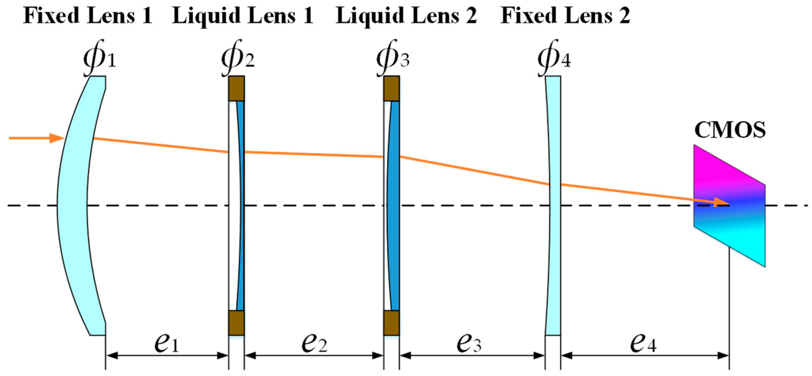
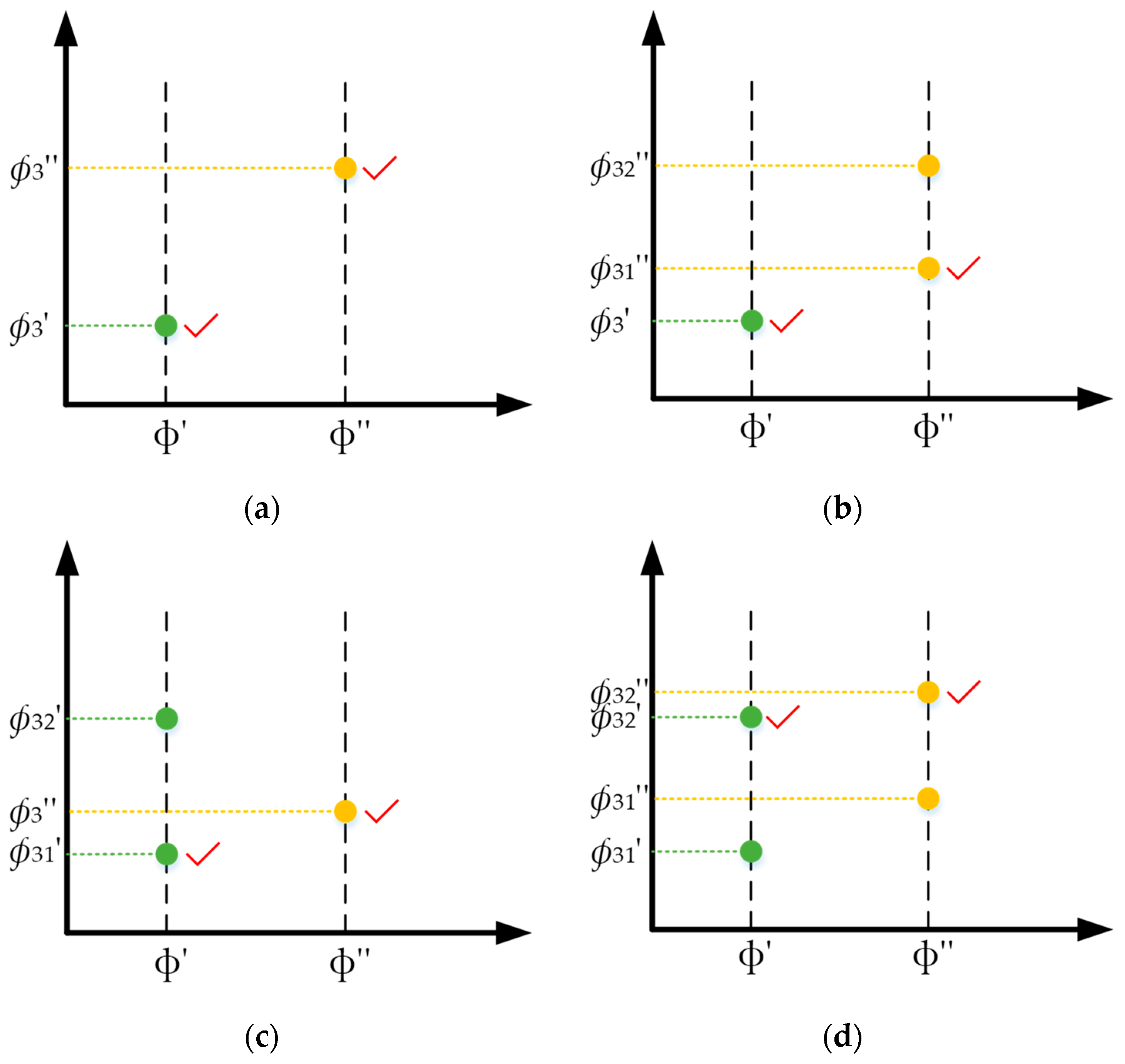
2. Derivation of the Zoom Equation

When designing an optical system, the selection of the initial structure is crucial for achieving the final design requirements. The proposed design refers to the common structure of mechanically compensated zoom systems [20], and the zoom system designed in this paper is composed of four groups. The layout of the zoom system is shown in Figure 1.

In the analysis of thin lens optical systems, the image plane displacement equation as well as the focal power equation of the zoom system can be obtained according to the Gauss bracket method [21] as follows:

$${\mathrm{L}=[ф}_1,-e_1{,ф}_2,-e_2{,ф}_3,-e_3{,ф}_4,-e_4]=0$$

(1)

$${ф=[ф}_1,-e_1{,ф}_2,-e_2{,ф}_3,-e_3{,ф}_4]$$

(2)

In Figure 1 and the aforementioned two equations, L is the image plane displacement and ф is the focal power of the zoom system, ф₁ and ф₄ are the focal power of the fixed lenses, and ф₂ and ф₃ are the focal power of the liquid lenses. Here, e₁, e₂, and e₃ are the distances between each adjacent lens, and e₄ is the distance between the fixed lens 2 and the image plane (CMOS); the object distance was set to infinity.

According to the principle of the Gauss bracket method, we can de-bracket Equation (1) to obtain Equation (3).

$$\begin{gathered} (1-{ф}_1{e}_1)\left[e_2\right(e_3+e_4-e_3{e}_4{ф}_4){ф}_3+(e_2+e_3)e_4{ф}_4-(e_2+e_3+e_4\left)\right]{ф}_2+[1-{ф}_1(e_1+e_2\left)\right](e_3{e}_4{ф}_4-e_3 \\ -e_4){ф}_3+1+{ф}_1{ф}_4{e}_4(e_1+e_2+e_3)-{ф}_4{e}_4-{ф}_1(e_1+e_2+e_3+e_4)=0 \end{gathered}$$

(3)

During the zooming process of the optical system, only ф₂ and ф₃ are variables in Equation (3); so, the functional relation between ф₂ and ф₃ can be further obtained as follows:

$$\begin{array}{c}{ф}_2=g{(ф}_3)=\frac{k_1{ф}_3+k_2}{k_3{ф}_3+k_4}\\ \{\begin{array}{c}{k}_1=\left[{ф}_1\right(e_1+e_2)-1](e_3{e}_4{ф}_4-e_3-e_4)\\ k_2={ф}_1(e_1+e_2+e_3+e_4)+{ф}_4{e}_4[1-{ф}_1(e_1+e_2+e_3\left)\right]-1\\ k_3=(1-{ф}_1{e}_1)(e_3+e_4-e_3{e}_4{ф}_4)e_2\\ k_4=(1-{ф}_1{e}_1)\left[\right(e_2+e_3)e_4{ф}_4-e_2-e_3-e_4]\end{array}\end{array}$$

(4)

Similarly, after removing the brackets of Equation (2), we can obtain the following equation:

$$\begin{gathered} ф=(1-{ф}_1{e}_1\left)\right[e_2(e_3{ф}_4-{1)ф}_3-{ф}_4(e_2+e_3{)+1]ф}_2+\left(e_3{ф}_4-1\right)[{ф}_1\left(e_1+e_2)-1\right]{ф}_3 \\ -{ф}_1{ф}_4(e_1+e_2+e_3{)+ф}_1+{ф}_4 \end{gathered}$$

(5)

Then Equation (4) is substituted into Equation (5) to obtain the functional relation between ф and ф₃ as follows:

$$\begin{array}{c}0=(k_1{k}_5+k_3{k}_7{)ф}_3{}^2+(k_1{k}_6+k_2{k}_5+k_3{k}_8+k_4{k}_7-k_3{ф)ф}_3+k_2{k}_6+k_4{k}_8-k_4ф\\ \{\begin{array}{c}{k}_5=(1-{ф}_1{e}_1)(e_3{ф}_4-1)e_2\\ k_6=(1-{ф}_1{e}_1)[1-{ф}_4(e_2+e_3\left)\right]\\ k_7=(e_3{ф}_4-1)\left[{ф}_1\right(e_1+e_2)-1]\\ k_8={ф}_1+{ф}_4-{ф}_1{ф}_4(e_1+e_2+e_3)\end{array}\end{array}$$

(6)

Equation (6) is essentially a quadratic equation with one unknown about ф₃. Therefore, solving for ф₃ when ф is known requires a discussion of subcases. However, before we start the sub-case discussion, we need to further simplify Equation (6), as shown in Equation (7).

$$\begin{array}{c}0=a{ф}_3{}^2+(b-k_3{ф)ф}_3+c-k_4ф\\ \{\begin{array}{c}a=k_1{k}_5+k_3{k}_7 \\ b=k_1{k}_6+k_2{k}_5+k_3{k}_8+k_4{k}_7\\ c=k_2{k}_6+k_4{k}_8 \end{array}\end{array}$$

(7)

• $a=0$;

In this case, Equation (7) is a linear equation with one unknown about ф₃, and the relation shown in Equation (8) can be obtained by shifting items and other operations.

$${ф}_3=\frac{k_4ф-c}{b-k_3ф}$$

(8)

2.

$\Delta ={\left(b-k_3ф\right)}^2-4a\left(c-k_4ф\right)=0$;

In this case, Equation (7) is a quadratic equation with one unknown about ф₃. However, two equal real roots exist, which can be expressed as follows:

$${ф}_3=\frac{k_3ф-b\pm \sqrt{\Delta }}{2a}=\frac{k_3ф-b}{2a}$$

(9)

3.

$\Delta ={\left(b-k_3ф\right)}^2-4a\left(c-k_4ф\right)>0$;

In this case, although Equation (7) is a quadratic equation about ф₃, two real roots of different magnitudes exist, which can be expressed as follows:

$$\{\begin{array}{c}{ф}_{31}=\frac{k_3ф-b-\sqrt{\Delta }}{2a}\\ {ф}_{32}=\frac{k_3ф-b+\sqrt{\Delta }}{2a}\end{array}$$

(10)

Because the focal power of a liquid lens can only vary within a certain range, the root that does not satisfy the requirement should be discarded. ф₂ corresponding to ф₃ should also be solved according to Equation (4), and if only ф₂ and ф₃ are consistent with the requirement, then the value of ф₃ is reasonable. However, if both ф₃₁ and ф₃₂ are efficient roots, selecting one root between these two roots is crucial because a ф value should correspond to only one ф₃ value when the zoom system is working. Figure 2 shows all possible root distributions of ф₃ for adjacent ф values.

In Figure 2, we used ф′ and ф″ to denote two adjacent ф values and ф₃’ and ф₃″ to denote the corresponding ф₃ values. Figure 2a shows the simplest case with only one ф₃ value corresponding to ф, and no choice problem exists. Figure 2b shows that only one ф₃′ value corresponding to ф′ exists; however, two ф₃″ values, namely, ф₃₁″ and ф₃₂″, corresponding to ф″ exist. Considering the application of liquid lenses in a zoom system, the focal power change in the liquid lens should be made as smooth as possible [13]. Therefore, given that ф₃₁″ is closer to ф₃’ than ф₃₂″, the appropriate value of ф₃″ should be ф₃₁″. Based on this reasoning, the appropriate ф₃’ and ф₃″ values are marked with red check marks in the cases indicated in Figure 2c,d.

4.

$\Delta ={\left(b-k_3ф\right)}^2-4a\left(c-k_4ф\right)<0$;

In this case, no real root of Equation (7) exists with respect to ф₃.

In summary, we have discussed Equation (6) in detail by sub-case so that a ф value always corresponds to only one ф₃ value, and this creates the condition for the solution of the initial structure of the zoom system subsequently.

3. Solution of the Initial Structure

Figure 3 illustrates the process of determining the initial structure of the zoom system. First, the solution space of the zoom system’s structural parameters can be obtained by setting appropriate boundary conditions. Each orange point in the solution space represents a set of structural parameters of the zoom system (i.e., the determined e₁, e₂, e₃, e₄, ф₁, and ф₄). Next, each parameter point in the solution space is evaluated by establishing a suitable evaluation function, and the parameter point with the highest evaluation value (shown as the purple point in Figure 3) corresponds to the optimal initial structure. In the following, the design index of the zoom system is first introduced; next, the process of solving the optimal initial structure is described in detail.

3.1. Design Index

The image sensor selected for this design has a pixel size of 10 μm × 10 μm, corresponding to a Nyquist frequency of 50 lp/mm. The zoom system is a telescopic objective, which is designed for focal length variations of 88–204 mm and field of view (FOV) variations of 1.6–3°. Other design indexes of the zoom system are presented in

Table 1. Design index of the zoom system.

Parameters	Values
Focal length	88–204 mm
F number	8.8–20.4
Field of view	1.6–3°
Working spectrum	486–656 nm
Distortion	≤2
MTF (50 lp/mm)	≥0.2

.

3.2. Solution Space and Evaluation Function

The initial structure of the zoom system exists in the six-dimensional space, as presented in Equation (11). Boundary condition 1 is that when the focal power of the zoom system changes, the focal power of both liquid lenses should not exceed their respective allowable range of variation. Because the focal power of the liquid lens selected for this design varies between −10 and 10 diopter, boundary condition 1 is as presented in Equation (12). To a general non-wide-angle zoom optical system, the focal power of the first group is usually positive [2]. Therefore, boundary condition 2 requires that the focal power of the first group is positive, as shown in Equation (13).

$$\mathrm{A}=\{\left(e_1,e_2,e_3,e_4,{ф}_1,{ф}_4\right)| e_1>0,e_2>0,e_3>0,e_4>0\}$$

(11)

$$\forall ф\in [\frac{1000}{204},\frac{1000}{88}],{ф}_2\in \left[-10,10\right]{\mathrm{and}ф}_3\in \left[-10,10\right]$$

(12)

$${ф}_1>0$$

(13)

It should be noted that any set of structural parameters in the solution space that satisfies the boundary conditions is an initial structural feasible solution for the zoom system. However, good and bad parameters exist among the feasible initial structures. Therefore, establishing an evaluation function is critical for evaluating various initial structures and subsequently finding the initial structure with the highest evaluation value by some search algorithm. In the following, we will give the initial structure evaluation function proposed in this paper, as shown in Equation (14).

$$\mathsf{ƞ}=Value\left(S_{\mathrm{I}},S_{\mathrm{II}},S_{\mathrm{III}},S_{\mathrm{IV}}\right)=\frac{{\omega }_1}{S_{\mathrm{I}}}+\frac{{\omega }_2}{S_{\mathrm{II}}}+\frac{{\omega }_3}{S_{\mathrm{III}}}+\frac{{\omega }_4}{S_{\mathrm{IV}}}$$

(14)

$$\{\begin{array}{c}{S}_{\mathrm{I}}={ф}_1 \\ S_{\mathrm{II}}={\displaystyle \sum _{i=1}^4}{e}_i \\ S_{\mathrm{III}}=\frac{{\sum }_{t=0}^N\left(\right|{ф}_2^t-{ф}_2^{t-1}|+|{ф}_3^t-{ф}_3^{t-1}\left|\right)}{N}\\ S_{\mathrm{IV}}=|{ф}_1|+|{ф}_4|+\frac{{\sum }_{t=0}^N\left(\right|{ф}_2^t|+|{ф}_3^t\left|\right)}{N+1}\end{array}$$

The proposed evaluation function consists of four terms, ф₂^t and ф₃^t in S_III and S_IV are the focal power of liquid lenses 1 and 2 corresponding to ф^t in state t, respectively. Here, ф^t is the focal power of the zoom system in state t, and the zoom system has a total of N + 1 states in the order of uniformly increasing focal power. The smaller S_I is, the smaller the position chromatic aberration and magnification chromatic aberration of the zoom system are [3]. Smaller S_II causes a shorter total length of the zoom system. The smaller the S_III, the smoother the change in the focal power of the liquid lenses. Here, S_IV indicates the field curvature aberration of the zoom system. Because this aberration cannot be well corrected only by optical design software, it must be controlled during the initial structure solving phase [15]. In addition, ω₁, ω₂, ω₃, and ω₄ are the weighting coefficients of S_I, S_II, S_III, and S_IV, respectively.

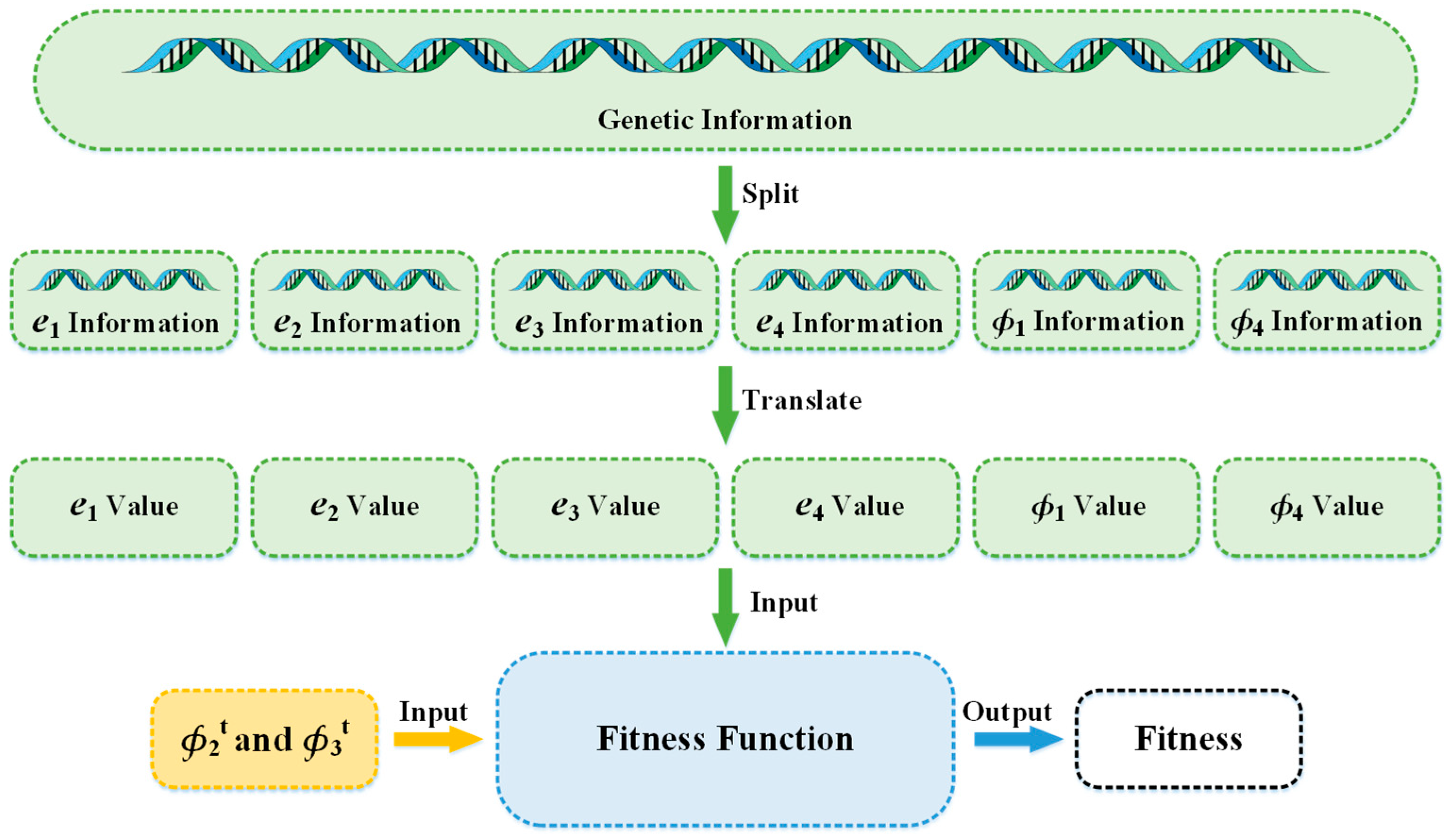
3.3. Genetic Algorithm

The genetic algorithm (GA) is a method to search for the global optimal solution by simulating the natural evolutionary process [22,23]. The method consists of the following three procedures, namely, initialization, fitness calculation, and evolution, as shown in Figure 4a. Furthermore, because some terms are used in this subsection, these terms should be defined.

• Gene: Each variable of the optimization problem is represented by a fixed length string of 0’s and 1’s, which is called a gene;
• Chromosome: All these genes, which represent all the variables, collectively form a chromosome;
• Individual: Chromosomes may also be referred to as individuals in GA;
• Population: Collection of individuals;
• Genetic information: Binary encoding information of the chromosome;
• Genotype: Binary code of the chromosome;
• Phenotype: Values of variables corresponding to the genotype.

3.3.1. Initialization

The initialization procedure of GA includes the selection of the initial population and the determination of parameters such as the evolving algebra. The values of parameters in GA are presented in

Table 2. Values of parameters in GA.

Parameters	Values
Population Size	1000
Chromosome Size	109
Cross Rate	0.8
Mutation Rate	0.003
Evolving Algebra	500

.

The genetic information on each individual chromosome in the initial population consists of a randomly generated binary code. Furthermore, because six structural parameters (e₁, e₂, e₃, e₄, ф₁, and ф₄) are to be solved in this subsection, the genetic information of each chromosome should be segmented so that the segmented six genes correspond to these six parameters, respectively. After that, the genotypes are translated according to an appropriate rule to obtain the values of the corresponding parameters. Finally, the fitness of each chromosome is obtained by substituting these six parameters as well as ф₂^t and ф₃^t into the fitness function. The aforementioned process is shown in Figure 5, and the translation rule mentioned will be explained below.

The long string of binary code at the top in Figure 6 is the genotype (109 binary digits) of a chromosome, which can be divided into six genes. The first five genes (gene e₁, gene e₂, gene e₃, gene e₄, and gene ф₁) were divided by vertical dashed lines into the first 8 and last 10 binary bits. Among them, the first 8 bits corresponded to the integer bits of the corresponding parameter through the conversion rule between binary and decimal, and the last 10 bits corresponded to the decimal bits of the corresponding parameter through the same conversion rule. Because the value of ф₄ could be positive or negative, the gene ф₄ required an additional sign bit, which was the first binary bit divided by a vertical dashed line. If the binary digit of the first bit in gene ф₄ is one, then the value of ф₄ is positive, and vice versa, which means that the value of ф₄ is negative.

3.3.2. Fitness Function

In GA, the probability of a chromosome being inherited by the next generation is determined by the magnitude of the fitness of the chromosome. The greater the fitness of a chromosome is, the greater the probability that the chromosome will be inherited by the next generation; conversely, the smaller the fitness of a chromosome is, the smaller the probability that the chromosome will be inherited by the next generation. Therefore, the fitness value in GA should be non-negative. Considering that the higher the value of the evaluation function in Equation (14), the better the initial structure of the zoom system, we decided to set Equation (14) as the fitness function.

3.3.3. Evolution

Population evolution consists of three genetic operators, namely, selection, crossover, and mutation. The selection step entails eliminating chromosomes with lower fitness values from each generation of the population and retaining only those with higher fitness values. During selection, chromosomes in the population are randomly and reproducibly selected α times, and the genetic information in those selected chromosomes can be inherited by the next generation (the same chromosome may be selected multiple times). It should be noted that the probability of each chromosome in the population being selected was determined by the ratio of the chromosome’s fitness to the population’s total fitness, i.e., Equation (15).

$$P_i=\frac{F_i}{{\sum }_{i=1}^{\alpha }{F}_i}$$

(15)

where P_i is the probability of the chromosome being selected, F_i is the fitness of the chromosome, and α is the population size. It is evident that the higher the fitness value of a chromosome, the higher the probability that it will be selected.

After the selection step, α chromosomes of the parent generation could be obtained. These chromosomes were traversed to obtain parent 1, and parent 2 was obtained by randomly selecting a chromosome among these chromosomes. Crossover and mutation between parents 1 and 2 were performed according to the following rule, resulting in the child chromosome.

• Crossover: When parent 1 crosses with parent 2, a random mask code of equal length with the chromosome’s genotype is generated. When a bit in the mask code is one, the corresponding bit of the child chromosome will inherit the information of that bit in parent 1; when a bit in the mask code is zero, the corresponding bit of the child chromosome will inherit the information of that bit in parent 2.
• Mutation: Each binary digit in the genotype of the child chromosome is mutated with a certain probability (mutation rate): one becomes zero or zero becomes one.

After the aforementioned steps, the children generation with α chromosomes could be obtained. This process of genetic evolution was cyclical until it ended when the termination conditions were satisfied. Figure 7 shows a schematic of the aforementioned crossover and mutation steps, in which the genotype of parent 1 is represented by black numbers, the genotype of parent 2 is represented by white numbers, and the corresponding bits where the mutation occurs are represented by red numbers.

3.3.4. Solution

Equation (14) presents the initial structure evaluation function proposed in this paper, where the values of ω₁, ω₂, ω₃, and ω₄ reflect the importance of S_I, S_II, S_III, and S_IV, respectively. These four weighting coefficients as well as N should be determined by experimental adjustment. For example, if S_II is always too large during the search of GA, the value of ω₂ should be increased appropriately. Finally, the initial structural parameters of the zoom system can be obtained after the search of GA. The solving result is presented in

Table 3. Solving result for structural parameters.

Parameters	Values
$e_1$	37.3 mm
$e_2$	95.598 mm
$e_3$	64.619 mm
$e_4$	35.316 mm
${ф}_1$	6.071 diopter
${ф}_4$	8.174 diopter

. In the evaluation function, ω₁ was set to 1, ω₂ was set to 10, ω₃ was set to 18, ω₄ was set to 5, and N was set to 646.

4. Optimized Design Results and Discussion

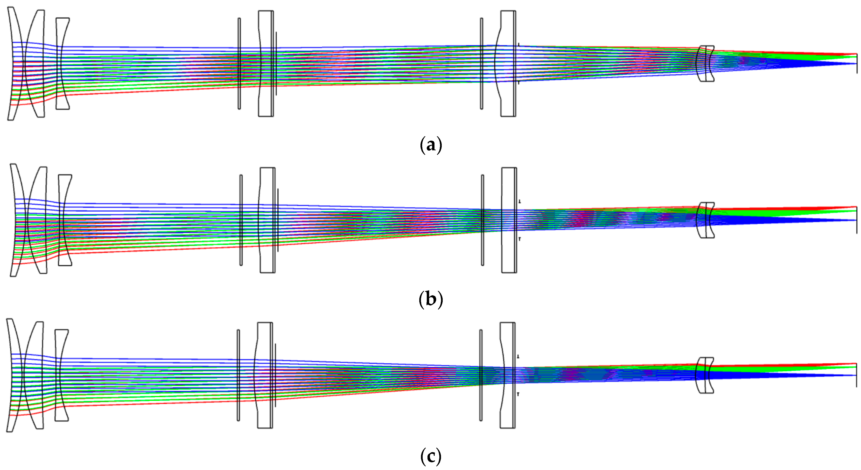
4.1. Optimized Design of the Zoom System

The initial structural parameters obtained in the aforementioned section were substituted into the optical design software Zemax [24] to optimize the optical system. Thus, the ideal optical system was converted into an actual optical system. The final structure of the zoom system is shown in Figure 8, and the lens data are listed in

Table 4. Lens data results for the zoom system.

Surface	#	Radius (mm)	Thickness (mm)	Material
object		Infinity	Infinity
Fixed Group 1	1	−73.263	2.404	E-LLF6
	2	−39.564	0.500
	3	28.744	4.274	H-ZLAF55F
	4	260.310	3.296
	5	−228.547	0.900	CAWO4-E
	6	26.941	41.998
Liquid Lens 1	7	Infinity	0.500	D263T
	8	Infinity	zoom
	9	zoom	zoom	OL1224_VIS
	10	Infinity	0.500	D263T
	11	Infinity	0.700
	12	Infinity	48.423
Liquid Lens 2	13	Infinity	0.500	D263T
	14	Infinity	zoom
	15	zoom	zoom	OL1224_VIS
	16	Infinity	0.500	D263T
	17	Infinity	0.700
	18	Infinity	41.998
Fixed Group 2	19	8.850	2.249	D-LAF50
	20	58.608	0.900	LF5G15
	21	6.105	34.998
Image		Infinity

. It should be noted that during the zooming process of the optical system, only the focal power of the two liquid lenses changed. The total length of the system was 200 mm, and the focal length was 88.3547–204.62 mm. Furthermore, both liquid lenses used in our design were from Optotune [25] (Product series: EL-16-40-TC-VIS-20D-1-C (Edmund Optics, Barrington, IL, USA)).

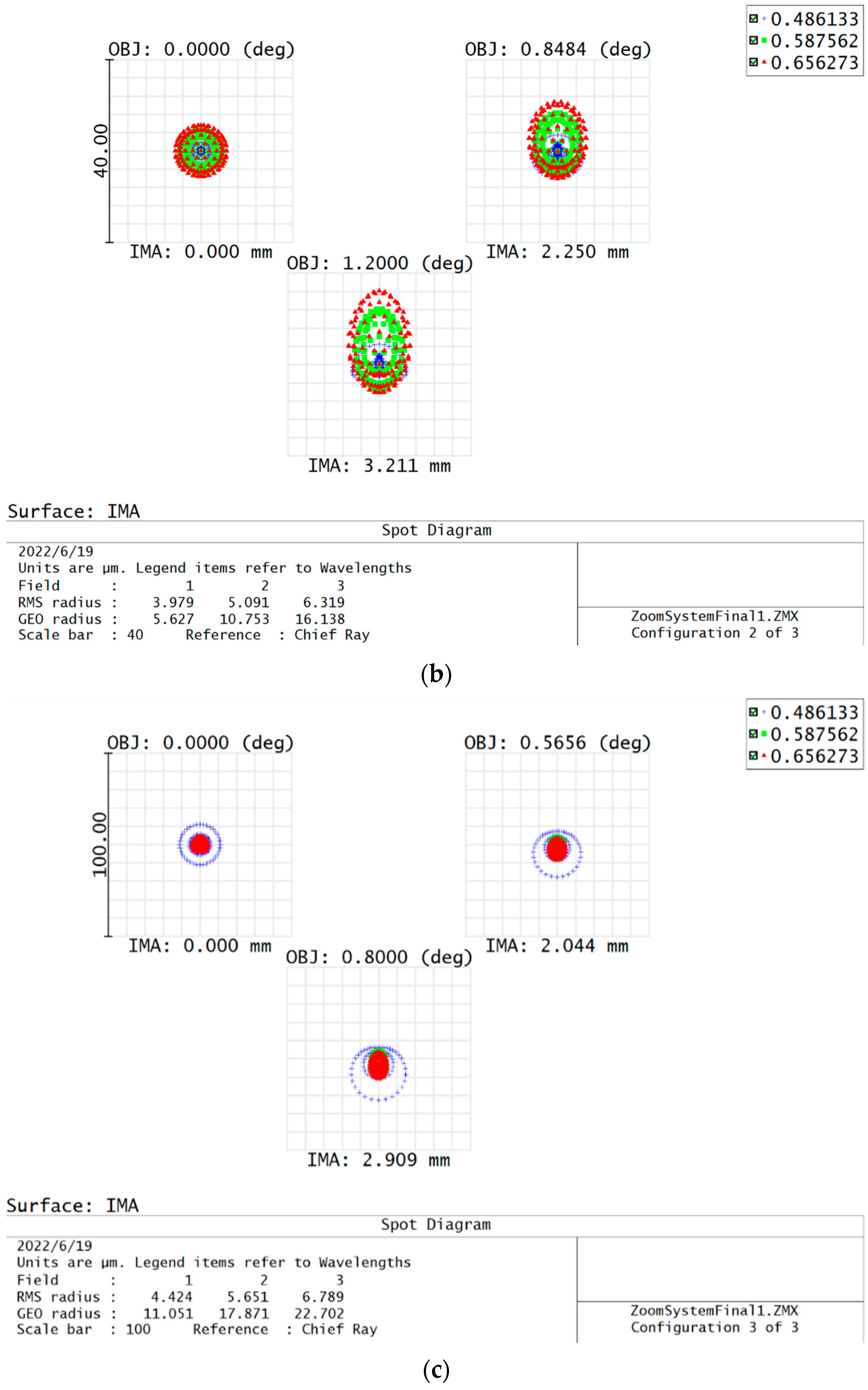
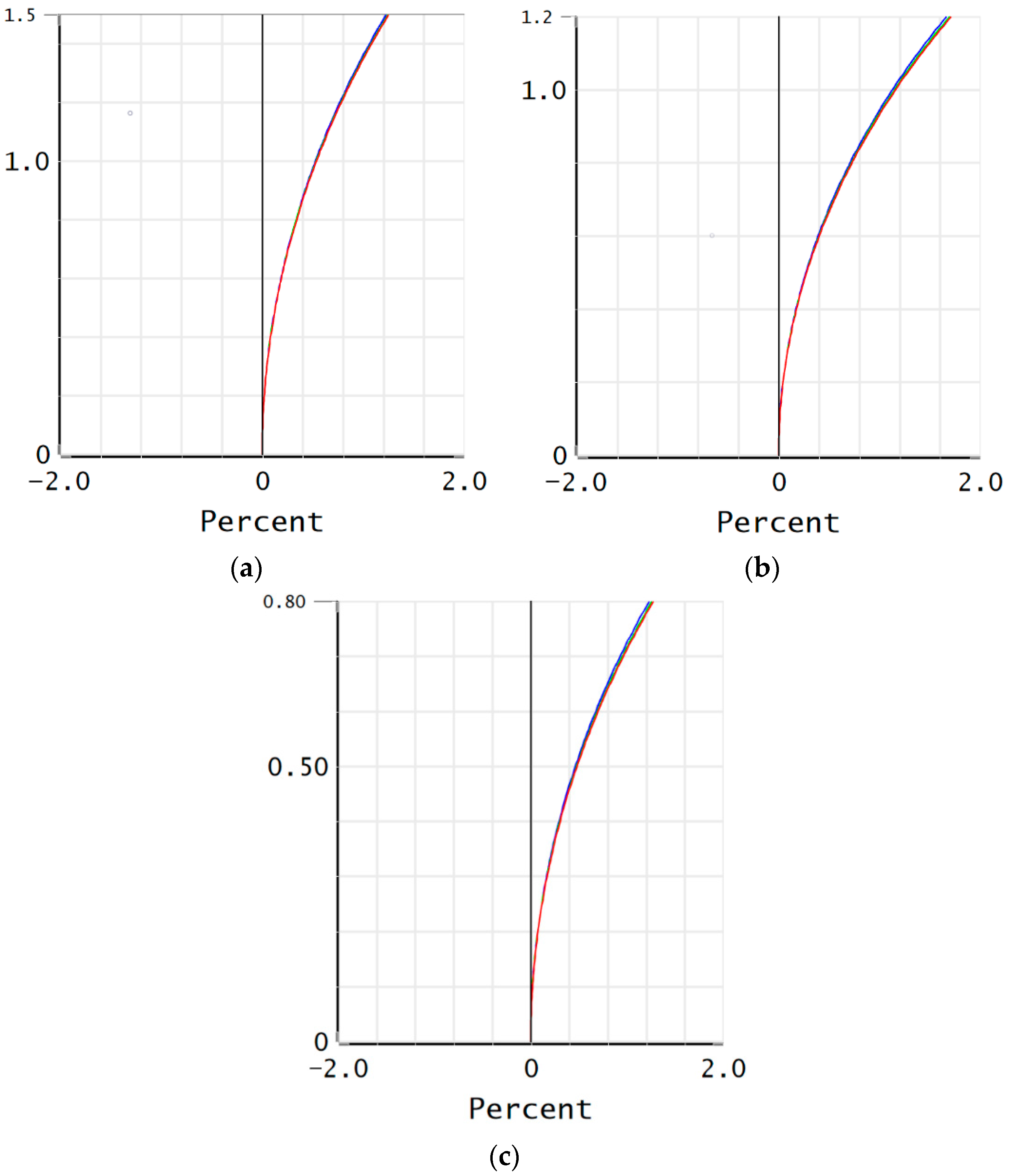
4.2. Image Quality Evaluation

The modulation transfer function (MTF), spot diagram, and distortion are critical indicators for evaluating the image quality of an optical system [3]. MTF is a comprehensive evaluation indicator and can objectively reflect the imaging process, characteristics, and image quality of the optical system. Subplots (a)(b)(c) in Figure 9 detail the MTF curves of the zoom system at short focal length, medium focal length, and long focal length, respectively. Obviously, the MTFs at three focal lengths are greater than 0.2 at the Nyquist frequency (50 lp/mm), and all are close to their respective diffraction limits. The spot diagram can accurately reflect the diffusion of imaging light for an optical system. Subplots (a)(b)(c) in Figure 10 correspond to the spot diagrams of the zoom system at three focal lengths, respectively. It can be seen that the root mean square (RMS) radii of all three spot diagrams are small, which represents a better imaging quality of the optical system. Although the distortion does not affect the sharpness of the image, it can cause image deformation. Figure 11 shows the distortion of the zoom system, and as can be seen, the distortions of the zoom system are less than 2% at all three focal lengths. The aforementioned analysis results reveal that the designed zoom optical system exhibits an excellent imaging capability.

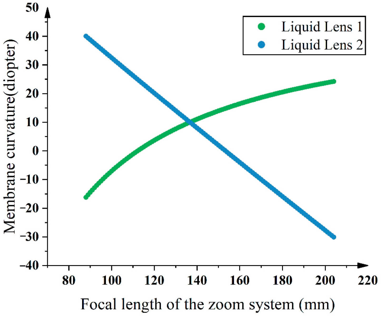
4.3. Zoom Curve Analysis

Using optical design software Zemax, the change in membrane (an element that can change the focal power of liquid lenses) curvatures of liquid lenses 1 and 2 was observed during the zooming process of the optical system, as shown in Figure 12. It can be seen that the membrane curvature of liquid lens 2 decreases linearly, so liquid lens 2 essentially acts to change the focal length of the optical system. The liquid lens 1 exhibits a nonlinear increase in membrane curvature, which acts to compensate for the image plane displacement. The membrane curvatures of both liquid lenses change smoothly, indicating that the zoom system can achieve smooth and continuous zooming.

4.4. Tolerance Analysis

After designing the optical system, performing tolerance analysis is crucial. By considering the tolerance sensitivity of each optical element of the zoom system at short focal length, medium focal length, and long focal length, the tolerance distribution of the zoom system is presented, as shown in

Table 5. Tolerance distribution of the zoom system.

Tolerance Items	Values
Radius/fringe	≤3
Thickness/mm	±0.02
Surface decenter/mm	±0.02
Element tilt/°	±0.02
Element decenter/mm	±0.02
Surface irregularity/fringe	≤0.3
Refractive index	±0.001
Abbe number/%	±0.5

. Furthermore, using the tolerance analysis function in Zemax, a Monte Carlo analysis probability diagram of the zoom system was obtained at 50 lp/mm, as shown in Figure 13. Here, 90% of the zoom systems exhibit MTFs greater than 0.2 in the zoom range, which indicates that the tolerance distribution presented in Table 5 is appropriate for the actual production and manufacture of the designed zoom system.

5. Conclusions

In this paper, an automatic search method of global optimal initial structure based on GA was proposed for improving the initial structure design of complex optical systems. This method can provide researchers with a great starting point for optical system design and is a useful exploration of using artificial intelligence techniques to automate the design of complex optical systems. By applying this method, we designed a telescopic optical system with flexible zoom capability. The designed optical system allows fast and smooth zooming and has a simple structure that can be manufactured easily. The zoom range of the optical system is 88.3547–204.62 mm, and the FOV is 1.6–3°. The imaging performance indexes (including MTF, spot diagram, and distortion) indicate that the optical system exhibits excellent imaging capability and image quality.

References

1. Li, H.; Cheng, X.; Hao, Q. An Electrically Tunable Zoom System Using Liquid Lenses. Sensors 2015, 16, 45. [Google Scholar] [CrossRef] [PubMed] [Green Version]
2. Zhang, K.; Qu, Z.; Zhong, X.; Li, F.; Yu, S. 40× zoom optical system design based on stable imaging principle of four groups. Appl. Opt. 2022, 61, 1516–1522. [Google Scholar] [CrossRef] [PubMed]
3. Zhang, K.; Zhong, X.; Qu, Z.; Meng, Y.; Su, Z. Design method research of a radiation-resistant zoom lens. Opt. Commun. 2022, 509, 127881. [Google Scholar] [CrossRef]
4. Qu, R.; Duan, J.; Liu, K.; Cao, J.; Yang, J. Optical Design of a 4× Zoom Lens with a Stable External Entrance Pupil and Internal Stop. Photonics 2022, 9, 191. [Google Scholar] [CrossRef]
5. Cheng, X.; Ye, H.; Hao, Q. Synthetic system design method for off-axis stabilized zoom systems with a high zoom ratio. Opt. Express 2021, 29, 10592–10612. [Google Scholar] [CrossRef] [PubMed]
6. Wang, J.; Amani, A.; Zhu, C.; Bai, J. Design of a compact varifocal panoramic system based on the mechanical zoom method. Appl. Opt. 2021, 60, 6448–6455. [Google Scholar] [CrossRef]
7. Cao, C.; Liao, Z.; Bai, Y.; Xing, T. Design of large zoom ratio long-wave infrared zoom system with compound zoom method. Opt. Eng. 2018, 57, 025104. [Google Scholar]
8. Li, L.; Wang, D.; Liu, C.; Wang, Q. Zoom microscope objective using electrowetting lenses. Opt. Express 2016, 24, 2931–2940. [Google Scholar] [CrossRef] [PubMed]
9. Miks, A.; Novak, J. Analysis of two-element zoom systems based on variable power lenses. Opt. Express 2010, 18, 6797–6810. [Google Scholar] [CrossRef]
10. Miks, A.; Novak, P. Paraxial design of four-component zoom lens with fixed position of optical center composed of members with variable focal length. Opt. Express 2018, 26, 25611–25616. [Google Scholar] [CrossRef] [PubMed]
11. Jiang, Z.; Wang, D.; Zheng, Y.; Liu, C.; Wang, Q. Continuous optical zoom microscopy imaging system based on liquid lenses. Opt. Express 2021, 29, 20322–20335. [Google Scholar] [CrossRef] [PubMed]
12. Li, L.; Yuan, R.; Wang, J.; Wang, Q. Electrically optofluidic zoom system with a large zoom range and high-resolution image. Opt. Express 2017, 25, 22280–22291. [Google Scholar] [CrossRef] [PubMed]
13. Liu, Y.; Yang, B.; Gu, P.; Wang, X.; Zong, H. 50X five-group inner-focus zoom lens design with focus tunable lens using Gaussian brackets and lens modules. Opt. Express 2020, 28, 29098–29111. [Google Scholar] [CrossRef] [PubMed]
14. Hao, Q.; Cheng, X.; Du, K. Four-group stabilized zoom lens design of two focal-length-variable elements. Opt. Express 2013, 21, 7758–7767. [Google Scholar] [CrossRef] [PubMed]
15. Yu, X.; Wang, H.; Yao, Y.; Tan, S.; Xu, Y.; Ding, Y. Automatic design of a mid-wavelength infrared dual-conjugate zoom system based on particle swarm optimization. Opt. Express 2021, 29, 14868–14882. [Google Scholar] [CrossRef] [PubMed]
16. Fan, Z.; Wei, S.; Zhu, Z.; Mo, Y.; Yan, Y.; Ma, D. Automatically retrieving an initial design of a double-sided telecentric zoom lens based on a particle swarm optimization. Appl. Opt. 2019, 58, 7379–7386. [Google Scholar] [CrossRef] [PubMed]
17. Fan, Z.; Wei, S.; Zhu, Z.; Yan, Y.; Mo, Y.; Yan, L.; Ma, D. Globally optimal first-order design of zoom systems with fixed foci as well as high zoom ratio. Opt. Express 2019, 27, 38180–38190. [Google Scholar] [CrossRef]
18. Pal, S.; Hazra, L. Structural design of mechanically compensated zoom lenses by evolutionary programming. Opt. Eng. 2012, 51, 063001. [Google Scholar] [CrossRef]
19. Carsten, R.; Tarik, G.; Alois, H. Development of an open source algorithm for optical system design, combining genetic and local optimization. Opt. Eng. 2020, 59, 055111. [Google Scholar]
20. Zhou, H.; Liu, Y.; Sun, Q.; Li, C.; Zhang, X.; Huang, J. Mechanically compensated type for midwave infrared zoom system with a large zoom ratio. Opt. Eng. 2013, 52, 013002. [Google Scholar]
21. Herzberger, M. Gaussian Optics and. Gaussian Brackets. J. Opt. Soc. Amer. 1943, 33, 651–655. [Google Scholar] [CrossRef]
22. Katoch, S.; Chauhan, S.S.; Kumar, V. A review on genetic algorithm: Past, present, and future. Multimed. Tools Appl. 2021, 80, 8091–8126. [Google Scholar] [CrossRef] [PubMed]
23. Michalewicz, Z.; Schoenauer, M. Evolutionary Algorithms for Constrained Parameter Optimization Problems. Evol. Comput. 1996, 4, 1–32. [Google Scholar] [CrossRef]
24. Zemax. Available online: https://www.zemax.net.cn/pages/opticstudio/ (accessed on 2 June 2022).
25. Optotune. Available online: https://www.optotune.com/ (accessed on 4 June 2022).
Figure 1. Optical layout of the zoom system.
Photonics 09 00536 g001
Figure 2. Distribution of all possible values of ф3: (a) There is one ф3 value corresponding to each of the adjacent ф values; (b) The former ф value corresponds to one ф3 value, and the latter ф value corresponds to two ф3 values; (c) The former ф value corresponds to two ф3 values, and the latter ф value corresponds to one ф3 value; (d) There are two ф3 values corresponding to each of the adjacent ф values.
Photonics 09 00536 g002
Figure 3. Initial structure solving process of the zoom system.
Photonics 09 00536 g003
Figure 4. (a) Flowchart of GA; (b) Population, individuals, and chromosomes; (c) Parent generation produces children generation through crossover and mutation.
Photonics 09 00536 g004
Figure 5. Fitness-solving process.
Photonics 09 00536 g005
Figure 6. Translation rule.
Photonics 09 00536 g006
Figure 7. Schematic of crossover and mutation.
Photonics 09 00536 g007
Figure 8. Final structure of the zoom system: (a) Focal length of the zoom system is 88.3547 mm; (b) Focal length of the zoom system is 150.096 mm; (c) Focal length of the zoom system is 204.62 mm.
Photonics 09 00536 g008
Figure 9. MTF curves of the zoom system: (a) Focal length of the zoom system is 88.3547 mm; (b) Focal length of the zoom system is 150.096 mm; (c) Focal length of the zoom system is 204.62 mm.
Photonics 09 00536 g009aPhotonics 09 00536 g009b
Figure 10. Spot diagrams of the zoom system: (a) Focal length of the zoom system is 88.3547 mm; (b) Focal length of the zoom system is 150.096 mm; (c) Focal length of the zoom system is 204.62 mm.
Photonics 09 00536 g010aPhotonics 09 00536 g010b
Figure 11. Distortion curves of the zoom system: (a) Focal length of the zoom system is 88.3547 mm; (b) Focal length of the zoom system is 150.096 mm; (c) Focal length of the zoom system is 204.62 mm.
Photonics 09 00536 g011
Figure 12. Zoom curves.
Photonics 09 00536 g012
Figure 13. Probability diagram of Monte Carlo analysis.
Photonics 09 00536 g013