Article

Sustainable Green Economy for a Supply Chain with Remanufacturing by Both the Supplier and Manufacturer in a Varying Market

1
Department of Mathematics, Indian Institute of Engineering Science and Technology, Shibpur, Howrah 711 103, India
2
Doctoral School of Economic and Regional Sciences, Hungarian University of Agriculture and Life Sciences, 2100 Godollo, Hungary
3
Hungarian National Bank—Research Center, John Von Neumann University, 6000 Kecskemet, Hungary
4
Department of Mathematics, Sonarpur Mahavidyalaya, Rajpur, Kolkata 700 149, India
*
Author to whom correspondence should be addressed.
Logistics 2023, 7(3), 37; https://doi.org/10.3390/logistics7030037
Submission received: 12 March 2023 / Revised: 11 May 2023 / Accepted: 31 May 2023 / Published: 4 July 2023
(This article belongs to the Section Sustainable Supply Chains and Logistics)

Abstract

:
Background: In a typical multiechelon supply chain, the supplier makes semifinished items, from which the manufacturer produces finished products to eventually get sold at retailers. However, the majority of existing supply chain models consider the remanufacturing of defective products by solely one organization, despite the fact that both the supplier and manufacturer can produce defective products. This study considers the remanufacturing of defective products with fresh materials and additional expenses by both the supplier and manufacturer. Contrary to well-established articles that hold major partners to be accountable for reducing carbon emissions under a carbon cap-and-trade policy, the proposed model presumes an initial green technological investment by each chain partner. Methods: This study represents a varying market with fuzzy cost components that are then defuzzified with λ -integral method. This study determines the critical values of three discrete and four other continuous decision variables that globally maximize the profitability of the proposed model. Results: Slower production with a longer cycle boosts profitability in a developing market. To increase profit, a case study on the oil and natural gas business suggested to reduce the production of defective items and cutting emission through green investments. Conclusions: Managers can sustainably boost profit via careful production, modern machinery, and slightly longer cycles.

1. Introduction

Bygone is the era of parochial supply chain (SC) networks with unrealistic suppositions, such as perfect quality products, outdated environmental laws, uninformed customers, and a stable market [1]. Even though decision makers (DM) aim for the higher net profit of any SC as a whole, through inte-organizational collaborations on environmental concerns, advertisement policy, sale price, and several other aspects [2], different chain partners are rarely allowed to exchange the obligation to follow the prevailing regulations with others [3]. In real-life-oriented scenarios, the DMs’ standard goal of any SC counts in the orientation, collaboration, and coordination of business processes and activities of various chain partners to ameliorate an all-inclusive account and efficacy [4].
However, SC managers can rarely shift the organizational liabilities of one chain partner to another partner. For example, the phasewise curtailment of the discharge of greenhouse gas (GHG) under the carbon cap-and-trade directive of the Paris Accord is the organization’s obligation, which cannot be passed on to another chain partner of any SC model [5]. While the manufacturing sectors in the USA and other established economies emit approximately 79 % of GHG, emerging economies emit GHG at a faster rate than hitherto. To effectively tackle this issue, several nations worldwide had come together to sign the Kyoto Protocol to honor the concept of common but differentiated accountability regarding carbon emissions (CEs), thereby putting a yearly compulsory limit on CEs [6].
Later, world leaders redesigned the Kyoto Protocol to encompass the Paris Accord, which compels manufacturers in participating nations to implement the carbon cap-and-trade directive to reduce CEs in a timely manner [7]. The DMs across organizations make yearly investments on green machinery and recent technologies to gradually reduce CE-related costs in the framework of the Paris Accord [8]. However, the majority of recent SC studies either determine the optimal investment to be made solely by one chain partner (typically, the manufacturer), or sometimes consider the green investment of various chain partners as a whole [9].
On the other hand, the increased collaborations among different chain partners lead to higher operational efficiency and better profit margins of SCs as a whole [10]. Among the various types of marketing collaboration policies, one well-established implementation approach entails the sharing of certain portions of retailers’ local advertising costs by upper-level chain partners. Researchers term this as a cooperative advertisement policy with unilateral participation, the budgetary aspects of which are crucial to any conventional SC [11]. Nevertheless, there are very few multiechelon SC articles that determine the ideal advertisement budgets of various chain partners to meet certain demand rates of retail customers under the Paris Accord in an uncertain market.
In any archetypal three-echelon SC, the supplier procures the raw materials to produce the semifinished items that are to be transported to the manufacturer [2]. Then, the manufacturer produces the finished products to be procured by the retailers [12]. Undeniably, in any real-life oriented SC, the machinery of both the supplier and manufacturer produces a certain portion of imperfect-quality (i.e., faulty) products [13]. However, the majority of existing SC studies consider the faulty machinery of solely one chain partner (e.g., the manufacturer) while dodging all other processors (e.g., the supplier). Moreover, there are very few existing SC models that consider the remanufacturing of faulty products with extra raw materials by incurring additional costs related to labor and electricity. Another major concern of any business is regarding the uncertainty of the market and the resulting uncertain nature of various cost coefficients [14]. While researchers effectively express those coefficients with a fuzzy set, a natural multivariate-type extension of the classical crisp set [15], they efficiently capture the uncertainty of the market with the degree-of-optimism-based λ -integral method of defuzzification to the asymmetric triangular fuzzy number (TFN)-type parameters [14].
This way, this study identifies a number of gaps in the current SC literature as follows:
  • The majority of existing SC models take the remanufacturing of faulty products by the imperfect machinery of solely one chain partner into account. However, the consideration of the use of fresh raw materials and associated energy- and labor-related costs during the remanufacturing of faulty products by multiple chain-partners is extremely rare.
  • The Paris Accord, together with the growing environmental awareness among the masses, motivates each and every chain partner to invest yearly on advanced green equipment. Nevertheless, only one chain partner had made the initial green technological investment (GTI) under the carbon cap-and-trade regulation in most existing multiechelon SC models.
  • Many SC models were developed subject to the fixed cost components in an uniform market condition, irrespective of the liquidity position of various chain partners. These suppositions are contradictory to real-life scenarios.
All of these intents lead this paper to zero in on recent and well-established articles in the current research area, as discussed in Section 2. Then, the reader can maneuver through the rest of this paper, starting from Section 3, which describes the symbols and the hypotheses relevant to current research. Then, this study formulates the proposed SSCM model in Section 4. Section 5 establishes the global optimality of the proposed model by developing the theorems, and then arrives at some analytical observations. This study numerically explores the applicability of the proposed model in Section 6 through one example, and thereafter, one case study, on oil and natural gas industries. Moreover, this study performs vulnerability analysis and associated managerial acumen for both of these experiments. Furthermore, this section compares the current study with several well-established articles. Section 7 concludes this study and posts a number of future research scopes.

2. Literature Review

This section focuses on the review of recent and well-established articles in the current area of research. Since time immemorial, SC managers have aimed to institutionalize interconnections among different chain partners to earn higher net profits. Thus, this review focuses on three other major segments in the recent SC literature as follows:

2.1. Review of the Environmentally Sustainable SC Models

The growing concerns of the general population, along with the international regulations regarding environmental damages, compel SC managers to embrace CE control mechanisms rather than abandoning them (Mishra et al. [16]). Among the major reviews of environmentally friendly SSCM models, Bazan et al. [17] analytically and extensively studied a large number of logistics models.
Among recent articles, Taleizadeh et al. [18] formulated four independent production inventory models under full and partial backordering and lost sales. These models aimed at maximizing profit while improving the quality of service. Cao and Yu [19] studied the relationships between various economic and operational decisions of an SC model under controllable CEs and cooperation between a manufacturer and a retailer of medium wealth. They suggested that retailers could avoid any loss by ordering products in lesser quantities under the CEs and capital constraints. Wu et al. [20] established a game-theory-based cost-sharing arrangement between manufacturers and retailers to reduce the emissions of GHG under minimum marketing efforts. They figured out that the optimal subsidy policy of the government should be set by measuring its impact on the prevailing cost-sharing plan between manufacturers and retailers. Likewise, to concurrently minimize the total cost and CE-related cost, Babagolzadeh et al. [21] developed a two-stage stochastic cold SC model with carbon tax regulation under demand uncertainty. They conducted a real-life-based case study in Queensland, Australia, and thus determined that the higher CE cost was hindering the profitability of organizations. Garai and Roy [22] discussed a multiobjective optimization method for one customer-centric and cost-effective closed-loop SC in the T-environment.
Very recently, Mishra et al. [16] elaborately discussed four sustainable inventory models with manageable CEs under different backordering criteria. They determined the optimal strategy by jointly considering the yearly investments on recent preservation technology and the GTI scheme. The article by Garai et al. [2] on a closed-loop SC model aimed to determine the cost-saving subsidy policy of growers and biofuel plants while dealing with various herbs and herbal medicines. They developed an interactive optimization algorithm under a real-life-oriented T-environment. However, there was barely any deliberation on the prevailing Paris Accord to reduce CEs in their model. Moreover, the case-study of Homayouni et al. [7] analyzed two controllable CE-related policies, namely the carbon cap-and-trade policy and carbon tax, towards formulating a green supply chain with multisupplier and multicarrier transport. Their heuristic method indicated that the incitement of carbon cap-and-trade policies were highly efficient at cutting CEs. The production and reworking system with a single manufacturer and multiretailer in Malleeswaran and Uthayakumar [23] approved that the consideration of environmental aspects increased the demand rate and consequently surged the profit of all chain partners. Furthermore, the manufacturer had incurred a minimal cost by setting up a green policy and reducing the discrete ordering cost. Here, Table 1 tabulates some other SC studies in this regard.

2.2. Review of SC Models with the Faulty Machinery

A number of recent articles have focused on faulty products from the imperfect machinery of one chain partner within an SC [33]. Recently, Taleizadeh et al. [18] dealt with an inventory model with the imperfect-quality products. Although the rate of imperfectness was a random variable under a specified probability distribution function, the manufacturer needed to outsource faulty products for the reworking of those. Ben-Daya et al. [34] developed an environmentally friendly remanufacturing approach in a two-stage closed-loop SC with one vendor and many buyers. They found that while the vendor’s setup costs increased relative to buyers’ ordering expenses, their model opted to produce more for earning the highest aggregate revenue. Kang et al. [35] employed a single-stage production inventory model with inspection plus a reworking facility to sell only perfect-quality products, thereby upholding the brand image of organization. They prioritized the quality of saleable products over the fulfillment of demand for customers, and thus amalgamated remanufacturing, inspection stations, and planned backordering in their model. The article by Mondal et al. [14] examined an inventory model of seasonal and deteriorating products in a competitive market. While they determined the corresponding global optimal solution in a neutrosophic environment, they advocated for a cost reduction in early promotions to initially portray the lower demand rate.
Recently, Chambari et al. [36] developed a simulation-based bi-objective optimization algorithm. Thus, they determined the optimal solution to the redundancy allocation problem under imperfect switching. Around the same time, Khara et al. [37] advanced the imperfect inventory study by formulating a two-layer SC model subject to time-varying development costs. The model could preserve the products’ reliability by lowering the rate of imperfectness of finished products for the manufacturer, thereby generating a higher net profit along with an optimal production and replenishment cycle. Giri and Dash [30] formulated one imperfect production inventory model with an error-free screening process of the retailer after receiving products from the manufacturer. They determined the optimal pricing, advertising, and inventory decisions by applying the Stackelberg gaming approach on both the centralized and decentralized models. They suggested implementing a cost-sharing contract between the manufacturer and retailer to significantly enhance the profitability, green aspects, and frequency of the advertisement. Table 1 conscripts some other major articles in this regard.

2.3. Review of Various Advertising Policies of SC Models

Worldwide economic globalization and highly unpredictable demands from customers signify the scopes of collaboration and cooperation in various aspects for chain partners of any SC model [4].
Among recent analytical reviews of cooperative advertising-based SC studies, readers can explore the article by Daryanto et al. [12], who developed a three-echelon SC model with a transportation-related CE cost subject to the disposal of deteriorated products. They optimally determined the supplier’s delivery policy by minimizing GHG emissions, and found that fuel consumption affects both aggregate costs and GHG emissions. Around the same time, Sarkar et al. [10] also expanded the concepts of cooperative advertising among a sole supplier, sole manufacturer, and multiple retailers under the variable demand rate. They presumed all basic costs to be fuzzy in nature, and thereby maximized the aggregate revenue of the entire SC. Zhang et al. [38] studied the balancing strategies by considering the subsiding decisions and manufacturer’s influences in a two-echelon SC. Among the various types of channel structures, such as direct, dual, and retail, they observed that both chain partners preferred to invest in the CE reduction directive under a single-channel structure subject to ecofriendly preferences for customers. Li et al. [39] examined the effects of the cooperative marketing policy of the online-to-offline SC with a lift-products strategy. While this system could avoid the incentive effects of cooperative marketing, they find the cooperative advertisement policy to be beneficial only under certain circumstances.
Of late, Khorshidvand et al. [11] has discussed the coordination policy in multichannel and multilevel SCs by considering several major concerns, including cost, environment, and marketing, in both online and traditional channels. They corroborated several instances, and thereby analyzed a suggested nonlinear optimization model. The article by Soleimani et al. [40] focused on various advertisement-related aspects, and thus determined the sustainable strategies of a closed-loop SC with energy efficiency. They developed a set of efficient Lagrangian relaxation reformulations, along with fast heuristics, to solve their model. Around this time, Peng et al. [41] considered green investment to promote the low-carbon products in an SC with various incentives. While they observed that GTI induced a reduction in emissions of GHGs, they recommended legislators, manufacturers, and retailers to be cooperative for the effective promotion of low-carbon products. Moreover, they suggested manufacturers to use recent technologies in the production process. Here, Table 1 enlists some other key contributions in this research area.

2.4. Current Contributions

This review of current and well-established SC articles exhibits the scopes to accommodate the present study with the following major contributions:
  • To formulate a three-echelon SSCM model with a single supplier, a single manufacturer, and multiple retailers with the faculty machinery of the supplier and manufacturer, both subject to the unilateral cooperative advertisement policy and the solitary carbon cap-and-trade regulation of the Paris Accord for each and every chain partner in uncertain market. Moreover, to consider the instantaneous remanufacturing of defective products with supplementary raw materials by incurring additional labor- and energy-related costs to the faulty machinery of both the supplier and manufacturer of the proposed model.
  • Subject to certain demand rates of retail customers across retailers, to determine the ideal cooperative advertising budgets and the optimal amounts of GTI of each and every chain partner in an uncertain market, thus proposing some useful policies for the economic and environmental sustainability of the proposed SSCM model. Correspondingly, to find out the optimal cycle lengths of all chain partners, along with the production rates and numbers of dispatchable units for the supplier and manufacturer of the proposed model.
  • To perform sensitivity analysis of some significant parameters of the proposed SSCM model and afterwards, to extract some managerial acumen.

3. Model Specifications

3.1. Notations with Descriptions

Table 2 enlists several useful notations and their descriptions in connection with the formulation of the proposed model.

3.2. Assumptions

In order to determine some sustainable green economic policies for the proposed SC model with multiple faulty productions, this study makes the following assumptions:
i. The imperfect production systems of the supplier and manufacturer produce some defective items alongside perfect-quality deliverables. However, the intelligent production systems of those chain partners perfectly identify the defective items and direct them toward immediate remanufacturing, thus upholding their brand images. This study takes into account the cost per unit of the aforementioned production process, which happens to be affected by the production rate, and is borne by the supplier and manufacturer as follows [42]:
c 0 ( P p ) = c ¯ 0 p + α p P p + c ¯ d c p P p , P p > 0 , p : supplier or manufacturer .
ii. This study addresses the essential requirement for fresh raw materials to remanufacture those defective items, a subject that has hardly been covered in existing articles. Any typical remanufacturing requires only a certain percentage of the raw materials that were initially needed to produce the item. Thus, considering the additional raw materials ω p as κ μ p μ p and associated labor- and energy-related costs as c ˜ 0 p to remanufacture each defective item, this study derives the unit remanufacturing cost for faulty products at any chain partner ( S R p ) as follows:
S R p = c ¯ d p + ω p c ¯ 0 p , c ¯ 0 p = c 0 p + 1 2 ( δ c 0 2 p λ δ c 0 1 p λ δ c 0 2 p ) , c ¯ d p = c d p + 1 2 ( δ c d 2 p λ δ c d 1 p λ δ c d 2 p ) .
iii. Globally, there is huge concern over the rapid increase in GHG levels, which causes special difficulties for the continuation of life as we know it on Earth. Almost all countries have come together in support of the Paris Accord, an international treaty, in response to this pressing issue. As a result, businesses that produce, ship, or store a variety of products must adhere to the Paris Accord’s carbon cap-and-trade system. Correspondingly, at the start of each year, each and every chain partner of the proposed model has to purchase some carbon credits that allow the owner to emit a specific quantity of GHGs. In contrast to this strategy, which demands frequent financial contributions from chain partners, researchers have found that CEs can be gradually reduced and regulated by installing and/or upgrading green machinery and recent software [43]. Researchers have termed the said self-contained monetary investment by each chain partner as green technological investment (GTI) (see Mishra et al. [16], Mishra et al. [6]).
iv. The unilateral cooperative advertisement policy encourages each chain partner to contribute a specific amount to the overall marketing budget in their specific market after considering consumer feedback, considered as (see Omair et al. [44]) a s B = i = 1 k b i s ( = B A s ) , a m B = i = 1 k b i m ( = B A m ) , and a r B = i = 1 k b i r ( = B A r ) , with a s + a m + a r = 1 . This policy contributes to higher demand among retailers, which inevitably elevates the demand levels across all preceding chain partners of the proposed model (see Nguyen et al. [4]).
v. Fuzzy set theory is a well-known powerful framework for describing and then solving complex, ill-defined mathematical models that are characterized by uncertain parameters. Because this study decides not to focus on the number-type-related variations of fuzzy data, fuzzy parameters of the proposed model are TFN in nature, and the well-established fuzzy λ -integral operator ( 0 λ 1 ) crispifies those on the basis of three distinct values of λ , namely i. bullish market ( λ = 1 ), ii. stable market ( λ = 0.5 ), and iii. bearish market ( λ = 0 ) (see Mondal et al. [14]).
vi. Solely one type of transportation medium is used to transport the deliverables of any chain partner (see, Taleizadeh et al. [18]).
vii. The cycle length of all k retailers is the same in the proposed infinite time horizon model, while this study considers the lead time to be negligible (see Soni et al. [45]).

3.3. Problem Definition

The current review motivates the present study to formulate one economically and environmentally sustainable supply chain in an uncertain market. In any typical multiechelon supply chain setup, the supplier produces semifinished items that the manufacturer utilizes to produce finished goods that eventually get sold by retailers. However, the majority of existing supply chain articles consider the remanufacturing of defective products by solely one chain partner, despite the fact that both the supplier and manufacturer can produce faulty products. Thus, this study takes into account that both the supplier and the manufacturer utilize new raw materials and incur additional labor- and energy-related expenses to remanufacture defective products immediately.
On the other hand, the well-established articles hold the major partner of any SC to be accountable for maintaining rationality related to environmental concerns. However, the proposed model presumes that single suppliers, single manufacturers, and multiple retailers all make green technological investments under the carbon cap-and-trade regulation of the Paris Accord. Furthermore, these chain partners adopt the unilateral cooperative advertisement policy in a varying market. One can visualize all of these in Figure 1.
In this regard, the degree-of-optimism-based λ -integral method of defuzzification renders the bullish, stable, and bearish nature of the market, and thus explains the analysts’ closing recommendations in terms of crisp values for managers’ effective understanding. Subject to the concurrent consideration of those diverse aspects, this study plans to reverberate DMs’ concerns by determining the optimal values of a bunch of decision variables, including three integer-type and four other continuous-type decisions, thereby exhibiting the global optimality of the net profit per unit time of the proposed model.
The analytical exploration of various aspects of the proposed model with respect to a certain range of demand rates, one numerical example, and later, a case study on the oil and natural gas sector illustrate the applicability of the proposed model in real life. With the extraction of a number of managerial insights, the proposed model aspires to be noble and significant to average SC managers.

4. Model Formulation

This section formulates the net profit of the proposed SSCM model subject to various conceivable cost components of the chain partners as follows:

4.1. Various Cost Components of the Supplier

This subsection considers the cost components of the supplier as follows:

4.1.1. Fundamental Cost Components

Setup cost
The supplier incurs an one-time fuzzy setup cost ( a ˜ s ) owing to the establishment of the business in each cycle of length z 1 z 2 T . This study describes the fuzzy setup cost for the supplier per unit time ( S C s ) as follows:
S C s = a s + 1 2 ( δ a 2 s λ δ a 1 s λ δ a 2 s ) z 1 z 2 T .
Ordering cost
The supplier places an order to procure the raw materials in y 1 number of shipments in any cycle of length z 1 z 2 T . Thus, this study obtains the corresponding fuzzy ordering cost per unit time ( O C s ) as follows:
O C s = y 1 o s + 1 2 ( δ o 2 s λ δ o 1 s λ δ o 2 s ) z 1 z 2 T .
Production cost
On the basis of the assumptions in Section 3.2, the present study determines the per unit manufacturing cost of fresh products for the supplier in any cycle as follows:
c 0 = c ¯ 0 s + α s P s + c d c s P s .
All machinery is prone to producing more defective products with time. Thus, subject to the system-malfunctioning rate of the supplier β s exp ( η s z 1 z 2 T ) , this study computes the number of defective products ( D f p s ) to be produced by the supplier in any cycle of length z 1 z 2 T as follows:
D f p s = β s exp ( η s z 1 z 2 T ) P s z 1 z 2 T .
Accordingly, the total remanufacturing cost with fresh raw materials, labor, and energy for the supplier in any cycle of length z 1 z 2 T ( c 1 ( P s ) ) is as follows:
c 1 = S R s D f p s = c ¯ d s + c ¯ 0 s ω s β s exp ( η s z 1 z 2 T ) P s z 1 z 2 T .
Therefore, this study computes the fuzzy production cost for the supplier per unit time ( P C s ( P s ) ) from relation (5) and relation (7) as follows:
P C s = 1 z 1 z 2 T c 0 ( P s ) P s z 1 z 2 T + c 1 ( P s ) = c ¯ 0 s + c d c s P s + α s P s P s + c ¯ d s + c ¯ 0 s ω s β s exp ( η s z 1 z 2 T ) P s .
Holding cost of raw materials
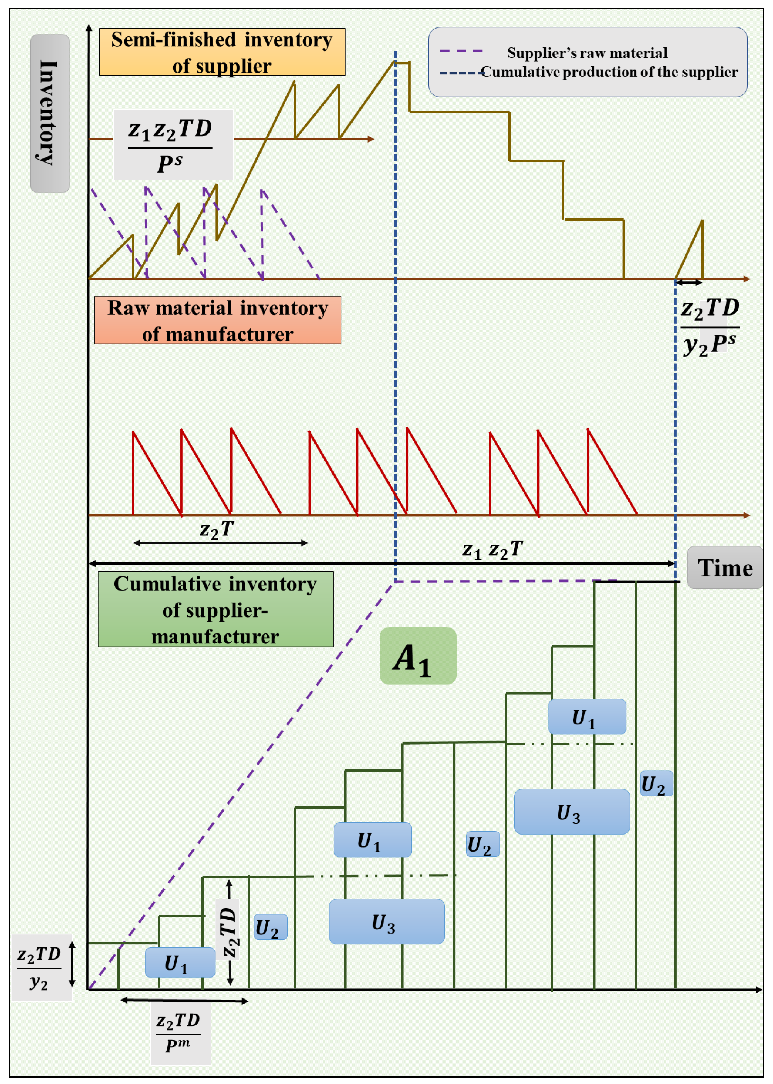
Whereas the supplier receives a total of Q s = z 1 z 2 T D number of raw materials up to time z 1 z 2 T D P s in each cycle of length z 1 z 2 T (see, Figure 2), those items arrive in y 1 number of shipments to be stored in its inventory. Therefore, the average fuzzy holding cost of raw materials for the supplier per unit time ( H C s r ) is as follows:
H C s r = h ¯ r s Q s D 2 P s = D 2 z 1 z 2 T h r s + 1 2 ( δ h r 2 s λ δ h r 1 s λ δ h r 2 s ) 2 y 1 P s .
Holding cost of semifinished products
The supplier stores the semifinished products in its inventory before delivering them to the manufacturer in y 2 shipments within the manufacturer’s cycle ( z 2 T ). Thus, the task is to determine the supplier’s average inventory size of finished products. Accordingly, this study takes a queue from Figure 2 to determine the area A 1 that represents the cumulative production of the supplier as follows (see, for graphical representation, Figure 2, Sarkar et al. [10]):
A 1 = z 2 T 2 2 z 1 2 z 2 T D z 1 2 z 2 T D 2 P s .
Considering A 2 as the average inventory of finished products for the supplier, this study computes the area of a rectangle of type U 1 as follows:
U 1 = z 2 T D y 2 + 2 z 2 T D y 2 + 3 z 2 T D y 2 + + y 2 z 2 T D y 2 z 1 z 2 T D y 2 P m = z 2 T D y 2 1 + 2 + 3 + + y 2 z 1 z 2 T D y 2 P m = z 2 T 2 z 1 z 2 T D 2 ( y 2 + 1 ) y 2 P m .
Likewise, the area of any rectangle of type U 2 is as follows:
U 2 = z 1 z 2 T D z 1 + 2 z 1 z 2 T D z 1 + + z 1 z 1 z 2 T D z 1 z 2 T z 1 z 2 T D z 1 + 2 z 1 z 2 T D z 1 + + z 1 z 1 z 2 T D z 1 z 2 T D P m z 1 z 2 T D P s z 2 T D y 2 = z 1 z 2 T D z 1 ( 1 + 2 + + z 1 ) z 2 T + z 1 z 2 T D z 1 ( 1 + 2 + + z 1 ) z 2 T D P m z 1 z 2 T D P s z 2 T D y 2 = z 2 T 2 z 1 z 2 T ( z 1 + 1 ) D z 1 z 2 T ( z 1 + 1 ) D 2 P m z 1 z 2 T D 2 y 2 P s .
Moreover, this study computes the area of a rectangle of type U 3 as follows:
U 3 = z 2 T D ( 1 + 2 + + ( z 1 1 ) ) z 2 T D P m = z 2 T 2 z 1 z 2 T ( z 1 1 ) D 2 P m .
Therefore, this study measures the area A 2 by taking the aggregate of U 1 , U 2 , and U 3 as follows:
A 2 = z 2 T 2 z 1 z 2 T D 2 ( y 2 + 1 ) y 2 P m + z 1 z 2 T ( z 1 + 1 ) D z 1 z 2 T ( z 1 + 1 ) D 2 P m z 1 z 2 T D 2 y 2 P s + z 1 z 2 T ( z 1 1 ) D 2 P m .
Finally, by subtracting A 2 from A 1 and then dividing the result by the cycle length of the supplier (i.e., z 1 z 2 T ), this study obtains the size of the supplier’s average inventory of finished products A I s as follows:
A I s = z 1 z 2 2 T 2 2 y 2 z 1 D 2 P s + 1 1 y 2 D 2 P m + z 1 1 D .
Hence, this study derives the average fuzzy holding cost of finished products per unit time for the supplier ( H C s f ) as follows:
H C s f = h f s + 1 2 ( δ h f 2 s λ δ h f 1 s λ δ h f 2 s ) 2 A I f s z 1 z 2 T .
Advertisement cost
Under the cooperative advertisement policy (see Section 3.2), the supplier utilizes a fixed part of their advertisement budget to surge the demand of each retailer in any cycle of length z 1 z 2 T . Correspondingly, this study describes the advertisement cost for the supplier per unit time ( A C s ) as follows:
A C s = B A s z 1 z 2 T , where B A s = a s B .
Transportation cost
The supplier bears transportation costs to receive the raw materials in y 1 number of shipments within the supplier’s cycle time z 1 z 2 T . Said per shipment transportation cost has two components, namely variable and fixed components. With Q s = z 1 z 2 T D y 1 as the shipment size of the raw materials to the supplier, this study measures the supplier’s transportation cost per unit time ( T C s ) as follows:
T C s = y 1 F + V Q s z 1 z 2 T .

4.1.2. Cap-and-Trade-Related Cost Components

In addition to fundamental cost components, the supplier addresses the environmental concerns by following the carbon cap-and-trade mechanism of the Paris Accord. This international treaty enforces the supplier to make some annual initial investments to procure modern ecofriendly machinery and associated green technologies.
Green technology investment cost
This study measures the green investment cost for the supplier per unit time ( G T I s ) as follows:
G T I s = G s z 1 z 2 T .
Carbon allowance cost
At the beginning of each year, supplier procures the carbon credits on basis of yearly estimated CEs. Thus, subject to the carbon tax rate δ , this study finds the carbon allowance cost for the supplier per unit time ( C A s ) as follows:
C A s = δ z s z 1 z 2 T .
CE-related setup cost
The setup cost associated with CEs of the supplier in each cycle of length z 1 z 2 T is the product of the carbon tax rate ( δ ) and amount of CEs owing to setup ( B s ), described in per unit time for the supplier ( C E S C s ) as follows:
C E S C s = δ B s z 1 z 2 T .
CE-related production cost
This study describes the CE-related production cost for the supplier in any cycle of length z 1 z 2 T as the product between carbon tax rate ( δ ), weight of CEs for manufacturing ( l s ), and number of semifinished products to be produced in that cycle, illustrated in per unit time for the supplier ( C E P C s ) as follows:
C E P C s = δ l s D .
CE-related holding cost of raw materials
The storage of raw materials in the inventory of the supplier causes CEs up to time z 1 z 2 T D P s in each cycle of length z 1 z 2 T . Here, subject to the average inventory size of those raw materials ( z 1 z 2 T D 2 2 y 1 P s ), this study derives the CE-related holding cost of raw materials for the supplier as a product among the carbon tax rate ( δ ), weight of CE due to holding of raw materials ( c r a w s ), per unit occupied area in inventory ( b r a w s ), and average inventory size, computed in per unit time ( C E H C s r ) as follows:
C E H C s r = δ c r a w s b r a w s z 1 z 2 T D 2 2 y 1 P s .
CE-related holding cost of semifinished products
Likewise, this study determines the CE-related holding cost of semifinished products for the supplier per unit time ( C E H C s f ) as follows:
C E H C s f = δ c s f i n s b s f i n s z 2 T 2 2 y 2 z 1 D 2 P s + 1 1 y 2 D 2 P m + ( z 1 1 ) D .
CE-related environmental impact cost
The emissions of GHGs by the supplier significantly damage the environment. This study computes the CE-related environmental impact cost in each cycle of length z 1 z 2 T as the product of the carbon tax rate ( δ ), environmental impact for inventory ( w s ), and total quantity of semifinished products to be shipped in that cycle. This way, the CE-related environmental impact cost for the supplier per unit time ( C E E I s ) is as follows:
C E E I s = δ w s D .

4.1.3. Total Cost per Unit Time

This way, this study finds the total cost per unit time of the supplier as follows:
T C o s t s = S C s + O C s + P C s + H C s r + H C s f + A C s + T C s + G T I s + 1 ξ 1 exp ( θ G s ) T C E C s C A s ,
where T C E C s = C E S C s + C E P C s + C E H C s r + C E H C s f + C E E I s represents the total CE-related cost of the supplier; the expression T C E C s 1 ξ 1 exp ( θ G s ) symbolizes the supplier’s savings under the carbon cap-and-trade directive. Thus, whenever the relation 1 ξ 1 exp ( θ G s ) T C E C s C A s < 0 holds, the supplier earns additional revenues by selling the surplus carbon credits, if any, in the secondary market within the permissible limits. Again, if 1 ξ 1 exp ( θ G s ) T C E C s C A s > 0 , the supplier has to buy additional carbon credits at higher costs to continue the production operation for the rest of that year.

4.2. Various Cost Components of the Manufacturer

This subsection deliberates on various cost components of the manufacturer as follows:

4.2.1. Fundamental Cost Components

Setup cost
This study considers the fuzzy setup cost ( a ˜ m ) to be associated with the establishment of the business by the manufacturer in each cycle of length z 2 T , derived in per unit time ( S C m ) as follows:
S C m = a m + 1 2 ( δ a 2 m λ δ a 1 m λ δ a 2 m ) z 2 T .
Ordering cost
The manufacturer places the order to receive the semifinished products in y 2 number of shipments in any cycle of length z 2 T . As a result, the fuzzy ordering cost per unit time ( O C m ) is as follows:
O C m = y 2 o m + 1 2 ( δ o 2 m λ δ o 1 m λ δ o 2 m ) z 2 T .
Production cost
This study considers the remanufacturing of the faulty products with fresh raw materials by incurring additional labor- and energy-related costs at the manufacturer in any cycle of length z 2 T . Thus, likewise to relation (8), this study determines the production cost for the manufacturer per unit time ( P C m ( P m ) ) as follows:
P C m = c ¯ 0 m + c d c m P m + α m P m P m + c ¯ d m + ω m c ¯ 0 m β m exp ( η m z 2 T ) P m .
Holding cost of semifinished products
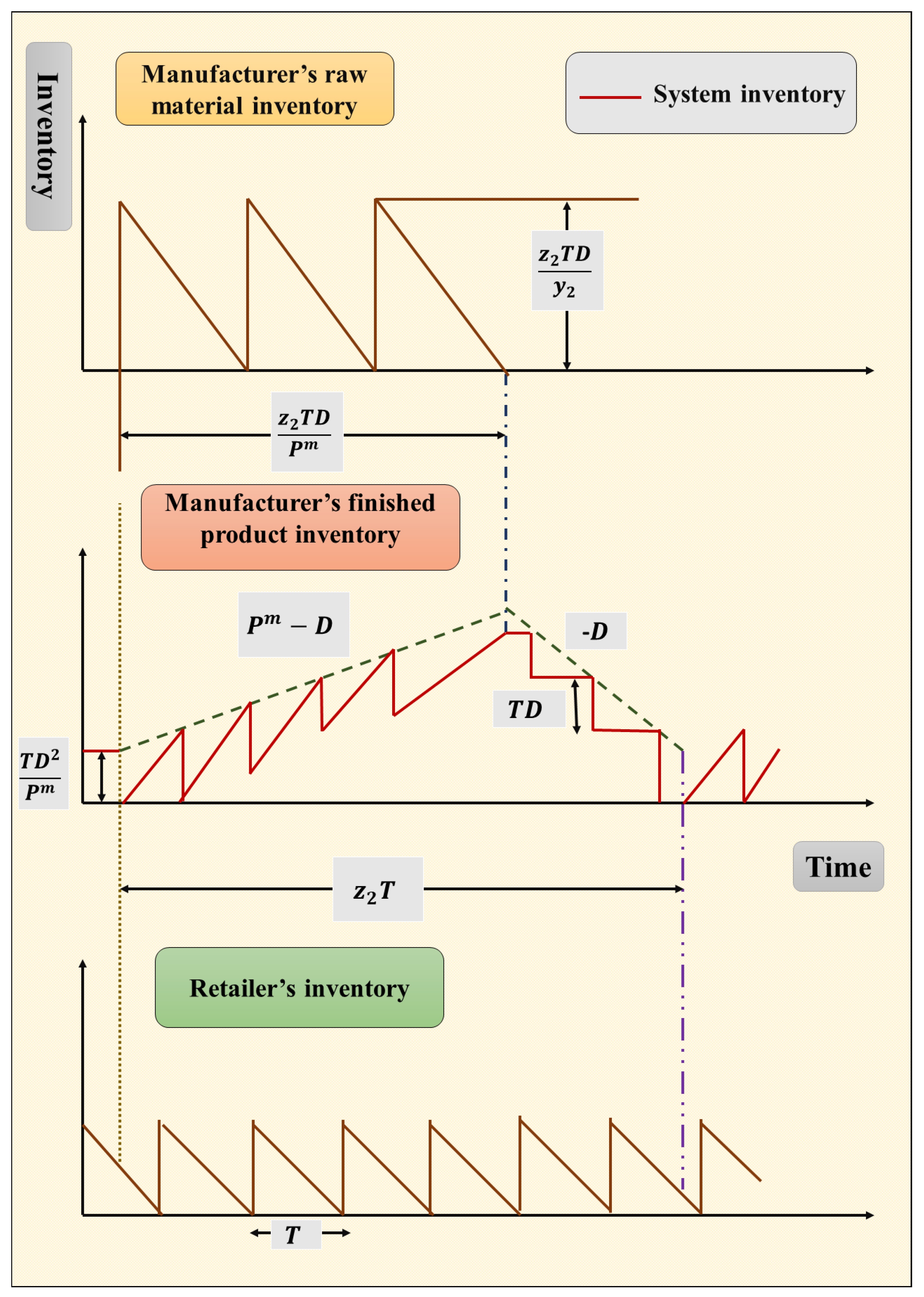
The manufacturer stores the semifinished products in the inventory by procuring those Q m ( = z 2 T D ) items in y 2 number of shipments up to time z 2 T D P m in any cycle of length z 2 T . Accordingly, this study divides the triangular area signifying the inventory of raw materials for the manufacturer in Figure 3 by z 2 T , yielding the average fuzzy holding cost of semifinished products per unit time for the manufacturer ( H C m r ) as follows:
H C m r = h ¯ r m Q m D 2 P m = h r m + 1 2 ( δ h r 2 m λ δ h r 1 m λ δ h r 2 m ) 2 P m y 2 z 2 T D 2 .
Holding cost of finished products
The stack of finished products in the manufacturer’s inventory occupies some space, thus incurring some holding costs for the manufacturer. In the beginning, the manufacturer’s inventory level is zero, while retailers start with a total of T D 2 P m units of products. Furthermore, each retailer receives the finished products from the manufacturer in z 2 shipments of equal size. The inventory level of the manufacturer is set to increase at the rate ( P m D ) , thus providing the maximum combined inventory level of the manufacturer–retailers system as follows (for graphical illustration, see Figure 3):
( P m D ) z 2 T D P m + T D 2 P m .
After that, because the manufacturer fulfills the orders to be placed by different retailers at the rate D, its inventory level decreases in line. This way, the following expression governs the average combined inventory level of that system:
( P m D ) z 2 T D 2 P m + T D 2 P m .
This yields the aggregate of the average inventory in each shipment across retailers as follows:
( P m D ) z 2 T D z 2 P m + T D 2 P m T D 2 , i . e . , T D 2 .
Therefore, one obtains the size of the manufacturer’s average inventory by subtracting the inventory for all retailers from the average combined inventory level of the aforementioned system as follows:
A I m f = ( P m D ) z 2 T D 2 P m + T D 2 P m T D 2 = T 2 ( 2 z 2 ) D 2 P m + ( z 2 1 ) D .
Thus, this study outlines the average fuzzy holding cost of finished products for the manufacturer per unit time ( H C m f ) as follows:
H C m f = h ¯ f m A I m f = h f m + 1 2 ( δ h f 2 m λ δ h f 1 m λ δ h f 2 m ) 2 T ( 2 z 2 ) D 2 P m + ( z 2 1 ) D .
Advertisement cost
This study takes the cooperative advertising cost for the manufacturer per unit time ( A C m ) as follows:
A C m = B A m z 2 T .
Transportation cost
This study considers the transportation cost per unit time for the manufacturer ( T C m ) as follows:
T C m = y 2 F + V Q m z 2 T .

4.2.2. Cap-and-Trade-Related Cost Components

This study considers the various cost components to be associated with the carbon cap-and-trade mechanism of the Paris Accord for the manufacturer as follows:
Green technology investment cost
In order to be ecofriendly, and thus, sustainable, the manufacturer makes annual green-technology-related investments to accept the carbon cap-and-trade mechanism of the Paris Accord in each cycle of length z 2 T , outlined in per unit time ( G T I m ) as follows:
G T I m = G m z 2 T .
Carbon allowance cost
The manufacturer procures the carbon credits on the basis of estimated yearly CEs in each cycle of length z 2 T , correspondingly providing the carbon allowance cost per unit time ( C A m ) as follows:
C A m = δ z m z 2 T .
CE-related setup cost
In each cycle of length z 2 T , the manufacturer bears the setup cost associated with CEs per unit time ( C E S C m ) as follows:
C E S C m = δ B m z 2 T .
CE-related production cost
This study describes the CE-related production cost for the manufacturer in any cycle of length z 2 T as the product between carbon tax rate ( δ ), weight of CE for manufacturing ( l m ), and number of semifinished products to be produced by the manufacturer in that cycle. Thus, this study determines the CE-related production cost for the manufacturer per unit time ( C E P C m ) as follows:
C E P C m = δ l m D .
CE-related holding cost of semifinished items
The holding of semifinished products in the inventory of the manufacturer results in CEs in any cycle of length z 2 T , illustrated in per unit time ( C E H C m r ) as follows:
C E H C m r = δ c s f i n m b s f i n m z 2 T D 2 2 P m y 2 .
CE-related holding cost of finished products
Moreover, subject to the required space per unit product ( b f i n m ), CEs per unit area ( c f i n m ), and carbon tax rate ( δ ), this study elaborates the CE-related holding cost of finished products for the manufacturer per unit time ( C E H C m f ) as follows:
C E H C m f = δ c f i n m b f i n m T 2 ( 2 z 2 ) D 2 P m + ( z 2 1 ) D .
CE-related environmental impact cost
This study reports the CE-related environmental impact cost per unit time for the manufacturer ( C E E I m ) as follows:
C E E I m = δ w m D .

4.2.3. Total Cost per Unit Time

This way, this study finds the total cost per unit time for the manufacturer as follows:
T C o s t m = S C m + O C m + P C m + H C m r + H C m f + A C m + T C m + G T I m + 1 ξ 1 exp ( θ G m ) T C E C m C A m ,
where T C E C m = C E S C m + C E P C m + C E H C m r + C E H C m f + C E E I m is the CE-related total cost for the manufacturer. Under the carbon cap-and-trade mechanism of the Paris Accord, this study computes the potential savings of the manufacturer as T C E C m ( 1 ξ ( 1 exp ( θ G m ) ) ) . In case 1 ξ 1 exp ( θ G m ) T C E C m C A m < 0 , the manufacturer earns additional revenues by selling any unused carbon credits in secondary markets, while for 1 ξ 1 exp ( θ G m ) T C E C m C A m > 0 , the manufacturer procures the additional carbon credits from secondary markets to carry on the regular production operation.

4.3. Various Cost Components of Any ith Retailer

The present study considers that the k retailers, which are spread across different locations, procure the finished products from a single manufacturer on the basis of the prevailing demand from respective customers. This subsection deliberates on various cost components for the ith retailer as follows:

4.3.1. Fundamental Cost Components

Setup cost
In each cycle of length T, the i th ,   i = 1 , , k retailer incurs a one-time fuzzy setup cost, outlined in per unit time ( S C i r ) as follows:
S C i r = a i r + 1 2 ( δ a i 2 r λ δ a i 1 r λ δ a i 2 r ) T .
Ordering cost
The i th ,   i = 1 , , k retailer incurs the fuzzy ordering cost to be associated with the ordering, packaging, shipping, etc., of deliverables per unit time ( O C i r ) as follows:
O C i r = o i r + 1 2 δ o i 2 r λ δ o i 1 r λ δ o i 2 r T .
Holding cost
Any i th ,   i = 1 , , k retailer receives the finished products from the manufacturer at the beginning of each cycle and stores those in its inventory. Thus, the i th ,   i = 1 , , k retailer pays the holding cost per unit time ( H C i r ) as follows (for graphical illustration, see Figure 3):
H C i r = T d i h i r + 1 2 ( δ h i 2 r λ δ h i 1 r λ δ h i 2 r ) 2 .
Advertisement cost
The i th ,   i = 1 , , k retailer bears a part of the promotional-activities-related total expenses under the cooperative advertisement policy of the proposed model, derived in per unit time ( A C i r ) as follows:
A C i r = b i r T .

4.3.2. Cap-and-Trade-Related Cost Components

Green technology investment cost
In addition to the supplier and the manufacturer, the present study finds that each retailer abides by the carbon cap-and-trade mechanism of the Paris Accord. Thus, this procures modern ecofriendly machinery, along with recent technologies, at the beginning of each cycle of length T, described in per unit time ( G T I i r ) as follows:
G T I i r = G i r T .
Carbon allowance cost
At the beginning of each cycle of length T, the i th ,   i = 1 , , k retailer secures an estimated CE quota to follow the carbon cap-and-trade directive of the Paris Accord, obtained in per unit time ( C A i r ) as follows:
C A i r = δ z i r T .
CE-related setup cost
The present study computes the CE-associated setup cost for i th ,   i = 1 , , k retailer per unit time ( C E S C i r ) as follows:
C E S C i r = δ B i r T .
CE-related holding cost
In each cycle of length T, the storage of finished products in the inventory of i th ,   i = 1 , , k retailer prior to their sale calls for the CE-related average fuzzy holding cost per unit time ( C E H C i r ) as follows:
C E H C i r = δ c f i n i r b f i n i r d i 2 .
CE-related environmental impact cost
Various organizational activities of the i th ,   i = 1 , , k retailer cause the environmental degradation in each cycle of length T, determined in per unit time ( C E E I i r ) as follows:
C E E I i r = δ w r d i .

4.3.3. Total Cost per Unit Time

This way, this study finds the total cost per unit time of the ith retailer as follows:
T C o s t i r = S C i r + O C i r + H C i r + A C i r + G T I i r + 1 ξ 1 exp ( θ G i r ) T C i E C r C A i r ,
where T C i E C r = C E S C i r + C E H C i r + C E E I i r is the CE-related total cost of the ith retailer. As before, the potential savings of the retailer are T C i E C r 1 ξ 1 exp ( θ G i r ) . The ith retailer earns additional revenues by selling any unused carbon credits in secondary markets, provided 1 ξ 1 exp ( θ G i r ) T C i E C r C A i r < 0 . However, in case ( 1 ξ ( 1 exp ( θ G i r ) ) ) T C i E C r C A i r > 0 , the retailer procures the additional carbon credits from secondary markets to carry on the regular production operation.

4.4. Net Profit per Unit Time of the Proposed SSCM Model

A number of articles deliberate on the direct relationships between the per unit sale price of finished products and the maximum advertisement budget, beyond which business turns enviable. Accordingly, this study considers the revenue of the ith retailer of the proposed model as R e v i ( B , T ) = ( α + β B d i ) T . Thus, this study describes the aggregate revenue per unit time of the proposed SSCM model ( T R S S C M ) as follows:
T R S S C M = i = 1 k α + β B d i = α + β B D .
By considering the various cost components of all chain partners, this study formulates the net profit per unit time of the proposed SSCM model ( N P S S C M ) as follows (For detailed components, see (A42)):
N P S S C M = T R S S C M T C o s t s + T C o s t m + i = 1 k T C o s t i r .
This study aims to determine the optimal cycle length (T), aggregate advertisement budget (B), GTI ( G s , G m , G r ), and production rates ( P s , P m ) of various chain partners, which, in turn, can improve the profitability of the proposed SSCM model.

5. Solution Methodology

This section analyzes the proposed net profit per unit time to correspondingly formulate one optimization model. Then, this derives an algorithm illustrating the solution methodology of that model. Later, this study extracts some analytical insights.

5.1. Towards Global Optimality

With the aim to maximize the profitability of the proposed SC (see, relation (57)), this study formulates one optimization-based mathematical model. Owing to the consideration of three integer-type decision variables, namely G s , G m , and G r , and four other continuous-type decision variables, namely P s , P m , B , and T , the following mathematical model is regarded as a mixed-integer nonlinear programming model:
max N P S S C M ( G s , G m , G r , P s , P m , B , T ) subject to G s , G m , G r N , B , T , P s , P m 0 .
Among numerous existing optimization approaches establishing the global optimality of N P S S C M of the model (58), this study opts for the classical optimization method, which efficiently determines the optimum solutions of any continuous and differentiable function. Moreover, this well-established method is analytical in nature, and makes use of tools from differential calculus to locate the maximum and minimum points for unconstrained and constrained continuous objective functions.
In this regard, this study firstly determines a critical point A * ( P s * , P m * , B * , T * ) by solving four simultaneous equations that are derived by equating four first-order partial derivatives of N P S S C M with respect to P s , P m , B , and T respectively, to zero (see, for derivatives, Appendix B). Components of the aforementioned critical point A * are as follows:
i . 2 α s P s 3 + c ¯ 0 s + c ¯ d s + c ¯ 0 s ω s β s exp ( η s z 1 z 2 T ) P s 2 D 2 z 1 z 2 T h ¯ r s 2 y 1 h ¯ f s z 2 T 2 y 2 z 1 D 2 2 1 ξ ( 1 exp ( θ G s ) ) δ c r a w s b r a w s z 1 z 2 T D 2 2 y 1 + δ c s f i n s b s f i n s z 2 T ( 2 y 2 z 1 ) D 2 2 = 0 , i . e . , P s * = ϕ s ( P s * ) + constant .
i i . 2 α m P m 3 + c ¯ 0 m + c ¯ d m + c ¯ 0 m ω m β m exp ( η m z 2 T ) P m 2 h ¯ f m T ( 2 z 2 ) D 2 2 h ¯ f s z 2 T 1 1 y 2 D 2 2 z 2 T D 2 h ¯ r m 2 y 2 ( 1 ξ ( 1 exp ( θ G s ) ) ) δ c s f i n s b s f i n s z 2 T 1 1 y 2 D 2 2 ( 1 ξ ( 1 exp ( θ G m ) ) ) δ c s f i n m b s f i n m z 2 T D 2 2 y 2 + δ c f i n m b f i n m T ( 2 z 2 ) D 2 2 = 0 , i . e . , P m * = ϕ m ( P m * ) + constant .
i i i . a r T + β D 2 B a s z 1 z 2 T a m z 2 T = 0 , i . e . , B * = β D z 1 z 2 T 2 a r z 1 z 2 + a m z 1 + a s 2 .
i v . G s z 1 z 2 T 2 ( 1 ξ ( 1 exp ( θ G r ) ) ) δ B r T 2 + δ z r T 2 + G r T 2 + a ¯ r T 2 + o ¯ r T 2 h ¯ f m ( 2 z 2 ) D 2 P m + ( z 2 1 ) D 2 + y 2 o ¯ m z 2 T 2 + y 1 o ¯ s z 1 z 2 T 2 + y 2 F z 2 T 2 + a ¯ s z 1 z 2 T 2 + a ¯ m z 2 T 2 h ¯ r D 2 z 2 D 2 h ¯ r m 2 y 2 P m D 2 z 1 z 2 h ¯ r s 2 y 1 P s + a s B z 1 z 2 T 2 h ¯ f s z 2 2 ( 2 y 2 z 1 ) D 2 P s + ( 1 1 y 2 ) D 2 P m + ( z 1 1 ) D + δ c s f i n s b s f i n s z 2 2 y 2 z 1 D 2 P s 2 + 1 1 y 2 D 2 P m + z 2 1 D 2 ( 1 ξ ( 1 exp ( θ G s ) ) ) δ B s z 1 z 2 T 2 + δ c r a w s b r a w s z 1 z 2 D 2 2 y 1 P s + δ z s z 1 z 2 T 2 + G m z 2 T 2 + a m B z 2 T 2 + a r B T 2 + y 1 F z 1 z 2 T 2 ( 1 ξ ( 1 exp ( θ G m ) ) ) δ B m z 2 T 2 + δ c s f i n m b s f i n m z 2 D 2 2 y 2 P m + δ c f i n m b f i n m ( 2 z 2 ) D 2 P m + ( z 2 1 ) D 2 + δ z m z 2 T 2 c ¯ d s + c ¯ 0 s ω s η s z 1 z 2 β s exp ( η s z 1 z 2 T ) P s c ¯ d m + c ¯ 0 m ω m η m z 2 β m exp ( η m z 2 T ) P m = 0 , i . e . , T * = constant ϕ T ( T * ) + c ¯ d s + c ¯ 0 s ω s η s z 1 z 2 β s exp ( η s z 1 z 2 T * ) P s + c ¯ d m + c ¯ 0 m ω m η m z 2 β m exp ( η m z 2 T * ) P m .
Thereafter, the following theorem determines the conditions for the concavity of N P S S C M with respect to the continuous decision variables P s , P m , B , T :
Theorem 1.
Considering any discrete green investments of various chain partners, the net profit per unit time of the proposed SSCM model is concave at the critical point A * ( P s * , P m * , B * , T * ) with respect to:
i .   P s (supplier’s production rate), provided y 2 z 1 2 ;
i i .   P m (manufacturer’s production rate), provided z 2 2 ;
i i i .   T (ith retailer’s cycle length), provided B τ 1 z τ 1 , τ 1 = s , m , r ; and
i v .   B (aggregate advertisement budget).
Proof. 
See Appendix B. □
Next, the following theorem sufficiently determines the criteria to attain the global maximum for N P S S C M at A * .
Theorem 2.
For any discrete green investments of chain partners, the net profit per unit time of the proposed SSCM model is the global maximum at the critically determined production rates, advertisement budget, and retailer’s cycle length, subject to the following condition:
F > m a x 2 E 3 2 E 1 E 2 z 1 z 2 T 2 E 1 y 2 z 1 + y 1 , 4 E 7 2 E 6 E 2 z 1 z 2 T y 2 z 1 + y 1 E 6 , 4 E 4 2 E 5 E 2 z 1 z 2 T y 2 z 1 + y 1 E 5 .
Proof. 
See Appendix C. □
Regarding the optimality of N P S S C M with respect to G s , G m , and G r , this study considers N P S S C M at the critical point A * ( P s * , P m * , B * , T * ) , thereby framing the following theorem:
Theorem 3.
The net profit per unit time of the proposed SSCM model satisfies the following inequalities:
τ : G s * , G m * , G r * : N P S S C M ( τ 1 ) N P S S C M ( τ ) and N P S S C M ( τ ) N P S S C M ( τ + 1 ) ,
at the critical point A * , provided as follows:
i . 1 θ log ξ E 19 exp ( θ ) 1 z 1 z 2 T * 1 G s * 1 θ log ξ E 19 exp ( θ ) 1 z 1 z 2 T * , i i . 1 θ log ξ E 20 exp ( θ ) 1 z 2 T * 1 G m * 1 θ log ξ E 20 exp ( θ ) 1 z 2 T * , and i i i . 1 θ log ξ E 21 exp ( θ ) 1 T * 1 G r * 1 θ log ξ E 21 exp ( θ ) 1 T * ,
from which N P S S C M takes the following form:
N P S S C M = N P S S C M ( G s * , A * ) , for fixed G m , G r , N P S S C M ( G m * , A * ) , for fixed G s , G r , N P S S C M ( G r * , A * ) , for fixed G s , G m .
Proof. 
See Appendix D. □
This way, the current study redesigns the model (4), and thus defines the following optimization problem:
max N P S S C M ( G s , G m , G r , P s , P m , B , T ) subject to y 2 z 1 2 , z 2 2 , z τ 1 B τ 1 , τ 1 = s , m , r , F > m a x 2 E 3 2 E 1 E 2 z 1 z 2 T 2 E 1 y 2 z 1 + y 1 , 4 E 7 2 E 6 E 2 z 1 z 2 T y 2 z 1 + y 1 E 6 , 4 E 4 2 E 5 E 2 z 1 z 2 T y 2 z 1 + y 1 E 5 , 1 θ log ξ E 19 exp ( θ ) 1 z 1 z 2 T * 1 G s * 1 θ log ξ E 19 exp ( θ ) 1 z 1 z 2 T * , 1 θ log ξ E 20 exp ( θ ) 1 z 2 T * 1 G m * 1 θ log ξ E 20 exp ( θ ) 1 z 2 T * , 1 θ log ξ E 21 exp ( θ ) 1 T * 1 G r * 1 θ log ξ E 21 exp ( θ ) 1 T * G s , G m , G r N , B , T , P s , P m 0 .
The solution of this model exhibits the global optimality of the net profit of the proposed SSCM model.

5.2. Algorithm

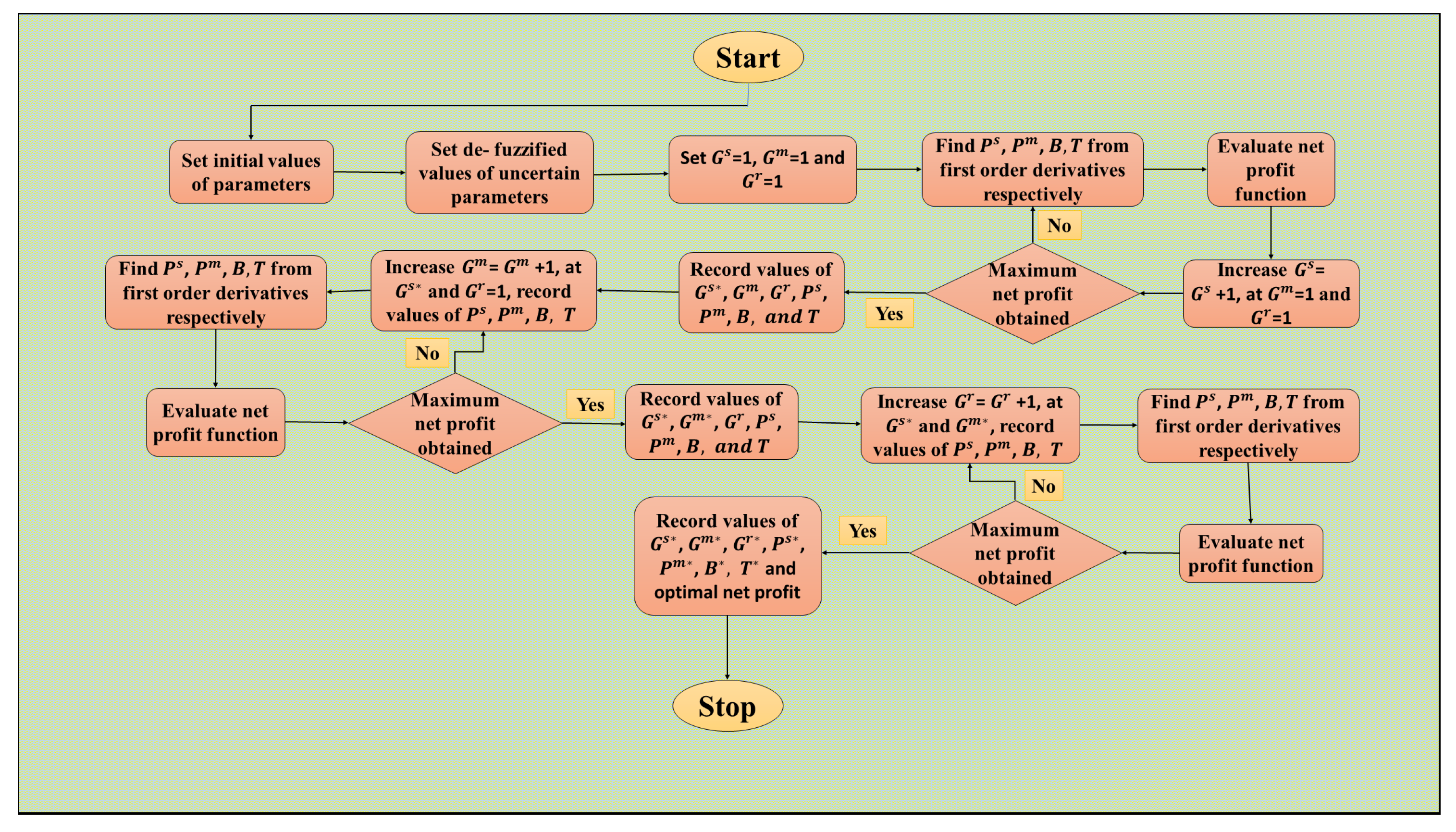
All these derivations lead the present study to frame an optimization algorithm, to be called the KGM algorithm on basis of the family names of the authors, to find out the optimal solutions for any fuzzy mixed-integer nonlinear programming problems. In this regard, Figure 4 graphically describes the various steps of the proposed algorithm.

5.3. Wide-Ranging Demand Rate and Various Decisions of the Proposed Model

A change in demand refers to a change in consumer preference for buying a specific good or service. Organizations have a lot of concerns about this wide-ranging demand rate from customers. Thus, this seems essential to explore the relationships connecting the demand rates across retailers with various decisions of the proposed model as follows:
  • Revenue and total cost
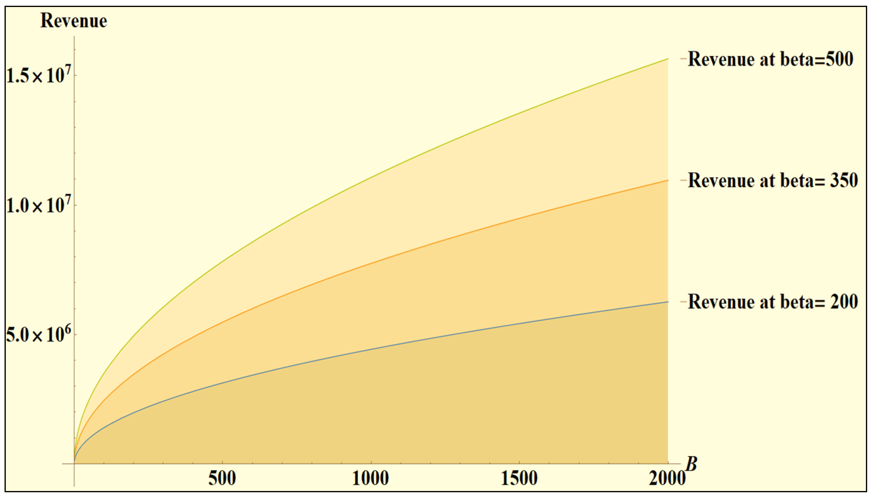
This study finds that an uncontrollable hike in demand rate is unwanted for the managers. Post a certain demand level, the business turns into a loss, while a systematic hike in demand rate improves its revenue (see, Figure 5).
  • Cycle lengths of various chain partners
Constraints y 2 z 1 2 and z 2 2 of the proposed optimization model (66) seek the same cycle length for both the supplier and manufacturer. Moreover, this implies that two shipments of products in each cycle are to be procured by the manufacturer. Again, regarding the relation between ith retailer’s cycle length and demand rate across retailers, this study obtains the following relation:
ν 0 D 2 + ν 22 D + ψ ( T ) = 0 .
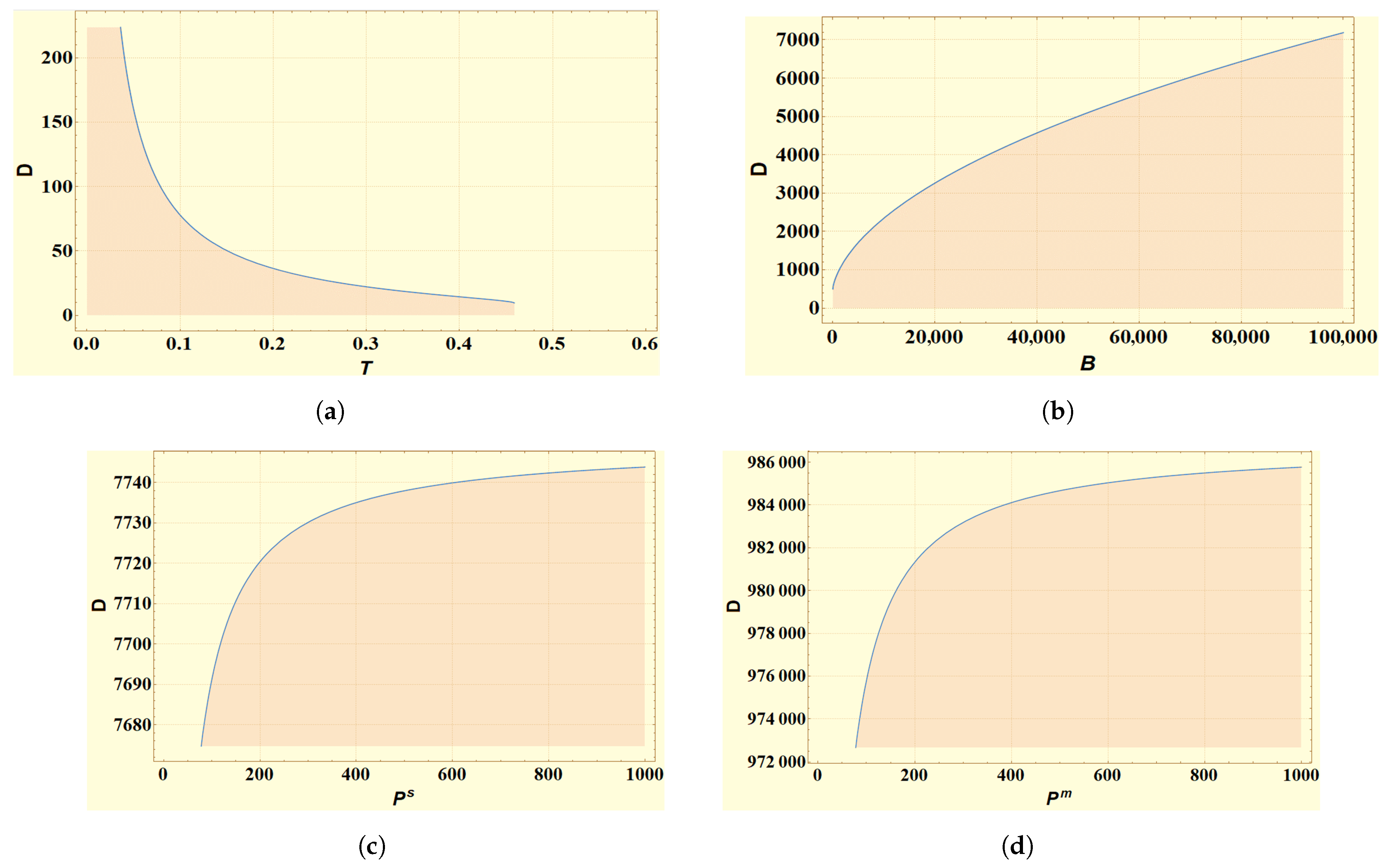
As graphically illustrated in Figure 6a, this study finds that whenever the demand rate across retailers is fragile, retailers (and other chain partners) need to take some longer cycles. However, in case the retailers’ demand rate increases significantly, they should gradually reduce the cycle length.
  • Supplier’s and manufacturer’s production rates
The following relations connect the demand rate across retailers with the production rates of the supplier and manufacturer, respectively (for notations, see Appendix E):
ν 1 P s + ν 2 D 2 + ν 3 D + ν 4 P s 2 + ν 5 P s + ν 6 = 0 ,
ν 7 P m + ν 8 D 2 + ν 9 D + ν 10 P m 2 + ν 11 P m + ν 12 = 0 .
Figure 6c,d depict the results graphically. Accordingly, the production rates of the supplier and manufacturer increase with each upsurge in the demand rate at retailers. However, each increase in retailers’ demand rate causes the growth rates for both production rates to gradually slow down.
  • Aggregate advertisement budget
This study determines the following relation between retailers’ demand rate and aggregate advertisement budget:
ν 18 D 2 + ν 19 D + β D B + ν 20 B + ν 21 = 0 .
Relation (70) and Figure 6b implore the SC management to increase the aggregate advertising expenditure in order to strengthen the retailers’ shaky demand rate. Any additional investment in advertising can still scarcely result in the same growth rate for demand when the shops already have a sizable rate of demand. In the same way, if the current advertising budget is barely a fair amount, this study suggests significantly raising the overall advertising budget in order to quickly boost the earning of the suggested SSCM model (see Figure 7). This is more relevant for higher values of the parameter β .

6. Numerical Experiments

This section numerically validates the applicability of the proposed SSCM model. In this regard, firstly, this study experiments with one example, in which the data are extracted from several well-established articles and then modified according to the current elaboration. Next, this study considers one real-life-based case study related to the extraction of crude oil from any underground reservoirs and ocean beds (i.e., the supplier), the subsequent processing of it in oil refineries (i.e., the manufacturer), and then its sale to customers through retailers. Worldwide, large organizations, such as Saudi Aramco, PetroChina, TotalEnergies, and IndianOil, are leaders in this sector.
In both, this study considers the fluctuations in market conditions that are well represented through varying values of the degree-of-optimism-related parameter λ . Accordingly, three different values of λ , namely λ = 1 for the bullish market, λ = 0.5 for the stable market, and λ = 0.5 for the bearish market, are taken. Moreover, all of the results are computed in M A T L A B R 2022 B software on a desktop computer with I n t e l ® C O R E T M i 7 processor, 64 GB in RAM, and Windows 10 ® operating system.

6.1. Experiment I

In this experiment, this study takes the data from two well-established articles, namely Sarkar et al. [10] and Mishra et al. [6], into account. While Table 3 enlists the values of various crisp parameters, Table 4 displays the values of all fuzzy parameters.

6.1.1. Results

Table 5 displays the optimal results. In comparison to bearish and stable market conditions, the net profit per unit time of the proposed SSCM model in a bullish market increases by 0.49 % and 0.24 % , respectively, whereas the consistency of the overall advertising budget in every market scenario gives the model endurance in choppy market situations. Every time the market conditions improve, the unit net profit gets maximized by slowing the supplier’s and manufacturer’s production rates and taking the slightly longer cycle length of the retailer into account. Interestingly, slowing down production and extending the cycle time creates a perception of scarcity or exclusivity, potentially driving up demand and allowing for higher prices, leading to increased net profit. However, this is vital to take the specific market dynamics and customer preferences into account.
Again, in bullish and stable market conditions, respectively, there is a 0.92 % and 0.27 % deceleration in the supplier’s production rate compared to the bearish market conditions. Taking into account the same for the manufacturer, 10.14 % and 4.24 % of deceleration along with 16.05 % and 5.14 % longer cycle lengths are found to be optimal for various retailers in bullish and stable market conditions, respectively, with the same comparison in bearish market conditions. Last but not least, the annual GTI stability at each chain partner shows the consistency of the proposed model. Additional investigations with a real-life data-oriented case study justify the current findings.

6.1.2. Sensitivity Analysis

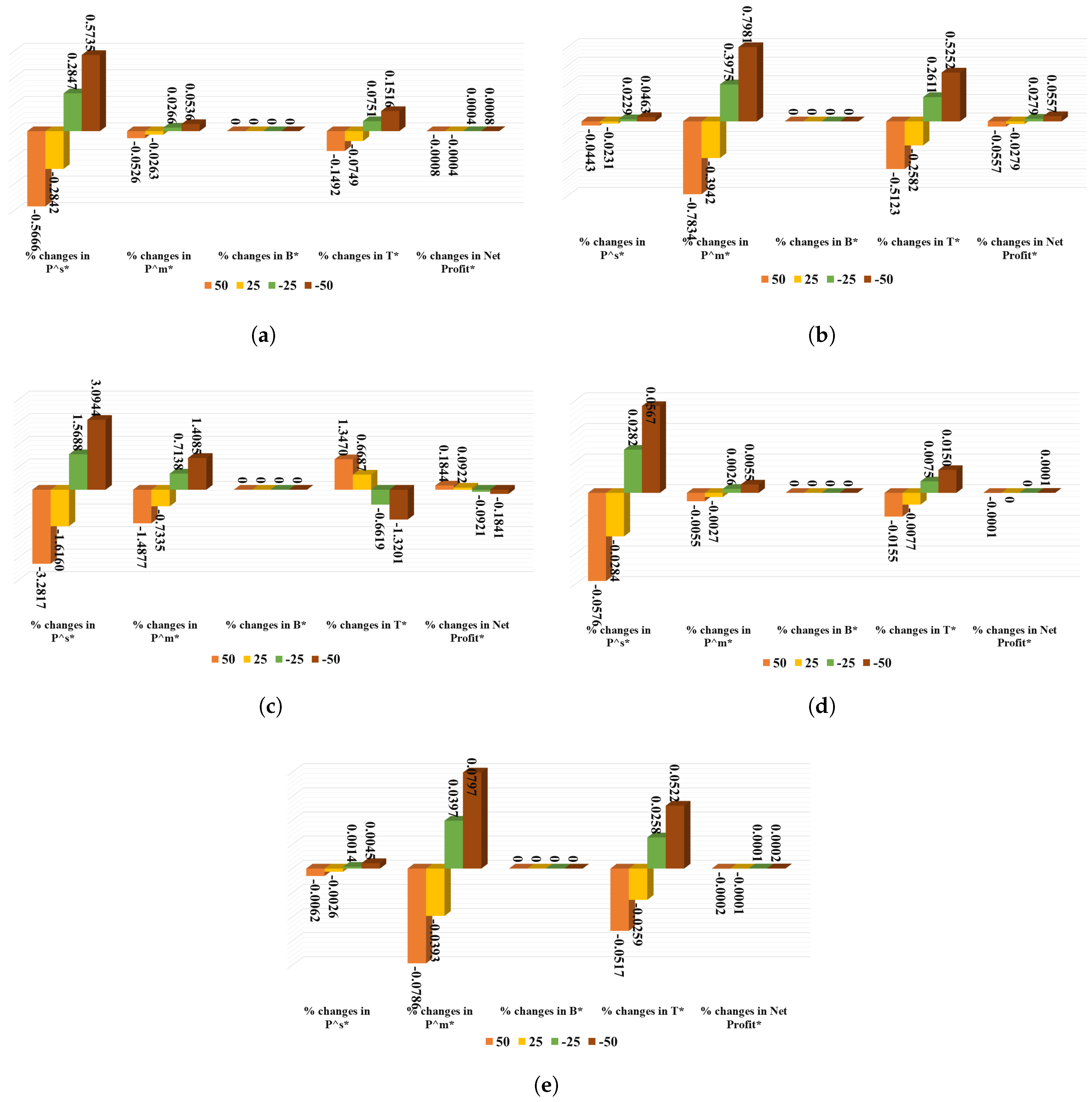
This subsection assesses the changes in the maximum net profit per unit time ( N P S S C M * ) along with the corresponding optimal values of all continuous-type decision variables, such as the production rate of the supplier ( P s * ) and the manufacturer ( P m * ), the aggregate advertisement budget ( B * ), and the cycle length of retailers ( T * ), under the amendments of few major parameters, such as the defuzzified reworking cost of defective items of the supplier ( c ¯ d s ) and the manufacturer ( c ¯ d m ), the remanufacturing of related additional raw materials by the supplier ( ω s ) and the manufacturer ( ω m ), and the fraction of CE reduction ( ξ ) after green investment in the bullish market. This study successively modifies the initial values of those parameters by 50 % , 25 % , 25 % , and 50 % , while fetching one parameter at a time, and with all other parameters remaining fixed at base values to observe as follows:
  • This study finds the optimal aggregate advertisement budget ( B * ) to be insensitive to any changes in values of any aforementioned parameters.
  • Due to any changes in the parameter c ¯ d s , the current results indicate an insensitive net profit per unit of time. While the production rate of the supplier ( P s * ) is modestly sensitive, the same for the manufacturer ( P m * ) is slightly sensitive with respect to all changes in values of c ¯ d s . The retailer’s cycle length T * consistently shortens with systematic increases in c ¯ d s (see Figure 8a).
  • Subject to various changes in values of c ¯ d m (see Table 6), the current analysis finds the manufacturer’s production rate ( P m * ) and the retailers’ cycle length ( T * ) to be moderately sensitive, while net profit per unit time and the supplier’s production rate ( P s * ) are lowly sensitive. Figure 8b displays these results.
  • Changes in the values of the parameter ξ cause proportionate changes in the manufacturer’s production rate ( P m * ) and retailers’ cycle length ( T * ) . Nevertheless, the profitability of the proposed model is modestly correlative to the changes in values of ξ , while the supplier’s production rate ( P s * ) is highly sensitive to those changes. One can explore Figure 8c in this regard.
  • Net profit per unit time of the proposed model is hardly changed owing to any changes in values of ω s and ω m . Except for the barely sensitive cycle length of retailers for the moderate changes in values of ω s , this study finds the retailers’ cycle length to be lowly sensitive to any changes in values of both ω s and ω m . However, P s * and P m * are lowly sensitive with respect to any changes in values of ω s and ω m , respectively, while turning insensitive in other cases (see Figure 8d,e for details).

6.1.3. Insights

The present study extracts a number of meaningful managerial insights for the future consideration of SC managers on the basis of the results in Section 6.1.2 as follows:
  • Observations: Any drops in remanufacturing-related labor and energy costs for the supplier and manufacturer correspondingly cause moderately higher production rates therein, while adequately prolonging the cycle length and improving profitability to a certain extent. On the other hand, when a firm (i.e., the supplier/manufacturer) utilizes fewer fresh materials during remanufacturing, there are some opportunities left to increase the production rate therein and to prolong the cycle length a little.
    Recommendations: SC managers should follow some best practices, including lean manufacturing principles, to improve profitability in a manufacturing–remanufacturing context. These policies focus on reducing waste and increasing efficiency throughout the manufacturing process. Moreover, lean manufacturing necessitates streamlined processes, improved quality control, and reduced inventory levels. When a firm utilizes fewer fresh materials during remanufacturing, there lie opportunities to increase production rates and prolong the cycle length. This involves exploring alternative raw materials, reconfiguring production processes, or investing in new technologies.
    Moreover, since the landscape related to the immediate remanufacturing of faulty products is constantly evolving, automation can reduce labor costs and improve production rates. While the upfront costs of automation can be significant, over the long term, this can lead to significant cost savings and improved efficiency for various chain partners. Ultimately, SC managers should be proactive in identifying opportunities to improve efficiency and profitability throughout the manufacturing process. By working closely with suppliers and manufacturers, monitoring costs and performance metrics, and continuously seeking ways to optimize the supply chain, they can help to drive success and growth for their organizations.
  • Observations: Increased values of the GTI-induced CE reduction rate proportionately improve the net profit per unit time, considerably reduce the production rates at both supplier and manufacturer, and give prolonged cycle length to various chain partners.
    Recommendations: SC managers should consider implementing technology solutions to reduce CEs, such as energy-efficient machinery, green energy sources, and data-driven optimization tools. These solutions can help to improve efficiency and reduce emissions, while also increasing profitability. Overall, a comprehensive and collaborative approach is needed to implement green investment and increase the carbon emission reduction rate effectively. By working closely with supply chain partners, leveraging technology solutions, and continuously monitoring and adjusting the strategy, managers can achieve both environmental and financial goals.

6.2. Experiment II: Case Study

The majority of the world’s energy comes from oil, and every day, oil corporations supply billions of barrels of petroleum products to industry and transportation. Measures to cut back on the use of carbon-based fuels and growing public concern about climate change have not yet had a significant influence on the business. In this context, this study takes the extraction of crude oil from any underground reservoirs and ocean beds (i.e., suppliers) and subsequent processing of it in oil refineries (i.e., manufacturers) into account. Organizations process crude oil and refine it into more valuable products (e.g., petroleum, naphtha, petrol, diesel, kerosene, liquefied petroleum gas, and jet fuel). These items are then transferred from any refinery to numerous fuel stations and other retail points. Contrary to popular belief, this sector occasionally experiences market uncertainty that impacts a number of cost components of various chain partners.
These business requirements make it fit the majority of the data used in this study (for crisp parameters, see Table 7), depicting that all these occurrences come from well-established articles, such as Rout et al. [25] and Sepehri et al. [46], while the degree of optimism (i.e., λ ), as associated with several asymmetric TFN-type parameters, takes varied values, reflecting the uncertainty in the market (for fuzzy parameters, see Table 8).

6.2.1. Results

Table 9 exhibits the optimal outcomes, based on which this study argues the following:
The maximum net profit per unit time of the proposed SSCM model in a bullish market is 1.03 % and 0.52 % more than those in bearish and stable markets, respectively. Thus, the profitability of the proposed model improves with each revival in the market condition.
When it comes to CE reduction, different chain partners, in particular retailers, must provide a little bit more money than they would under other unfavorable conditions. Even though this policy likely raises a small financial problem for cash-strapped companies, this can be resolved due to the easy availability of money in any bullish market.
This is intriguing to find that in contrast to the majority of existing articles, the advertising-related expenses of various chain partners are independent of market conditions, thus exhibiting the steadiness of the proposed model in an uncertain market.
With each upswing in the market, organizational decisions will be construed on an optimistic note by opting for decently slower production rates for both the supplier and manufacturer ( 0.92 % and 5.07 % slower for the supplier and 0.89 % and 6.55 % slower for the manufacturer, respectively, in stable and bullish markets than in a bearish market) together with considerably prolonged cycles at all chain partners ( 11.11 % and 35.55 % lengthier for retailers in stable and bullish markets, respectively, than in a bearish market).

6.2.2. Sensitivity Analysis

In this case study, one needs to investigate the sensitivity of the major decisions and net profit per unit time of the proposed model with respect to various changes in values of major parameters, such as the defuzzified reworking cost for defective items for the supplier ( c ¯ d s ) and manufacturer ( c ¯ d m ), the supplier’s and manufacturer’s uses of fresh raw materials during remanufacturing ( ω s , ω m ), and the GTI-induced CE reduction percentage ( ξ ), in a bullish market. As before, this study successively modifies the initial values of those parameters by 50 % , 25 % , 25 % , and 50 % , while fetching one parameter at a time and with other parameters remaining fixed at base values, to observe as follows:
  • This study finds the optimal aggregate advertising budget ( B * ) to be insensitive to any changes in values of the aforementioned parameters.
  • This study finds the net profit per unit time of the proposed model to be insensitive by contemplating various changes in the values of the parameter c ¯ d s . Again, the cycle length of various retailers and the supplier’s production rate ( P s * ) are highly sensitive, while the production rate of the manufacturer ( P m * ) is moderately sensitive due to any changes in values of the parameter c ¯ d s (see Figure 9a).
  • Like c ¯ d s , Table 10 finds the retailers’ cycle length ( T * ) plus the manufacturer’s production rate ( P m * ) to be highly sensitive, and the supplier’s production rate ( P s * ) to be moderately sensitive, because of any changes in the values of c ¯ d s . Nevertheless, the net profit per unit time of the proposed model is lowly sensitive with respect to any changes in values of c ¯ d m . Figure 9b displays these.
  • Except for the lowly sensitive cycle length of various retailers because of moderate changes in the values of ξ , all other changes to its values reasonably influence both the retailers’ cycle length and the profitability of the proposed SSCM model. However, production rates of the supplier ( P s * ) and manufacturer ( P m * ) are lowly sensitive with respect to those changes in values of ξ (see Figure 9c).
  • Net profit per unit time of the proposed model hardly changes, owing to any changes in values of ω s and ω m . Except for the lowly sensitive cycle length of various retailers because of moderate changes in the values of ω s , this study finds retailers’ cycle length to be moderately sensitive to any changes in the values of both the parameters ω s and ω m . However, respective production rates of the supplier ( P s * ) and manufacturer ( P m * ) are modestly and lowly sensitive, subject to any changes in the values of ω s , while these are lowly and modestly sensitive to various changes in the values of ω m (see Figure 9d,e).

6.2.3. Managerial Insights

  • Observations:
Because of any downturns in manpower- and energy-related reworking costs during remanufacturing by the supplier and manufacturer, there occurs some growth in the profitability of the proposed SSCM model, while also asking for a reasonable escalation in the supplier’s production rate. Moreover, in those circumstances, firms (i.e., suppliers and manufacturers) need to significantly increase respective production rates and cycle lengths.
On the other hand, when a firm (i.e., a supplier/manufacturer) utilizes fewer fresh materials during remanufacturing, there are considerable opportunities to reasonably uplift both the production rate and cycle length. However, while the production rate of its ally increases slightly as a result of those changes, this study finds that the manufacturer’s net profit remains unaffected.
Recommendations: SC managers should carefully evaluate the potential benefits and costs associated with the proposed changes. Firstly, this study suggests that SC managers primarily aim at producing a lesser number of defective items. This can be achieved in many approaches, such as installing modern machinery and software, improving productivity, and boosting the morale and self-satisfaction of employees, all of which shall involve some upfront costs. Similarly, DMs can cut the remanufacturing-related labor cost by turning a part of employees’ fixed salaries into a variable component, hiring part-time or freelancer employees, and automating various tasks. Additionally, while using fewer fresh materials during remanufacturing leads to cost savings, it is important to ensure that the quality of the final products is not compromised. The manufacturer should consider the potential impact on the overall sustainability of their supply chain, as well as the potential impacts on their brand reputation and customer satisfaction.
Overall, a careful evaluation of the potential benefits and costs associated with an SSCM model is recommended before making any changes. This involves analyzing the financial impacts, assessing the feasibility of increasing production rates and cycle lengths, and considering the potential impacts on overall sustainability.
  • Observations:
Any improvements in the GTI-induced CE reduction rate result in a modest boost to the profitability of the proposed model while asking for a reduction in both the supplier’s and manufacturer’s production rates and retailers’ cycle lengths.
Recommendations: SC managers should prioritize GTI and work with various chain partners to identify areas where improvements are to be made to reduce CEs. This involves analyzing the energy efficiency of existing machinery and processes, as well as implementing new technologies and software that can help to reduce emissions. Moreover, by investing in green machinery and reducing CEs, each chain partner shall be able to reduce their payable amount of carbon tax, which could have a significant boost on the profitability of the supply chain. This way, they can improve the sustainability of SC in the long term.

6.3. Current Findings in Light of Some Well-Established Articles

These authors are of the opinion that not a single SC model can cover all the potential business aspects. Thus, for the sake of comparison only, this subsection compares the current results in varied market conditions with those from several well-established articles, such as Sarkar et al. [13], Mishra et al. [6], Soni et al. [45], Sarkar et al. [10], and Rout et al. [25]. Table 11 provides the comparison in this regard.

7. Conclusions

The present study unfolded a profitable and environmentally sustainable three-echelon SC model that considered the remanufacturing of faulty products by both the supplier and manufacturer. Contrary to existing articles, each and every chain partner were abated by the solitary commitment to initially invest in green technologies under the carbon cap-and-trade directive of the Paris Accord. Fuzziness in several parameters were significant to reflect variations in market and later, the degree-of-optimism-based λ -integral method defuzzified them. With a bunch of three integer-type and four other continuous-type decision variables, the proposed decision support framework established the global optimality of the model’s net profit per unit time.
One of the key analytical findings was that the capping of the demand rate within a specific range across retailers improved the profitability of the proposed model. As seen in a numerical exploration and one case study in the oil and natural gas sector, slower production with an extended cycle would result in higher net profit, particularly in a growing market. One could improve the overall sustainability by bringing down the production of faulty products, while the adoption of green technology would positively contribute to boosting profitability.
In future, researchers should assess the potential and difficulties that arise from implementing the proposed framework in other businesses, such as the toy and automobile industries. Future formulations should investigate multiple aspects, such as production scheduling, inventory management, and customer satisfaction, if the remanufacturing of defective products is desired. Additionally, researchers can include elements such as the resilience index, workplace happiness of employees, and mobility planning, in any future models. Last but not least, many soft sets, including the intuitionistic fuzzy set, T-set, and neutrosophic set, mimic real-life events. One can improve comprehension and usefulness of the proposed model by pursuing the aforementioned research topics.

Author Contributions

Conceptualization, S.K.M. and A.G.; methodology, M.B.H., A.G. and R.K.; software, R.K. and A.G.; validation, M.B.H., C.B.I. and A.G.; formal analysis, R.K.; investigation, R.K. and A.G.; resources, R.K. and A.G.; data curation, R.K. and M.B.H.; writing—original draft preparation, R.K.; writing—review and editing, R.K., M.B.H., C.B.I. and A.G.; visualization, S.K.M. and A.G.; supervision, S.K.M. and C.B.I.; project administration, S.K.M. and M.B.H.; funding acquisition, M.B.H. and C.B.I. All authors have read and agreed to the published version of the manuscript.

Funding

This research received no external funding.

Data Availability Statement

No new data were created or analyzed in this study. Data sharing is not applicable to this article.

Conflicts of Interest

The authors declare no conflict of interest.

Appendix A. Defuzzification Method

The total λ -integral value is a convex combination of the right and left integral values through the degree of optimism λ . The right integral value represents the optimistic, or bullish, viewpoint of managers. Similarly, the left integral value reflects the pessimistic, or bearish, viewpoint of managers. Accordingly, the larger the value of λ , the higher the degree of optimism. This study deduces the following expressions:
M L ( C 1 ˜ ) = C 1 + λ 1 2 δ 1 , M L ( C 2 ˜ ) = C 2 + λ 1 2 δ 2 , M L ( C 4 ˜ ) = C 4 + λ 1 2 δ 3 ;
M L ( I p ˜ ) = I p + λ 1 2 δ 4 , and M L ( I e ˜ ) = I e + λ 1 2 δ 5 .
The aforementioned defuzzification approach can effectively depict changing market circumstances. Furthermore, this appears to be more computationally efficient than several other defuzzification methods.

Appendix B. Proof of Theorem 1

Proof. 
Subject to any values of the discrete decision variables G s , G m , and G r along with of the continuous-type decision variables P m , B , and T , the present study successively computes, and thus determines, N P S S C M P s as follows:
N P S S C M P s = c ¯ 0 s 2 α s P s + D 2 z 1 z 2 T h ¯ r s 2 y 1 ( P s ) 2 + h ¯ f s z 2 T 2 y 2 z 1 D 2 2 ( P s ) 2 c ¯ d s + c ¯ 0 s ω s β s exp ( η s z 1 z 2 T ) 1 ξ ( 1 exp ( θ G s ) ) δ c r a w s b r a w s z 1 z 2 T D 2 2 y 1 ( P s ) 2 δ c s f i n s b s f i n s z 2 T ( 2 y 2 z 1 ) D 2 2 ( P s ) 2 .
This study obtains N P S S C M P m as follows:
N P S S C M P m = c ¯ 0 m 2 α m P m + h ¯ f s z 2 T 1 1 y 2 D 2 2 P m 2 c ¯ d m + c ¯ 0 m ω m β m exp ( η m z 2 T ) + z 2 T D 2 h ¯ r m 2 y 2 P m 2 + h ¯ f m T ( 2 z 2 ) D 2 2 P m 2 + ( 1 ξ ( 1 exp ( θ G s ) ) ) δ c s f i n s b s f i n s z 2 T 1 1 y 2 D 2 2 P m 2 ( 1 ξ ( 1 exp ( θ G m ) ) ) δ c s f i n m b s f i n m z 2 T D 2 2 y 2 P m 2 δ c f i n m b f i n m T ( 2 z 2 ) D 2 2 P m 2 .
One determines N P S S C M B as follows:
N P S S C M B = a r T + β D 2 B a s z 1 z 2 T a m z 2 T .
This study differentiates the objective function N P S S C M with respect to T to determine N P S S C M T as follows:
N P S S C M T = G s z 1 z 2 T 2 ( 1 ξ ( 1 exp ( θ G r ) ) ) δ B r T 2 + δ z r T 2 + G r T 2 + a ¯ r T 2 + o ¯ r T 2 h ¯ f m ( 2 z 2 ) D 2 P m + ( z 2 1 ) D 2 + y 2 o ¯ m z 2 T 2 + y 2 F z 2 T 2 + a ¯ s z 1 z 2 T 2 + a ¯ m z 2 T 2 h ¯ r D 2 z 2 D 2 h ¯ r m 2 y 2 P m D 2 z 1 z 2 h ¯ r s 2 y 1 P s h ¯ f s z 2 2 ( 2 y 2 z 1 ) D 2 P s + ( 1 1 y 2 ) D 2 P m + ( z 1 1 ) D ( 1 ξ ( 1 exp ( θ G s ) ) ) δ B s z 1 z 2 T 2 + δ c r a w s b r a w s z 1 z 2 D 2 2 y 1 P s + δ z s z 1 z 2 T 2 + δ c s f i n s b s f i n s z 2 2 y 2 z 1 D 2 P s 2 + 1 1 y 2 D 2 P m + z 2 1 D 2 ( 1 ξ ( 1 exp ( θ G m ) ) ) δ B m z 2 T 2 + δ c s f i n m b s f i n m z 2 D 2 2 y 2 P m + δ c f i n m b f i n m ( 2 z 2 ) D 2 P m + ( z 2 1 ) D 2 + δ z m z 2 T 2 c ¯ d s + c ¯ 0 s ω s η s z 1 z 2 β s exp ( η s z 1 z 2 T ) P s c ¯ d m + c ¯ 0 m ω m η m z 2 β m exp ( η m z 2 T ) P m + G m z 2 T 2 + a m B z 2 T 2 + a r B T 2 + y 1 F z 1 z 2 T 2 + y 1 o ¯ s z 1 z 2 T 2 + a s B z 1 z 2 T 2 .
Next, by equating relations (A3)–(A6) to 0, this study determines the critical point A * .
i. Then, this study obtains 2 N P S S C M P s 2 as follows:
2 N P S S C M P s 2 A * = 2 α s D 2 z 1 z 2 T * h ¯ r s y 1 P s * 3 h ¯ f s z 2 T ( 2 y 2 z 1 ) D 2 P s * 3 ( 1 ξ ( 1 exp ( θ G s ) ) ) δ c r a w s b r a w s z 1 z 2 T * D 2 y 1 P s * 3 + δ c s f i n s b s f i n s z 2 T * ( 2 y 2 z 1 ) D 2 P s * 3 .
Thus, this study finds from above relation (A7) that 2 N P S S C M P s 2 A * < 0 , provided y 2 z 1 2 . This completes the proof.
ii. Likewise to the previous case, this study obtains 2 N P S S C M P m 2 at the critical point A * as follows:
2 N P S S C M P m 2 A * = 2 α m h ¯ f s z 2 T * ( 1 1 y 2 ) D 2 P m * 3 h ¯ f m T * ( 2 z 2 ) D 2 P m * 3 z 2 T * D 2 h ¯ r m y 2 P m * 3 ( 1 ξ ( 1 exp ( θ G m ) ) ) δ c s f i n m b s f i n m z 2 T * D 2 y 2 P m * 3 + δ c f i n m b f i n m T * ( 2 z 2 ) D 2 P m * 3 ( 1 ξ ( 1 exp ( θ G s ) ) ) δ c s f i n s b s f i n s z 2 T * ( 1 1 y 2 ) D 2 P m * 3 .
This relation (A8) shows that 2 N P S S C M P m 2 A * < 0 , whenever z 2 2 . This completes the proof.
iii. This study determines 2 N P S S C M B 2 at A * as follows:
2 N P S S C M B 2 A * = β D 4 B * 3 2 < 0 .
Since 2 N P S S C M B 2 A * < 0 , the theorem is proved.
iv. After that, this study differentiates N P S S C M T another time with respect to T to compute 2 N P S S C M T 2 at A * as follows:
2 N P S S C M T 2 A * = 2 G s z 1 z 2 T * 3 ( 1 ξ ( 1 exp ( θ G r ) ) ) 2 δ B r T * 3 2 δ z r T * 3 2 G r T * 3 ( 1 ξ ( 1 exp ( θ G m ) ) ) 2 δ B m z 2 T * 3 2 δ z m z 2 T * 3 ( 1 ξ ( 1 exp ( θ G s ) ) ) 2 δ B s z 1 z 2 T * 3 2 δ z s z 1 z 2 T * 3 2 a ¯ r T * 3 2 o ¯ r T * 3 2 y 2 o ¯ m z 2 T * 3 2 y 2 F z 2 T * 3 2 a ¯ s z 1 z 2 T * 3 2 B * a m z 2 T * 3 c ¯ d s + c ¯ 0 s ω s η s 2 z 1 2 z 2 2 β s exp ( η s z 1 z 2 T * ) P s * c ¯ d m + c ¯ 0 m ω m η m 2 z 2 2 β m exp ( η m z 2 T * ) P m * 2 G m z 2 T * 3 2 a ¯ m z 2 T * 3 2 B * a r T * 3 2 y 1 F z 1 z 2 T * 3 2 y 1 o ¯ s z 1 z 2 T * 3 2 B * a s z 1 z 2 T * 3 .
Therefore, this study finds that 2 N P S S C M T 2 A * < 0 , whenever B τ 1 z τ 1 , τ 1 : s , m , r , hold. The proof is thus complete. □

Appendix C. Proof of Theorem 2

Proof. 
Subject to any values to discrete positive-integer-type decision variables G s , G m , and G r , firstly, this study formulates the symmetric Hessian matrix to objective function N P S S C M at A * ( P s * , P m * , B * , T * ) to obtain the following:
( H 4 ) A * = H 11 H 12 H 13 H 14 H 21 H 22 H 23 H 24 H 31 H 32 H 33 H 34 H 41 H 42 H 43 H 44 A * = 2 N P S S C M P s 2 2 N P S S C M P s P m 2 N P S S C M P s B 2 N P S S C M P s T 2 N P S S C M P m P s 2 N P S S C M P m 2 2 N P S S C M P m B 2 N P S S C M P m T 2 N P S S C M B P s 2 N P S S C M B P m 2 N P S S C M B 2 2 N P S S C M B T 2 N P S S C M T P s 2 N P S S C M T P m 2 N P S S C M T B 2 N P S S C M T 2 A * ,
where ( H 11 ) A * = 2 N P S S C M P s 2 A * < 0 , ( H 22 ) A * = 2 N P S S C M P m 2 A * < 0 , ( H 33 ) A * = 2 N P S S C M B 2 A * < 0 , ( H 44 ) A * = 2 N P S S C M T 2 A * < 0 ;
and 2 N P S S C M P s P m A * ( = ( H 21 ) A * = ( H 12 ) A * ) = 0 , 2 N P S S C M P s B A * ( = ( H 31 ) A * = ( H 13 ) A * ) = 0 ,
and 2 N P S S C M P m B A * ( = ( H 23 ) A * = ( H 32 ) A * ) = 0 .
Furthermore, this study finds the following:
( H 14 ) A * = ( H 41 ) A * = 2 N P S S C M P s T A * = D 2 z 1 z 2 h ¯ r s 2 y 1 P s * 2 ( 1 ξ ( 1 exp ( θ G s ) ) ) δ c r a w s b r a w s z 1 z 2 D 2 2 y 1 P s * 2 δ c s f i n s b s f i n s z 2 ( 2 y 2 z 1 ) D 2 2 P s * 2 h ¯ f s z 2 ( 2 y 2 z 1 ) D 2 2 P s * 2 c ¯ d s + c ¯ 0 s ω s η s z 1 z 2 β s exp ( η s z 1 z 2 T * ) .
Again, this study computes the following:
( H 24 ) A * = 2 N P S S C M P m T A * = h ¯ f s z 2 ( 1 1 y 2 ) D 2 2 P m * 2 c ¯ d m + c ¯ 0 m ω m η m z 2 β m exp ( η m z 2 T * ) + h ¯ f m ( 2 z 2 ) D 2 2 P m * 2 + z 2 D 2 h ¯ r m 2 y 2 P m * 2 + ( 1 ξ ( 1 exp ( θ G m ) ) ) δ c s f i n m b m s f i n z 2 D 2 2 y 2 P m * 2 + δ c f i n m b f i n m ( 2 z 2 ) D 2 2 P m * 2 + ( 1 ξ ( 1 exp ( θ G s ) ) ) δ c s f i n s b s f i n s z 2 ( 1 1 y 2 ) D 2 2 P m * 2 ,
and ( H 34 ) A * = a r T * 2 + a s z 1 z 2 T * 2 + a m z 2 T * 2 .
Thus, | H 11 | A * < 0 , i.e., Appendix B shows that first principal minor is negative. Next, this study determines the second principal minor as follows:
| H 2 | A * = H 11 H 12 H 21 H 22 A * = 2 N P S S C M P s 2 0 0 2 N P S S C M P m 2 A * > 0 ,
2 N P S S C M P s 2 A * < 0 and 2 N P S S C M P m 2 A * < 0 . Next, this study computes the third principal minor as follows:
| H 3 | A * = H 11 H 12 H 13 H 21 H 22 H 23 H 31 H 32 H 33 A * = 2 N P S S C M P s 2 0 0 0 2 N P S S C M P m 2 0 0 0 2 N P S S C M B 2 A * < 0 ,
2 N P S S C M P s 2 A * < 0 , 2 N P S S C M P m 2 A * < 0 , and 2 N P S S C M B 2 A * < 0 .
Therefore, this study computes the fourth-order principal minor as follows:
| H 4 | A * = H 11 H 12 H 13 H 14 H 21 H 22 H 23 H 24 H 31 H 32 H 33 H 34 H 41 H 42 H 43 H 44 A * = 2 N P S S C M P s 2 0 0 2 N P S S C M P s T 0 2 N P S S C M P m 2 0 2 N P S S C M P m T 0 0 2 N P S S C M B 2 2 N P S S C M B T 2 N P S S C M T P s 2 N P S S C M T P m 2 N P S S C M T B 2 N P S S C M T 2 A * .
Expanding the above determinant along the first row, this study finds that the value to this determinant | H 4 | A * is greater than zero whenever the following relation holds:
2 N P S S C M P s 2 A * 2 N P S S C M P m 2 A * 2 N P S S C M B 2 A * 2 N P S S C M T 2 A * > 2 N P S S C M P s 2 A * 2 N P S S C M P m 2 A * 2 N P S S C M B T A * 2 + 2 N P S S C M P s 2 A * 2 N P S S C M B 2 A * 2 N P S S C M P m T A * 2 + 2 N P S S C M P m 2 A * 2 N P S S C M B 2 A * 2 N P S S C M P s T A * 2 , i . e . , ( H 11 H 22 H 33 H 44 ) A * > ( H 11 H 22 H 34 2 ) A * + ( H 11 H 33 H 24 2 ) A * + ( H 22 H 33 H 14 2 ) A * .
Therefore, one can deduce that | H 4 | A * ( P s * , P m * , B * , T * ) > 0 , whenever ( H 11 H 44 ) A * > 2 ( H 14 ) A * 2 , ( H 22 H 44 ) A * > 4 ( H 24 ) A * 2 and ( H 33 H 44 ) A * > 4 ( H 34 ) A * 2 . Thus, this study takes one of these three relations into account at a time, and thereby successively yields the following conditions:
(i) The condition ( H 11 H 44 ) A * > 2 ( H 14 ) A * 2 implies that 2 F E 1 y 2 z 1 + y 1 z 1 z 2 T * 3 + E 1 E 2 > 2 E 3 2 , which produces the following relation:
F > 2 E 3 2 E 1 E 2 z 1 z 2 T * 3 2 E 1 y 2 z 1 + y 1 , with E 1 = ( H 11 ) A * , E 2 = ( H 44 ) A * 2 y 2 F z 2 T * 3 + 2 y 1 F z 1 z 2 T * 3 , and E 3 = ( H 14 ) A * .
(ii) The relation ( H 22 H 44 ) A * > 4 ( H 24 ) A * 2 yields that 2 F y 2 z 1 + y 1 E 6 z 1 z 2 T * 3 + E 6 E 2 > 4 E 7 2 , which implies the following:
F > 4 E 7 2 E 6 E 2 z 1 z 2 T * 3 y 2 z 1 + y 1 E 6 , with E 6 = ( H 22 ) A * and E 7 = ( H 24 ) A * .
(iii) The relation ( H 33 H 44 ) A * > 4 ( H 34 ) A * 2 implies that 2 F y 2 z 1 + y 1 E 5 z 1 z 2 T * 3 + E 5 E 2 , thus producing the following:
F > 4 E 4 2 E 5 E 2 z 1 z 2 T * 3 y 2 z 1 + y 1 E 5 , with E 4 = ( H 34 ) A * and E 5 = ( H 33 ) A * .
Subject to the satisfaction of these three relations, this study considers that all leading principal minors fulfill the relation τ 2 = 1 , , 4 : ( 1 ) τ 2 | H τ 2 | A * > 0 , subject to following condition:
F > max 2 E 3 2 E 1 E 2 z 1 z 2 T * 3 2 E 1 y 2 z 1 + y 1 , 4 E 7 2 E 6 E 2 z 1 z 2 T * 3 y 2 z 1 + y 1 E 6 , 4 E 4 2 E 5 E 2 z 1 z 2 T * 3 y 2 z 1 + y 1 E 5 .
This way, the present study establishes that the Hessian matrix H 4 is negative definite for any fixed values of those discrete positive-integer-type decision variables G s , G m , and G r at said critical point A * ( P s * , P m * , B * , T * ) . This validates the statement. □

Appendix D. Proof of Theorem 3

Proof. 
The net profit per unit time N P S S C M needs to satisfy two relations in G s * at the critical point A * as N P S S C M ( G s * 1 ) N P S S C M ( G s * ) and N P S S C M ( G s * ) N P S S C M ( G s * + 1 ) , subject to the fixed values of the discrete decision variables G m * and G r * . These relations are satisfied subject to following conditions:
Again, for the fixed values of other variables, the function N P S S C M attains the maximum value at G m * and G r * , respectively, subject to fulfilling the following conditions:
1 θ log ξ E 20 exp ( θ ) 1 z 2 T * 1 G m * 1 θ log ξ E 20 exp ( θ ) 1 z 2 T * , and 1 θ log ξ E 21 exp ( θ ) 1 T * 1 G r * 1 θ log ξ E 21 exp ( θ ) 1 T * .
Therefore, this study determines the condition that the objective function N P S S C M of proposed model should satisfy to attain its maximum value at said critical point A * ( P s * , P m * , B * , T * ) . This completes the proof. □

Appendix E

ψ ( T ) = ν 13 T 2 + ν 14 exp ( ν 15 T ) + ν 16 exp ( ν 17 T ) .
ν 0 = z 2 h ¯ r m 2 y 2 P m * + z 1 z 2 h ¯ r s 2 y 1 P s * + h ¯ f s z 2 2 ( 2 y 2 z 1 ) P s * + ( 1 1 y 2 ) P m * + h ¯ f m ( 2 z 2 ) P m * 2 + ( 1 ξ ( 1 exp ( θ G s * ) ) ) δ c r a w s b s r a w z 1 z 2 2 y 1 P s * + δ c s f i n s b s f i n s z 2 2 y 2 z 1 P s 2 * + 1 1 y 2 P m * 2 + ( 1 ξ ( 1 exp ( θ G m * ) ) ) ( δ c s f i n m b s f i n m z 2 2 y 2 P m * + δ c f i n m b f i n m ( 2 z 2 ) P m * 2 ) ,
ν 1 = h ¯ f s z 2 T * 2 y 2 z 1 2 1 ξ exp ( θ G s * ) δ c r a w s b r a w s z 1 z 2 T * 2 y 1 + δ c s f i n s b s f i n s z 2 T * 2 y 2 z 1 2 z 1 z 2 T * h ¯ r s 2 y 1 ,
ν 2 = h ¯ f s z 2 T * P m * 1 1 y 2 1 ξ exp ( θ G s * ) δ c s f i n s b s f i n s z 2 T * 1 1 y 2 2 P m * h ¯ r m z 2 T * 2 P m * y 2 h ¯ f m T * ( 2 z 2 ) 2 P m * 1 ξ exp ( θ G m * ) δ c s f i n m b s f i n m z 2 T * 2 P m * y 2 + δ c f i n m b f i n m T 2 P m * ( 2 z 2 ) ,
ν 3 = ν 9 = β B * h ¯ f s z 2 T * ( z 1 1 ) 2 1 ξ exp ( θ G s * ) δ l s + δ c s f i n s b s f i n s z 2 T * ( z 1 1 ) 2 + δ w s + h ¯ f m T * ( z 2 1 ) 2 1 ξ exp ( θ G m * ) δ l m + δ c f i n m b f i n m T * ( z 2 1 ) 2 + δ w m h ¯ r T * 2 1 ξ exp ( θ G r * ) δ c f i n r b f i n r 2 + δ w r ,
ν 4 = α s , ν 5 = c ¯ 0 s c ¯ d s + ω s c ¯ 0 s β s exp ( η s z 1 z 2 T ) ,
ν 6 = α c d c s a ¯ s z 1 z 2 T * B * a s z 1 z 2 T * y 1 F + Q s V z 1 z 2 T * G s * z 1 z 2 T * 1 ξ ( 1 exp ( θ G s * ) ) δ B s z 1 z 2 T * δ z s z 1 z 2 T * y 1 o ¯ s z 1 z 2 T * c ¯ 0 m + c d c m P m * + α m P m * + c ¯ d m + ω m c ¯ 0 m β m exp ( η m z 2 T * ) P m * a ¯ m z 2 T * y 2 o ¯ m z 2 T * y 2 F + V Q m z 2 T * B * a m z 2 T * G m * z 2 T * 1 ξ ( 1 exp ( θ G m * ) ) δ B m z 2 T * δ z m z 2 T * a ¯ r T * B * a r T * G r * T * 1 ξ 1 exp ( θ G r * ) δ B r T * δ z r T * ,
ν 7 = h ¯ f s z 2 T * 1 1 y 2 2 1 ξ exp ( θ G s * ) δ c s f i n s b s f i n s z 2 T * 1 1 y 2 2 h ¯ f m T * ( 2 z 2 ) 2 1 ξ exp ( θ G m * ) δ c s f i n m b s f i n m z 2 T * 2 y 2 + δ c f i n m b f i n m T * 2 ( 2 z 2 ) ,
ν 8 = h ¯ f s z 2 T * 2 y 2 z 1 2 + 1 ξ exp ( θ G s * ) δ c r a w s b r a w s z 1 z 2 T * 2 y 1 + δ c s f i n s b s f i n s z 2 T * 2 y 2 z 1 2 z 1 z 2 T * h ¯ r s 2 y 1 P s * ,
ν 10 = α m , ν 11 = c ¯ 0 m c ¯ d m + ω m c ¯ 0 m β m exp ( η m z 2 T * ) ,
ν 12 = α c ¯ 0 s + c d c s P s * + α s P s * P s * c ¯ d s + ω s c ¯ 0 s β s exp ( η s z 1 z 2 T * ) P * s a ¯ m z 2 T * y 2 o ¯ m z 2 T * y 2 F + V Q m z 2 T * B * a m z 2 T * G m * z 2 T * 1 ξ ( 1 exp ( θ G m * ) ) δ B m z 2 T * δ z m z 2 T * a ¯ r T * B * a r T * G r * T * 1 ξ 1 exp ( θ G r * ) δ B r T * δ z r T * a ¯ s z 1 z 2 T * B * a s z 1 z 2 T * y 1 F + Q s V z 1 z 2 T * G s * z 1 z 2 T * 1 ξ ( 1 exp ( θ G s * ) ) δ B s z 1 z 2 T * δ z s z 1 z 2 T * y 1 o ¯ s z 1 z 2 T * ,
ν 13 = c ¯ d s + c ¯ 0 s ω s η s z 1 z 2 β s P s * , ν 14 = η s z 1 z 2 , ν 15 = c ¯ d m + c ¯ 0 m ω m η m z 2 β m P m * , ν 16 = η m z 2 ,
ν 17 = h ¯ r D 2 + z 2 D 2 h ¯ r m 2 y 2 P m * + D 2 z 1 z 2 h ¯ r s 2 y 1 P s * + h ¯ f s z 2 2 ( 2 y 2 z 1 ) D 2 P s * + ( 1 1 y 2 ) D 2 P m * + ( z 1 1 ) D + h ¯ f m ( 2 z 2 ) D 2 P m * + ( z 2 1 ) D 2 + ( 1 ξ ( 1 exp ( θ G s * ) ) ) δ c r a w s b s r a w z 1 z 2 D 2 2 y 1 P s * + δ c s f i n s b s f i n s z 2 2 y 2 z 1 D 2 P s 2 * + 1 1 y 2 D 2 P m * + z 2 1 D 2 + ( 1 ξ ( 1 exp ( θ G m * ) ) ) δ c s f i n m b s f i n m z 2 D 2 2 y 2 P m * + δ c f i n m b f i n m ( 2 z 2 ) D 2 P m * + ( z 2 1 ) D 2 ,
ν 18 = h ¯ f s z 2 T * 2 y 2 z 1 2 P s * 1 ξ exp ( θ G s * ) δ c r a w s b r a w s z 1 z 2 T * 2 y 1 P s * + δ c s f i n s b s f i n s z 2 T * 2 y 2 z 1 2 P s z 1 z 2 T * h ¯ r s 2 y 1 P s * h ¯ f s z 2 T * P m * 1 1 y 2 1 ξ exp ( θ G s * ) δ c s f i n s b s f i n s z 2 T * 1 1 y 2 2 P m * h ¯ r m z 2 T * 2 P m * y 2 h ¯ f m T * ( 2 z 2 ) 2 P m * 1 ξ exp ( θ G m * ) δ c s f i n m b s f i n m z 2 T * 2 P m * y 2 + δ c f i n m b f i n m T 2 P m * ( 2 z 2 ) ,
ν 19 = h ¯ f s z 2 T * ( z 1 1 ) 2 1 ξ exp ( θ G s * ) δ l s + δ c s f i n s b s f i n s z 2 T * ( z 1 1 ) 2 + δ w s + h ¯ f m T * ( z 2 1 ) 2 1 ξ exp ( θ G m * ) δ l m + δ c f i n m b f i n m T * ( z 2 1 ) 2 + δ w m h ¯ r T * 2 1 ξ exp ( θ G r * ) δ c f i n r b f i n r 2 + δ w r ,
ν 20 = a s z 1 z 2 T * a m z 2 T * a r T * ,
ν 21 = α a ¯ s z 1 z 2 T * y 1 F + Q s V z 1 z 2 T * G s * z 1 z 2 T * 1 ξ ( 1 exp ( θ G s * ) ) δ B s z 1 z 2 T * δ z s z 1 z 2 T * y 1 o ¯ s z 1 z 2 T * c ¯ 0 m + c d c m P m * + α m P m * + c ¯ d m + ω m c ¯ 0 m β m exp ( η m z 2 T * ) P m * a ¯ m z 2 T * y 2 o ¯ m z 2 T * y 2 F + V Q m z 2 T * B * a m z 2 T * G m * z 2 T * 1 ξ ( 1 exp ( θ G m * ) ) δ B m z 2 T * δ z m z 2 T * a ¯ r T * B * a r T * G r * T * 1 ξ 1 exp ( θ G r * ) δ B r T * δ z r T * c ¯ 0 s + c d c s P s * + α s P s * P s * c ¯ d s + ω s c ¯ 0 s β s exp ( η s z 1 z 2 T * ) P s *
ν 22 = h ¯ r 2 + h ¯ f s z 2 2 ( z 1 1 ) + h ¯ f m ( z 2 1 ) 2 + ( 1 ξ ( 1 exp ( θ G s * ) ) ) δ c s f i n s b s f i n s z 2 z 2 1 2 + ( 1 ξ ( 1 exp ( θ G m * ) ) ) δ c f i n m b f i n m ( z 2 1 ) 2 .
E 1 = 2 α s + ( 1 ξ ( 1 exp ( θ G s ) ) ) δ c r a w s b r a w s z 1 z 2 T D 2 y 1 P s 3 + δ c s f i n s b s f i n s z 2 T ( 2 y 2 z 1 ) D 2 P s 3 + D 2 z 1 z 2 T h ¯ r s y 1 P s 3 + h ¯ f s z 2 T ( 2 y 2 z 1 ) D 2 P s 3 ,
E 2 = 2 G s z 1 z 2 T 3 + ( 1 ξ ( 1 exp ( θ G r ) ) ) 2 δ B r T 3 + 2 δ z r T 3 + 2 G r T 3 + ( 1 ξ ( 1 exp ( θ G m ) ) ) 2 δ B m z 2 T 3 + 2 δ z m z 2 T 3 + ( 1 ξ ( 1 exp ( θ G s ) ) ) 2 δ B s z 1 z 2 T 3 + 2 δ z s z 1 z 2 T 3 + 2 a ¯ r T 3 + 2 o ¯ r T 3 + 2 y 2 o ¯ m z 2 T 3 + 2 a s z 1 z 2 T 3 + 2 B . a m z 2 T 3 + c ¯ d s + c ¯ 0 s ω s η s 2 z 1 2 z 2 2 β s exp ( η s z 1 z 2 T ) P s + c ¯ d m + c ¯ 0 m ω m η m 2 z 2 2 β m exp ( η m z 2 T ) P m + 2 G m z 2 T 3 + 2 a ¯ m z 2 T 3 + 2 B . a r T 3 + 2 y 1 o ¯ s z 1 z 2 T 3 + 2 B . a s z 1 z 2 T 3 ,
E 3 = ( 1 ξ ( 1 exp ( θ G s ) ) ) δ c r a w s b r a w s z 1 z 2 D 2 2 y 1 P s 2 + δ c s f i n s b s f i n s z 2 ( 2 y 2 z 1 ) D 2 2 P s 2 D 2 z 1 z 2 h ¯ r s 2 y 1 P s 2 h ¯ f s z 2 ( 2 y 2 z 1 ) D 2 2 P s 2 + c ¯ d s + c ¯ 0 s ω s η s z 1 z 2 β s exp ( η s z 1 z 2 T ) ,
E 4 = a r T 2 a s z 1 z 2 T 2 a m z 2 T 2 , E 5 = β D 4 B 3 2 ,
E 6 = 2 α m + h ¯ f m T ( 2 z 2 ) D 2 P m 3 + z 2 T D 2 h ¯ r m y 2 P m 3 + ( 1 ξ ( 1 exp ( θ G s ) ) ) δ c s f i n s b s f i n s z 2 T ( 1 1 y 2 ) D 2 P m 3 + ( 1 ξ ( 1 exp ( θ G m ) ) ) δ c s f i n m b s f i n m z 2 T D 2 y 2 P m 3 + δ c f i n m b f i n m T ( 2 z 2 ) D 2 P m 3 + h ¯ f s z 2 T ( 1 1 y 2 ) D 2 P m 3 ,
E 7 = c ¯ d m + c ¯ 0 m ω m η m z 2 β m exp ( η m z 2 T ) ( 1 ξ ( 1 exp ( θ G s ) ) ) δ c s f i n s b s f i n s z 2 ( 1 1 y 2 ) D 2 2 P m 2 h ¯ f m ( 2 z 2 ) D 2 2 P m 2 z 2 D 2 h ¯ r m 2 y 2 P m 2 h ¯ f s z 2 ( 1 1 y 2 ) D 2 2 P m 2 ( 1 ξ ( 1 exp ( θ G m ) ) ) δ c s f i n m b m s f i n z 2 D 2 2 y 2 P m 2 + δ c f i n m b f i n m ( 2 z 2 ) D 2 2 P m 2 .

Appendix F. NP

N P S S C M ( G s , G m , G r , P s , P m , B , T ) = α + β B D c ¯ 0 s + c d c s P s + α s P s P s + c ¯ d s + ω s c ¯ 0 s β s exp ( η s z 1 z 2 T ) P s + a s + 1 2 ( δ a 2 s λ δ a 1 s λ δ a 2 s ) z 1 z 2 T + y 1 o s + 1 2 ( δ o 2 s λ δ o 1 s λ δ o 2 s ) z 1 z 2 T + D 2 z 1 z 2 T h r s + 1 2 ( δ h r 2 s λ δ h r 1 s λ δ h r 2 s ) 2 y 1 P s + h f s + 1 2 ( δ h f 2 s λ δ h f 1 s λ δ h f 2 s ) 2 z 2 T 2 y 2 z 1 D 2 P s + 1 1 y 2 D 2 P m + z 1 1 D + B A s z 1 z 2 T + y 1 F + Q s V z 1 z 2 T + G s z 1 z 2 T + 1 ξ ( 1 exp ( θ G s ) ) ( δ B s z 1 z 2 T + δ l s D + δ c r a w s b r a w s z 1 z 2 T D 2 2 y 1 P s + δ c s f i n s b s f i n s z 2 T 2 ( 2 y 2 z 1 ) D 2 P s + ( 1 1 y 2 ) D 2 P m + ( z 1 1 ) D δ z s z 1 z 2 T + δ w s D ) + c ¯ 0 m + c d c m P m + α m P m + c ¯ d m + ω m c ¯ 0 m β m exp ( η m z 2 T ) P m + a m + 1 2 ( δ a 2 m λ δ a 1 m λ δ a 2 m ) z 2 T + y 2 o m + 1 2 ( δ o 2 m λ δ o 1 m λ δ o 2 m ) z 2 T + h r m + 1 2 ( δ h r 2 m λ δ h r 1 m λ δ h r 2 m ) 2 P m y 2 z 2 T D 2 + h f m + 1 2 ( δ h f 2 m λ δ h f 1 m λ δ h f 2 m ) 2 T ( 2 z 2 ) D 2 P m + ( z 2 1 ) D + y 2 F + V Q m z 2 T + B A m z 2 T + G m z 2 T + 1 ξ ( 1 exp ( θ G m ) ) δ B m z 2 T + δ l m D + δ c s f i n m b s f i n m z 2 T D 2 2 P m y 2 + δ c f i n m b f i n m T 2 ( 2 z 2 ) D 2 P m + ( z 2 1 ) D δ z m z 2 T + δ w m D + i = 1 k a i r + 1 2 ( δ a i 2 r λ δ a i 1 r λ δ a i 2 r ) T + o i r + 1 2 δ o i 2 r λ δ o i 1 r λ δ o i 2 r T + b i r T + G r T + h i r + 1 2 ( δ h i 2 r λ δ h i 1 r λ δ h i 2 r ) 2 T d i + 1 ξ 1 exp ( θ G r ) δ B i r T + δ c f i n i r b f i n i r d i 2 + δ w r d i δ z i r T .

References

  1. Mondal, B.; Garai, A.; Roy, T.K. Optimization of generalized order-level inventory system under fully permissible delay in payment. RAIRO Oper. Res. 2021, 55, S195–S224. [Google Scholar] [CrossRef] [Green Version]
  2. Garai, A.; Chowdhury, S.; Sarkar, B.; Roy, T.K. Cost-effective subsidy policy for growers and biofuels-plants in closed-loop supply chain of herbs and herbal medicines: An interactive bi-objective optimization in T-environment. Appl. Soft Comput. 2021, 100, 106949. [Google Scholar] [CrossRef]
  3. Noh, J.; Kim, J.S. Cooperative green supply chain management with greenhouse gas emissions and fuzzy demand. J. Clean. Prod. 2019, 208, 1421–1435. [Google Scholar] [CrossRef]
  4. Nguyen, C.; Romaniuk, J.; Cohen, J.; Faulkner, M. When retailers and manufacturers advertise together examining the effect of co-operative advertising on ad reach and memorability. J. Retail. Consum. Serv. 2020, 55, 102080. [Google Scholar] [CrossRef]
  5. Liu, M.L.; Li, Z.H.; Anwar, S.; Zhang, Y. Supply chain carbon emission reductions and coordination when consumers have a strong preference for low-carbon products. Environ. Sci. Pollut. Res. 2021, 28, 19969–19983. [Google Scholar] [CrossRef]
  6. Mishra, U.; Wu, J.Z.; Tsao, Y.C.; Tseng, M.L. Sustainable inventory system with controllable non-instantaneous deterioration and environmental emission rates. J. Clean. Prod. 2020, 244, 118807. [Google Scholar] [CrossRef]
  7. Homayouni, Z.; Pishvaee, M.S.; Jahani, H.; Ivanov, D. A robust-heuristic optimization approach to a green supply chain design with consideration of assorted vehicle types and carbon policies under uncertainty. Ann. Oper. Res. 2021, 324, 395–435. [Google Scholar] [CrossRef]
  8. Garai, A.; Sarkar, B. Economically independent reverse logistics of customer-centric closed-loop supply chain for herbal medicines and biofuel. J. Clean. Prod. 2022, 334, 129977. [Google Scholar] [CrossRef]
  9. Hou, Y.; Fu, Y.; Gao, K.; Zhang, H.; Sadollah, A. Modelling and Optimization of Integrated Distributed Flow Shop Scheduling and Distribution Problems with Time Windows. Expert Syst. Appl. 2021, 187, 115827. [Google Scholar] [CrossRef]
  10. Sarkar, B.; Omair, M.; Kim, N. A cooperative advertising collaboration policy in supply chain management under uncertain conditions. Appl. Soft Comput. 2020, 88, 105948. [Google Scholar] [CrossRef]
  11. Khorshidvand, B.; Soleimani, H.; Sibdari, S.; Esfahani, M.M.S. Revenue management in a multi-level multi-channel supply chain considering pricing, greening, and advertising decisions. J. Retail. Consum. Serv. 2021, 59, 102425. [Google Scholar] [CrossRef]
  12. Daryanto, Y.; Wee, H.M.; Astanti, R.D. Three-echelon supply chain model considering carbon emission and item deterioration. Transp. Res. Part E Logist. Transp. Rev. 2019, 122, 368–383. [Google Scholar] [CrossRef]
  13. Sarkar, B.; Sana, S.S.; Chaudhuri, K. An imperfect production process for time varying demand with inflation and time value of money—An EMQ model. Expert Syst. Appl. 2011, 38, 13543–13548. [Google Scholar] [CrossRef]
  14. Mondal, B.; Garai, A.; Mukhopadhyay, A.; Majumder, S.K. Inventory policies for seasonal items with logistic-growth demand rate under fully permissible delay in payment: A neutrosophic optimization approach. Soft Comput. 2020, 25, 3725–3750. [Google Scholar] [CrossRef]
  15. Garai, A. Fractile criterion iterative-interactive optimisation process for multi-objective stochastic linear programming problems in fuzzy environment. Int. J. Math. Oper. Res. 2021, 18, 289. [Google Scholar] [CrossRef]
  16. Mishra, U.; Wu, J.Z.; Sarkar, B. Optimum sustainable inventory management with backorder and deterioration under controllable carbon emissions. J. Clean. Prod. 2021, 279, 123699. [Google Scholar] [CrossRef]
  17. Bazan, E.; Jaber, M.Y.; Zanoni, S. A review of mathematical inventory models for reverse logistics and the future of its modeling: An environmental perspective. Appl. Math. Model. 2016, 40, 4151–4178. [Google Scholar] [CrossRef]
  18. Taleizadeh, A.A.; Soleymanfar, V.R.; Govindan, K. Sustainable economic production quantity models for inventory systems with shortage. J. Clean. Prod. 2018, 174, 1011–1020. [Google Scholar] [CrossRef]
  19. Cao, E.; Yu, M. Trade credit financing and coordination for an emission-dependent supply chain. Comput. Ind. Eng. 2018, 119, 50–62. [Google Scholar] [CrossRef]
  20. Wu, X.Y.; Fan, Z.P.; Cao, B.B. Cost-sharing strategy for carbon emission reduction and sales effort: A nash game with government subsidy. J. Ind. Manag. Optim. 2020, 16, 1999–2027. [Google Scholar] [CrossRef]
  21. Babagolzadeh, M.; Shrestha, A.; Abbasi, B.; Zhang, Y.; Woodhead, A.; Zhang, A. Sustainable cold supply chain management under demand uncertainty and carbon tax regulation. Transp. Res. D Transp. Environ. 2020, 80, 102245. [Google Scholar] [CrossRef]
  22. Garai, A.; Roy, T.K. Multi-objective optimization of cost-effective and customer-centric closed-loop supply chain management model in T-environment. Soft Comput. 2019, 24, 155–178. [Google Scholar] [CrossRef]
  23. Malleeswaran, B.; Uthayakumar, R. A single-manufacturer multi-retailer sustainable reworking model for green and environmental sensitive demand under discrete ordering cost reduction. J. Manag. Anal. 2022, 10, 109–128. [Google Scholar] [CrossRef]
  24. Rad, M.A.; Khoshalhan, F.; Glock, C.H. Optimal production and distribution policies for a two-stage supply chain with imperfect items and price- and advertisement-sensitive demand: A note. Appl. Math. Model. 2018, 57, 625–632. [Google Scholar] [CrossRef]
  25. Rout, C.; Paul, A.; Kumar, R.S.; Chakraborty, D.; Goswami, A. Cooperative sustainable supply chain for deteriorating item and imperfect production under different carbon emission regulations. J. Clean. Prod. 2020, 272, 122170. [Google Scholar] [CrossRef]
  26. Shaw, B.K.; Sangal, I.; Sarkar, B. Joint effects of carbon emission, deterioration, and multi-stage inspection policy in an integrated inventory model. Optim. Inventory Manag. 2020, 185, 195–208. [Google Scholar] [CrossRef]
  27. Kishore, A.; Cárdenas-Barrón, L.E.; Jaggi, C.K. Strategic decisions in an imperfect quality and inspection scenario under two-stage credit financing with order overlapping approach. Expert Syst. Appl. 2022, 195, 116426. [Google Scholar] [CrossRef]
  28. Sarkar, B.; Sarkar, M.; Ganguly, B.; Barron, L.E. Combined effects of carbon emission and production quality improvement for fixed lifetime products in a sustainable supply chain management. Int. J. Prod. Econ. 2021, 231, 107867. [Google Scholar] [CrossRef]
  29. Sepehri, A.; Gholamian, M.R. A green inventory model with imperfect items considering inspection process and quality improvement under different shortages scenarios. Environ. Dev. Sustain. 2022, 25, 3269–3297. [Google Scholar] [CrossRef]
  30. Giri, B.C.; Dash, A. Optimal batch shipment policy for an imperfect production system under price-, advertisement-and green-sensitive demand. J. Manag. Anal. 2022, 9, 86–119. [Google Scholar] [CrossRef]
  31. Adak, S.; Mahapatra, G.S. Effect of inspection and rework of probabilistic defective production on two-layer supply chain incorporating deterioration and reliability dependent demand. Int. J. Syst. Assur. Eng. Manag. 2021, 12, 565–578. [Google Scholar] [CrossRef]
  32. Priyan, S.; Mala, P.; Palanivel, M. A cleaner EPQ inventory model involving synchronous and asynchronous rework process with green technology investment. Clean. Logist. Supply Chain 2022, 4, 100056. [Google Scholar] [CrossRef]
  33. Huang, H.; He, Y.; Li, D. Pricing and inventory decisions in the food supply chain with production disruption and controllable deterioration. J. Clean. Prod. 2018, 180, 280–296. [Google Scholar] [CrossRef]
  34. Ben-Daya, M.; Asad, R.; Nabi, K.A. A single-vendor multi-buyer production remanufacturing inventory system under a centralized consignment arrangement. Comput. Ind. Eng. 2019, 135, 10–27. [Google Scholar] [CrossRef]
  35. Kang, C.W.; Ullah, M.; Sarkar, M.; Omair, M.; Sarkar, B. A Single-Stage Manufacturing Model with Imperfect Items, Inspections, Rework, and Planned Backorders. Mathematics 2019, 7, 446. [Google Scholar] [CrossRef] [Green Version]
  36. Chambari, A.; Azimi, P.; Najafi, A.A. A bi-objective simulation-based optimization algorithm for redundancy allocation problem in series-parallel systems. Expert Syst. Appl. 2021, 173, 114745. [Google Scholar] [CrossRef]
  37. Khara, B.; Mondal, S.K.; Dey, J.K. An imperfect production inventory model with advance payment and credit period in a two-echelon supply chain management. RAIRO Oper. Res. 2021, 55, 189–211. [Google Scholar] [CrossRef]
  38. Zhang, L.H.; Yao, J.; Xu, L. Emission reduction and market encroachment: Whether the manufacturer opens a direct channel or not? J. Clean. Prod. 2020, 269, 121932. [Google Scholar] [CrossRef]
  39. Li, M.; Zhang, X.; Dan, B. Cooperative advertising and pricing in an O2O supply chain with buy-online-and-pick-up-in-store. Int. Trans. Oper. Res. 2020, 28, 2033–2054. [Google Scholar] [CrossRef]
  40. Soleimani, H.; Chhetri, P.; Fathollahi-Fard, A.M.; Mirzapour Al-e Hashem, S.M.J.; Shahparvari, S. Sustainable closed-loop supply chain with energy efficiency: Lagrangian relaxation, reformulations and heuristics. Ann. Oper. Res. 2022, 318, 531–556. [Google Scholar] [CrossRef]
  41. Peng, X.; Tao, Y.; Wang, C.; Zhong, Z. Research on low-carbon supply chain decision-making under different incentive models. Int. J. Low-Carbon Technol. 2022, 17, 696–709. [Google Scholar] [CrossRef]
  42. Sarkar, B.; Bhuniya, S. A sustainable flexible manufacturing–remanufacturing model with improved service and green investment under variable demand. Expert Syst. Appl. 2022, 202, 117154. [Google Scholar] [CrossRef]
  43. Shen, Y.; Su, Z.W.; Malik, M.Y.; Umar, M.; Khan, Z.; Khan, M. Does green investment, financial development and natural resources rent limit carbon emissions? A provincial panel analysis of China. Sci. Total Environ. 2021, 755, 142538. [Google Scholar] [CrossRef] [PubMed]
  44. Omair, M.; Ullah, M.; Ganguly, B.; Noor, S.; Maqsood, S.; Sarkar, B. The Quantitative Analysis of Workers’ Stress Due to Working Environment in the Production System of the Automobile Part Manufacturing Industry. Mathematics 2019, 7, 627. [Google Scholar] [CrossRef] [Green Version]
  45. Soni, H.N.; Sarkar, B.; Mahapatra, A.S.; Mazumder, S. Lost sales reduction and quality improvement with variable lead time and fuzzy costs in an imperfect production system. RAIRO Oper. Res. 2018, 52, 819–837. [Google Scholar] [CrossRef] [Green Version]
  46. Sepehri, A.; Mishra, U.; Sarkar, B. A sustainable production-inventory model with imperfect quality under preservation technology and quality improvement investment. J. Clean. Prod. 2021, 310, 127332. [Google Scholar] [CrossRef]
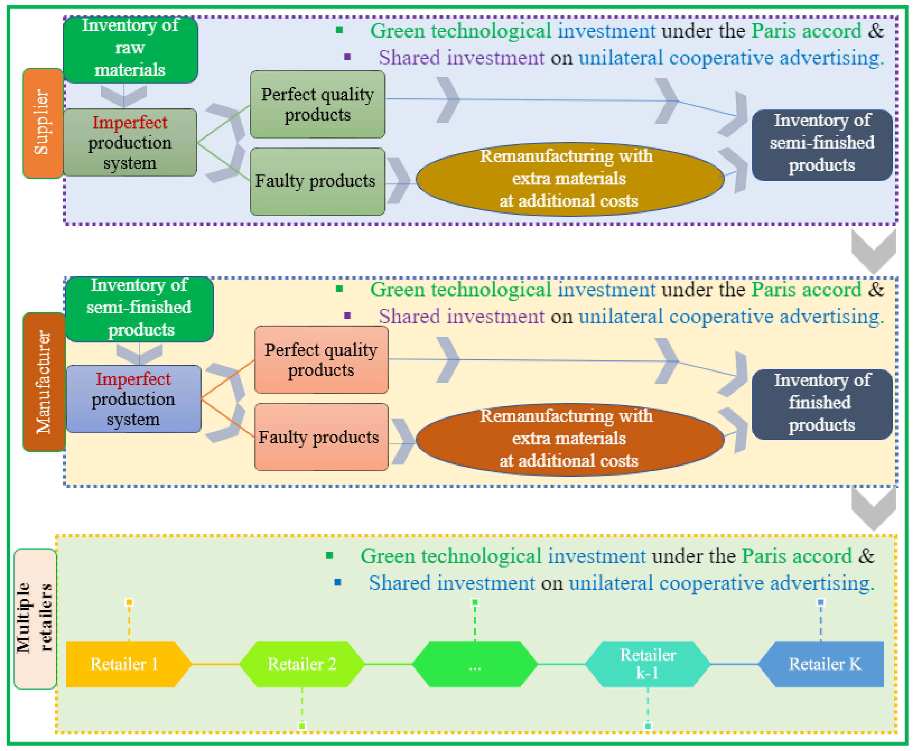
Figure 1. Graphical illustration of various aspects of the proposed SSCM model.
Logistics 07 00037 g001
Figure 2. Supplier–manufacturer inventory of the proposed SSCM model (see Sarkar et al. [10]).
Logistics 07 00037 g002
Figure 3. Manufacturer–single retailer inventory of the proposed SSCM model (see Sarkar et al. [10]).
Logistics 07 00037 g003
Figure 4. Flow chart of the algorithm to optimize fuzzy mixed-integer nonlinear programming problems.
Logistics 07 00037 g004
Figure 5. Impacts of wide-ranging demand rate over revenue and total cost.
Logistics 07 00037 g005
Figure 6. Impacts of wide-ranging demand rate of retailers over various decisions. (a) Demand rate with respect to varying cycle lengths of retailers; (b) demand rate with respect to varying aggregate advertising budget; (c) demand rate with respect to supplier’s production rate; (d) demand rate with respect to manufacturer’s production rate.
Logistics 07 00037 g006
Figure 7. Impacts of varying aggregate advertisement budget over revenue.
Logistics 07 00037 g007
Figure 8. Sensitivity analysis of several major parameters of the proposed SSCM model in Experiment I. (a) Sensitivity analysis of c ¯ d s ; (b) sensitivity analysis of c ¯ d m ; (c) sensitivity analysis of ξ ; (d) sensitivity analysis of ω s ; (e) sensitivity analysis of ω m .
Logistics 07 00037 g008
Figure 9. Sensitivity analysis of several major parameters of proposed SSCM model in Experiment II. (a) Sensitivity analysis of c ¯ d s ; (b) sensitivity analysis of c ¯ d m ; (c) sensitivity analysis of ξ ; (d) sensitivity analysis of ω s ; (e sensitivity analysis of ω m ).
Logistics 07 00037 g009
Table 1. Comparative review of recent supply chain studies.
ContributorsProduction ModelsImmediate Remanufacturing atEnvironmental AspectsOrientations
Rad et al. [24]two-stage SCvendorNA 1 crisp
Noh and Kim [3]two-echelon SCNAcontrollable CEfuzzy
Rout et al. [25]two-echelon SCmanufacturertax, cap-&-offset, cap-&-tradefuzzy inference
Shaw et al. [26]integrated inventory modelvendorcarbon taxcrisp
Kishore et al. [27]three-tier SC with faulty stockmanufacturerNAcrisp
Homayouni et al. [7]sustainable logistics modelNAcap-and-trade and carbon taxstochastic
Sarkar et al. [28]three-echelon SSCMsupplierCE related various costscrisp
Sepehri and Gholamian [29]shortages-based sustainable inventorymanufacturercarbon cap and taxcrisp
Giri and Dash [30]production inventory modelretailergreenness based demandcrisp
Adak and Mahapatra [31]two-echelon SCretailerNAcrisp
Priyan et al. [32]production inventory modelmanufacturerGTIcrisp
Present studythree-echelon SSCM modelremanufacturing at both the supplier and manufacturergreen investment of each chain partnerasymmetric TFN
1 NA: Not considered.
Table 2. Notations with descriptions of the proposed SSCM model.
• Abbreviations
S C supply chain.
S S C M sustainable supply chain management.
D M decision makers.
C E carbon emissions.
G H G greenhouse gases.
G T I green technological investment.
T F N triangular fuzzy number.
• Decision variables
G s initial GTI of supplier (USD).
G m initial GTI of manufacturer (USD).
G i r initial GTI of ith retailer (USD).
P s production rate of faulty machinery of supplier (unit/unit time).
P m production rate of faulty machinery of manufacturer (unit/unit time).
Baggregate cooperative advertisement budget of proposed model (USD).
Tcycle length of retailers (years).
• Crisp parameters
y 1 shipments of raw materials received by supplier (number).
y 2 shipment of semifinished items received by manufacturer (number).
z 1 integer multiple of manufacturer’s cycle length (number).
z 2 integer multiple of retailers’ cycle length (number).
Ffixed component of per shipment transportation cost (USD).
Vvariable component of per shipment transportation cost (USD/unit).
ξ GTI-induced CE reduction rate ( 0 ξ 1 ) (number).
θ efficiency of green technology to lower CEs ( 0 θ 1 ) (number).
δ carbon tax rate (USD/kg).
Daggregate demand rate for all retailers (unit/unit time).
α scale parameter of revenue function (number).
β shape parameter of revenue function (number).
· supplier/manufacturer (j)
Q j shipment lot size to chain partner j (number).
P j production rate at chain partner j (item per unit time).
η j system reliability parameter of chain partner j, 0 η j 1 (number).
α j variation constant related to tool and die cost (USD/unit).
c d c j fixed development cost of the imperfect production system at j (USD/unit time).
c s f i n j CEs due to holding semifinished products at chain partner j (kg/sq. ft./unit time).
b s f i n j area in inventory at partner j (sq. ft./unit).
z j quantity of CEs at chain partner j (kg).
B j quantity of CEs related to set-up at chain partner j (kg).
l j quantity of CEs related to production at chain partner j (kg/unit).
w j environmental impact of inventory (kg/unit).
B A j contribution toward cooperative advertising budget (USD).
ω j fraction of fresh raw materials during remanufacturing at j ( 0 ω j 1 ) (number).
· supplier (s)
c r a w s CEs due to holding of raw materials (kg/sq. ft./unit time).
b r a w s area in inventory for raw materials (sq. ft./unit).
·  manufacturer (m)
c f i n m CEs due to holding of raw materials (kg/sq. ft./unit time).
b f i n m area in inventory (sq. ft./unit).
· i th retailer (r)
z i r carbon allowance cost of the ith retailer (USD).
c f i n i r CEs per unit area of ith retailer (kg/sq. ft./unit time).
b f i n i r area in inventory of ith retailer (sq. ft./unit).
w r environmental impacts of inventory for any retailer (kg/unit).
d i demand rate of ith retailer (number).
a r contribution of ith retailer towards cooperative advertising ( 0 a r 1 ).
p i per unit sale price of products for the ith retailer (USD/unit).
b i r contribution of ith retailer in cooperative advertisement (USD).
B A r total contributions of all retailers on cooperative advertisement (USD).
• Parameters under fuzziness
· supplier/manufacturer (j)
c ˜ o j fuzzy material cost (USD/unit).
c ˜ d j fuzzy labor- and energy-related reworking cost of defective items (USD/unit).
a ˜ j fuzzy setup cost (USD).
o ˜ j fuzzy ordering cost (USD).
h ˜ r j holding cost of primary materials (USD/unit/unit time).
h ˜ f j holding cost of dispatchable products (USD/unit/unit time).
·ith retailer (r)
a ˜ i r fuzzy setup cost of the ith retailer (USD).
o ˜ i r fuzzy ordering cost of the ith retailer (USD).
h ˜ i r fuzzy holding cost of the ith retailer (USD/unit/unit time).
Table 3. Various crisp components of Experiment I.
Chain PartnersParametersValuesParametersValuesParametersValuesParametersValues
Supplier η s 0.4 c d c s 960.195 USD / unit time α s 0.05 β s 0.15
z s 60 kg B s 90 kg l s 40 kg c r a w s 4 kg
b r a w s 0.4  m c s f i n s 4 kg/sq.ft./unit time b s f i n s 0.4 sq.ft./unit w s 40 kg
ω s 0.1
Manufacturer η m 0.4 c d c m 960.195 USD / unit time α m 0.05 β m 0.15
z m 90 kg B m 135 kg l m 40 kg c s f i n m 4 kg/sq.ft./unit time
b s f i n m 0.4  sq.ft./unit c f i n m 4 kg/sq.ft./unit time b f i n m 0.4  sq.ft./unit w m 60 kg
ω m 0.1
ith retailer B i r 300 kg c f i n i r 4 kg/sq.ft./unit time b f i n i r 0.4  sq.ft./unit z i r 200 kg
w r 20 kg
SSCM modelFUSD  0.02 V 0.1  USD/unit ξ 0.2 θ 0.8
δ 0.22  USD/kgD 700 unit/unit time α 0 β 100
y 1 1 y 2 2 z 1 1 z 2 1
a s 0.25 a m 0.25 a r 0.5   
Table 4. Asymmetric TFN-type parameters of Experiment I.
SC PartnersParametersValues as TFNParametersValues as TFN
Supplier c ˜ 0 s ( 3 , 4 , 5 ) c ˜ d s ( 3 , 4 , 5 )
a ˜ s ( 450 , 500 , 550 ) o ˜ s ( 275 , 300 , 325 )
h ˜ r s ( 0.3 , 0.4 , 0.5 ) h ˜ f s ( 0.45 , 0.6 , 0.75 )
Manufacturer c ˜ 0 m ( 4 , 6 , 8 ) c ˜ d m ( 4 , 6 , 8 )
a ˜ m ( 180 , 200 , 220 ) o ˜ m ( 135 , 150 , 165 )
h ˜ r m ( 0.45 , 0.6 , 0.75 ) h ˜ f m ( 1.33 , 1.66 , 2 )
ith retailer a ˜ i r ( 70 , 80 , 90 ) o ˜ i r ( 6.66 , 10 , 13.33 )
h ˜ i r ( 1.33 , 1.66 , 2 )
Table 5. Optimal results of the proposed SSCM model in Experiment I.
Market UncertaintyGTI USD (Integer)Decision Variables (Continuous)Maximum Net Profit (USD)
G s * G m * G r * P s * P m * B * T *
Bullish10.0010.008.00104.1471141.14251500.000.73382,660,517.24
Stable10.0010.008.00104.8364150.41601500.000.66482,654,030.78
Bearish10.0010.008.00105.1193157.07141500.000.63232,647,636.99
Table 6. Sensitivity analysis of major parameters of the proposed SSCM model in Experiment I.
Parameters% Changes% Changes in P s * % Changes in P m * % Changes in B * % Changes in T * % Changes in NP SSCM *
c ¯ d s ( 4 ) 50−0.5666−0.05260−0.1492−0.0008
25−0.2842−0.02630−0.0749−0.0004
−250.28470.026600.07510.0004
−500.57350.053600.15160.0008
c ¯ d m ( 6 ) 50−0.0443−0.78340−0.5123−0.0557
25−0.0231−0.39420−0.2582−0.0279
−250.02290.397500.26110.0279
−500.04630.798100.52520.0557
ξ ( 0.2 ) 50−3.2817−1.487701.340.1844
25−1.616−0.733500.66870.0922
−251.56880.71380−0.6619−0.0921
−503.09441.40850−1.3201−0.1841
ω s ( 0.1 ) 50−0.0576−0.00550−0.0155−0.0001
25−0.0284−0.00270−0.00770
−250.02820.002600.00750
−500.05670.005500.01500.0001
ω m ( 0.1 ) 50−0.0062−0.07860−0.0517−0.0002
25−0.0026−0.03930−0.0259−0.0001
−250.00140.039700.02580.0001
−500.00450.079700.05220.0002
Table 7. Various crisp components of Experiment II.
Chain PartnersParametersValuesParametersValuesParametersValuesParametersValues
Supplier η s 0.4 c d c s 100 USD / unit time α s 0.05 β s 0.15
z s 150 kg B s 696 kg l s 25 kg c r a w s 0.2  kg/sq.m/unit time
b r a w s 0.02  sq.m/unit c s f i n s 0.2  kg/sq.m/unit time b s f i n s 0.02  sq.m/unit w s 464 kg
ω s 0.1
Manufacturer η m 0.4 c d c m 100 USD / unit time α m 0.05 β m 0.15
z m 150 kg B m 696 kg l m 25 kg c s f i n m 0.2  kg/sq.m/unit time
b s f i n m 0.02  sq.m/unit c f i n m 0.2  kg/sq.m/unit time b f i n m 0.02  sq.m/unit w m 464 kg
ω m 0.1
ith retailer B i r 696 kg c f i n i r 0.2  kg/sq.m/unit time b f i n i r 0.02 sq.m/unit z i r 150 kg
w r 464 kg
SSCM modelFUSD 226V 0.0041 USD / unit ξ 0.1 θ 0.2
δ 0.33  USD/kgD57 unit/unit time α 0 β 100
y 1 1 y 2 2 z 1 1 z 2 1
a s 0.25 a m 0.25 a r 0.5   
Table 8. Asymmetric TFN-type parameters of Experiment II.
SC PartnersParametersValues as TFNParametersValues as TFN
Supplier c ˜ 0 s ( 3 , 4 , 5 ) c ˜ d s ( 3 , 4 , 5 )
a ˜ s ( 300 , 400 , 500 ) o ˜ s ( 275 , 300 , 325 )
h ˜ r s ( 0.3 , 0.4 , 0.5 ) h ˜ f s ( 0.45 , 0.6 , 0.75 )
Manufacturer c ˜ 0 m ( 4 , 6 , 8 ) c ˜ d m ( 4 , 6 , 8 )
a ˜ m ( 375 , 400 , 425 ) o ˜ m ( 135 , 150 , 165 )
h ˜ r m ( 0.45 , 0.6 , 0.75 ) h ˜ f m ( 1.33 , 1.66 , 2 )
ith retailer a ˜ i r ( 90 , 100 , 110 ) o ˜ i r ( 6.66 , 10 , 13.33 )
h ˜ i r ( 1.33 , 1.66 , 2 )
Table 9. Optimal results of the proposed SSCM model in Experiment II.
Market UncertaintyGTI (USD) (Integer)Decision Variables (Continuous)Maximum Net Profit (USD)
G s * G m * G r * P s * P m * B * T *
Bullish34.0034.0034.0016.338630.62881700.004.9207208,679.57
Stable33.0033.0033.0017.053532.29261700.004.0330207,589.38
Bearish33.0033.0032.0017.211232.77571700.003.6296206,554.74
Table 10. Sensitivity analysis of major parameters of the proposed SSCM model in Experiment II.
Parameters% Changes% Changes in P s * % Changes in P m * % Changes in B * % Changes in T * % Changes in NP SSCM *
c ¯ d s ( 4 ) 5000000
259.21610.029801.89280.0089
−25−7.1638−0.19010−1.5313−0.008
−5000000
c ¯ d m ( 6 ) 50−0.4705−6.81160−4.0892−0.0938
25−0.2364−3.63030−2.2018−0.0473
−250.23134.225902.63500.0483
−500.43869.284805.90430.0980
ξ ( 0.1 ) 50−0.0223−0.0280−0.1970.6523
25−0.0113−0.01380−0.09550.3261
−250.00960.01300.0862−0.326
−500.01820.023600.1556−0.6519
ω s ( 0.1 ) 50−0.7949−0.01980−0.1669−0.0008
25−0.4001−0.00990−0.0839−0.0004
−250.40450.010100.08480.0004
−500.81520.020000.17050.0008
ω m ( 0.1 ) 50−0.0470−0.76810−0.4704−0.0023
25−0.0237−0.38680−0.2372−0.0012
−250.02350.392800.24150.0012
−500.04700.791900.48750.0024
Table 11. Comparison of current study with some well-established articles.
ContributorsFormulationMethodologyResults and Insights
Model typeRemanufacturing policyVariables and AnalysisDefuzzification
Sarkar et al. [13]EPQ modeltime-varying malfunctioning rate of manufacturerclassical optimizationNA
  • with quadratic demand rate and inflation, varying reliability is beneficial.
Soni et al. [45]EPQ modelproduct quality improvement by manufactureroptimization algorithmmodified graded mean integration representation
  • cost components affected by fuzziness impact overall cost;
  • positive decisions are more advantageous than negative ones.
Sarkar et al. [10]three-echelon SCNAsequential quadratic programmingsigned distance method
  • supplier’s and manufacturer’s holding costs have impacts on profitability;
  • an evenly distributed advertising expenditure increases demand and profitability;
  • a cut in production rate improves net profit.
Mishra et al. [6]inventory modelNAclassical optimizationNA
  • profits are boosted by higher sale prices and efficient technology;
  • items that deteriorate slowly maximize the retailer’s profit.
Rout et al. [25]sustainable SCreworking on imperfect production at manufacturernondominated shortingMamdani fuzzy inference
  • instead of scrapping defective products, remanufacture them.
Present studyeconomic and ecofriendly three-echelon SC modelremanufacturing with labor and fresh materials by both supplier and manufacturerclassical optimization methoddegree-of-optimism-based total λ -integral method
  • slower production by supplier and manufacturer, plus an extended cycle, yielding more profit in a growing market;
  • reduced quantity of faulty products, plus GTI-induced reduction in CEs enhances the profitability.
Disclaimer/Publisher’s Note: The statements, opinions and data contained in all publications are solely those of the individual author(s) and contributor(s) and not of MDPI and/or the editor(s). MDPI and/or the editor(s) disclaim responsibility for any injury to people or property resulting from any ideas, methods, instructions or products referred to in the content.