
International Transportation Mode Selection through Total Logistics Cost-Based Intelligent Approach


Abstract
:1. Introduction
2. Literature Review
3. Methodology
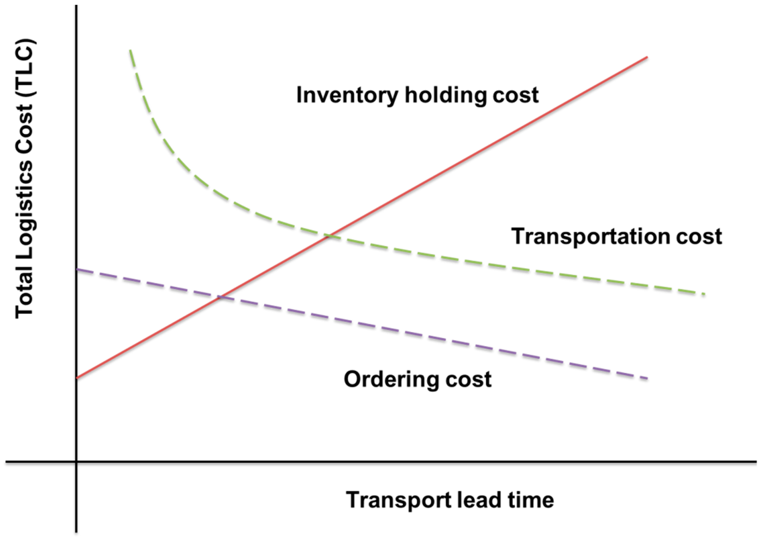
3.1. Components of Total Logistics Cost
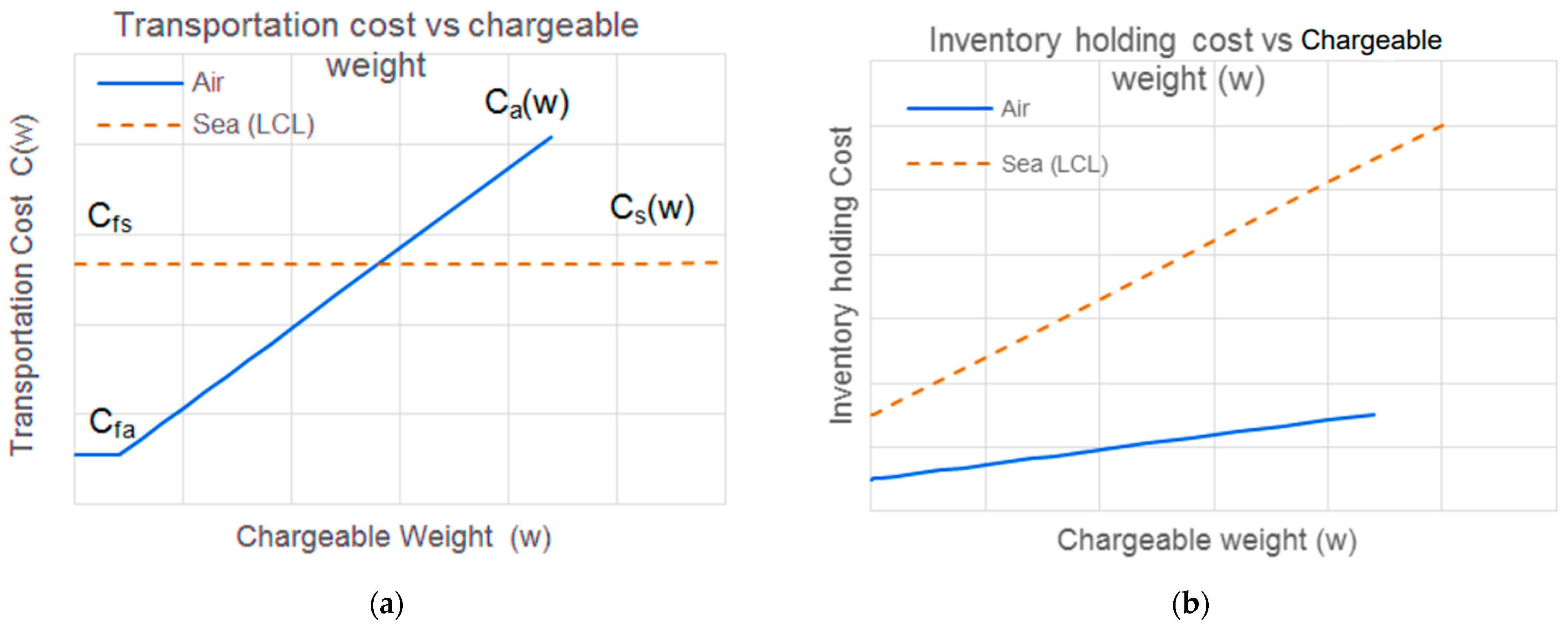
3.1.1. Transportation Cost
3.1.2. Inventory Holding Cost
3.1.3. Ordering Cost
4. Case Studies, Results, and Discussion
4.1. Determining Freight Mode for Regularly Replenished Products
4.1.1. Case I: Regular Replenishment of the Same Product
- Origin country: Germany, Destination country: India
- Origin airport: Frankfurt, Destination airport: Mumbai
- Origin seaport: Bremerhaven, Destination seaport: Mumbai
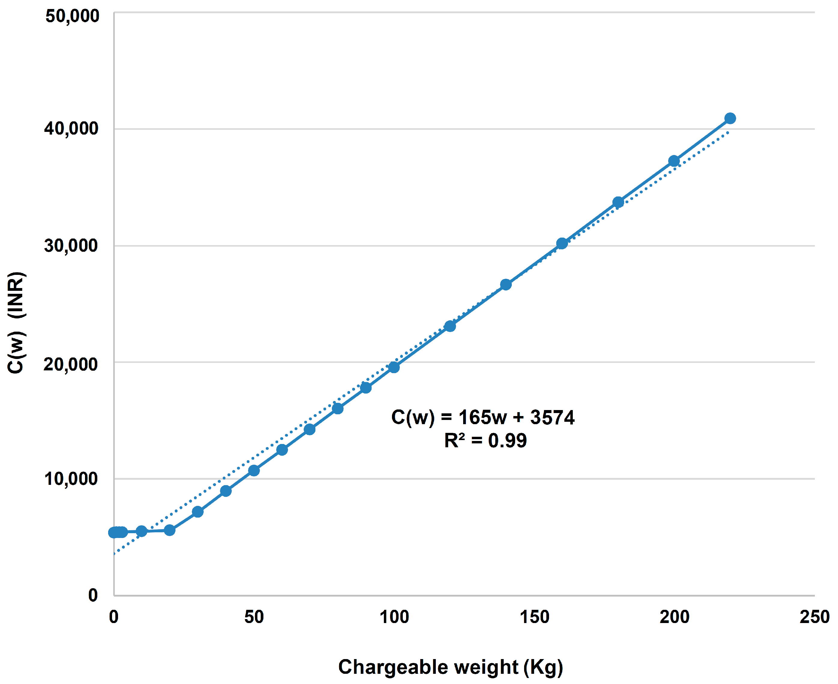
Transportation Cost Considering Air Mode
Transportation Cost (Sea Mode (LCL))
Optimization for Sea Shipping
Optimization for Air Shipping
4.1.2. Case II: Regular Replenishment of Multiple Types of Products
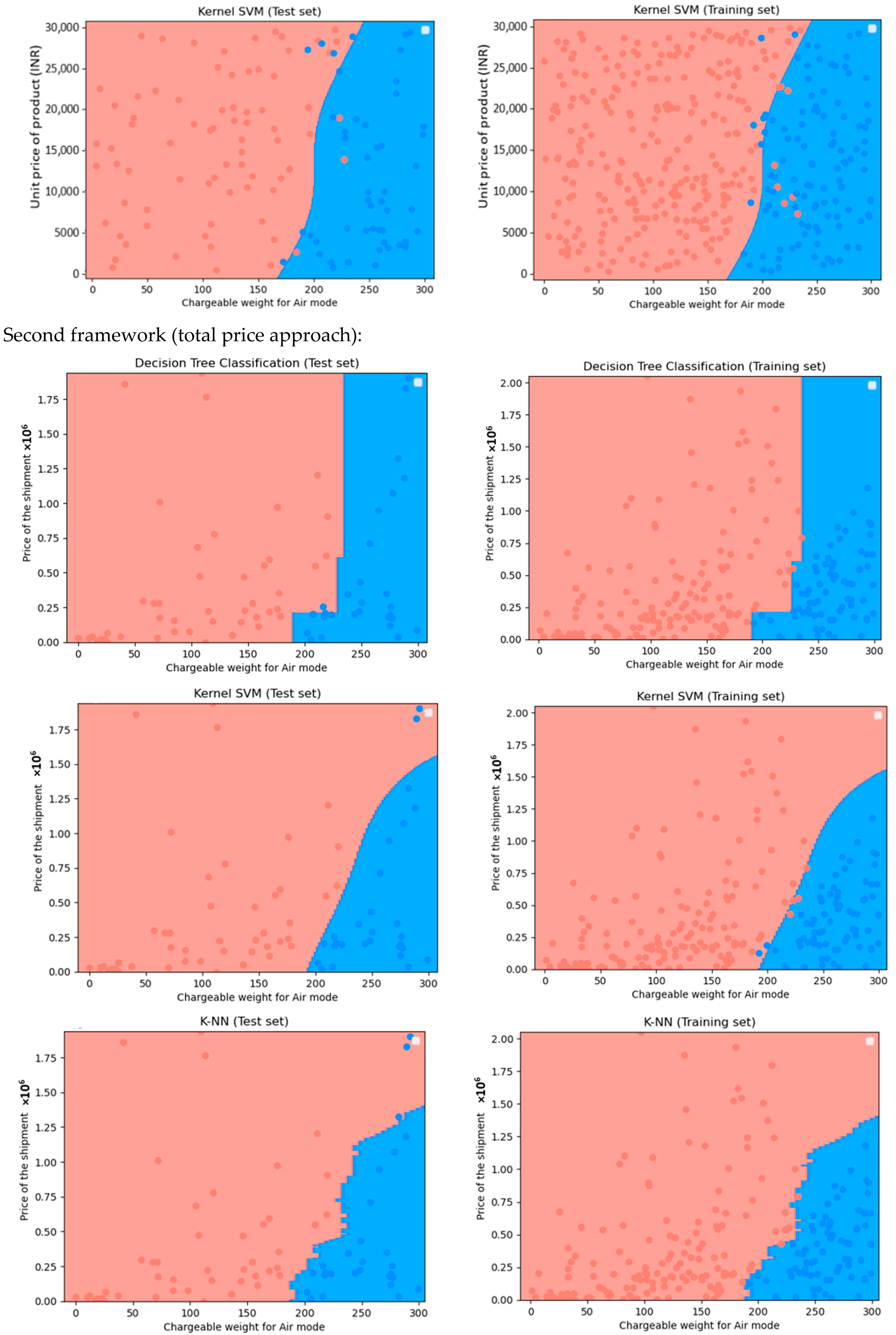
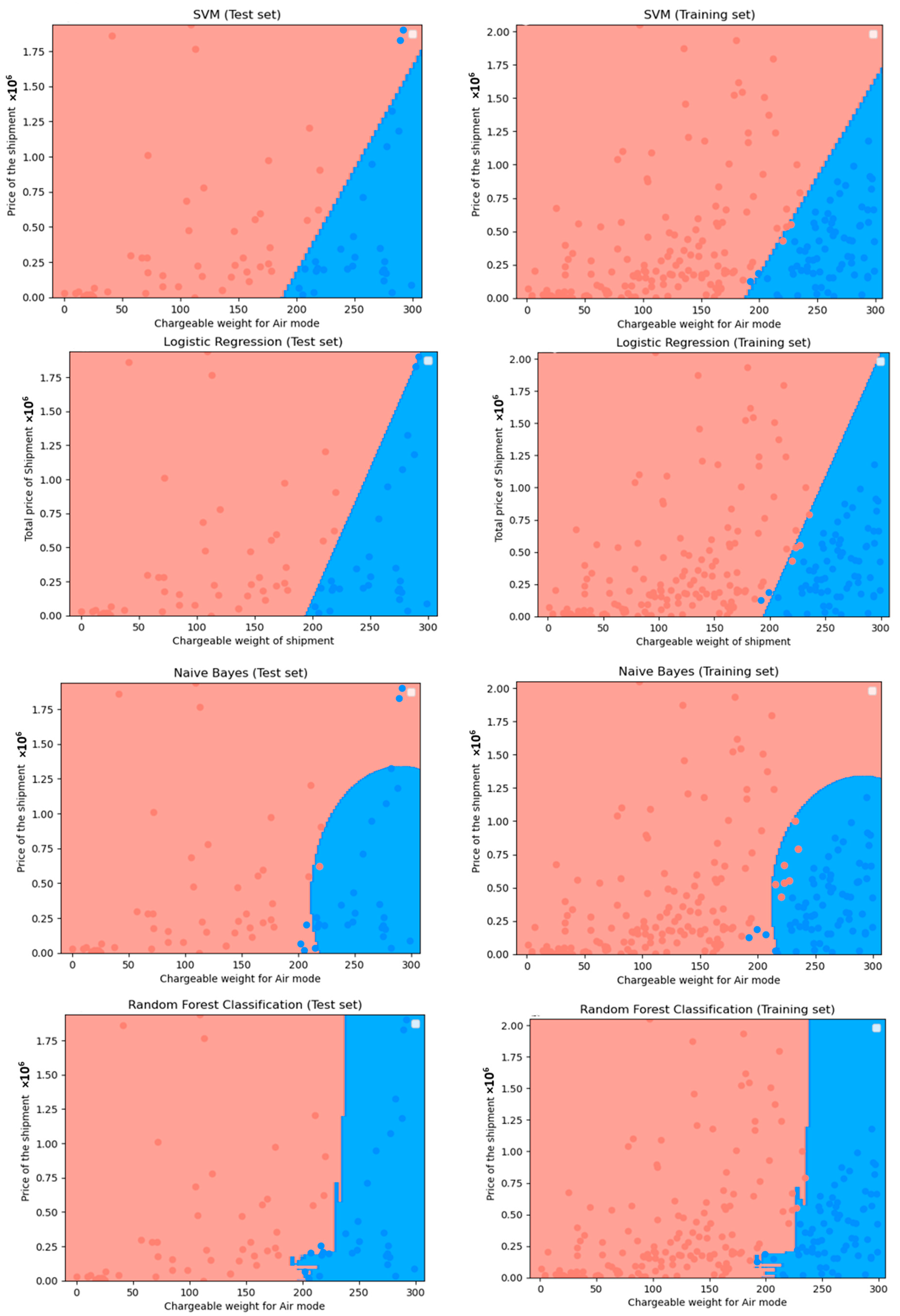
4.2. Determining the Freight Mode of Any Shipment
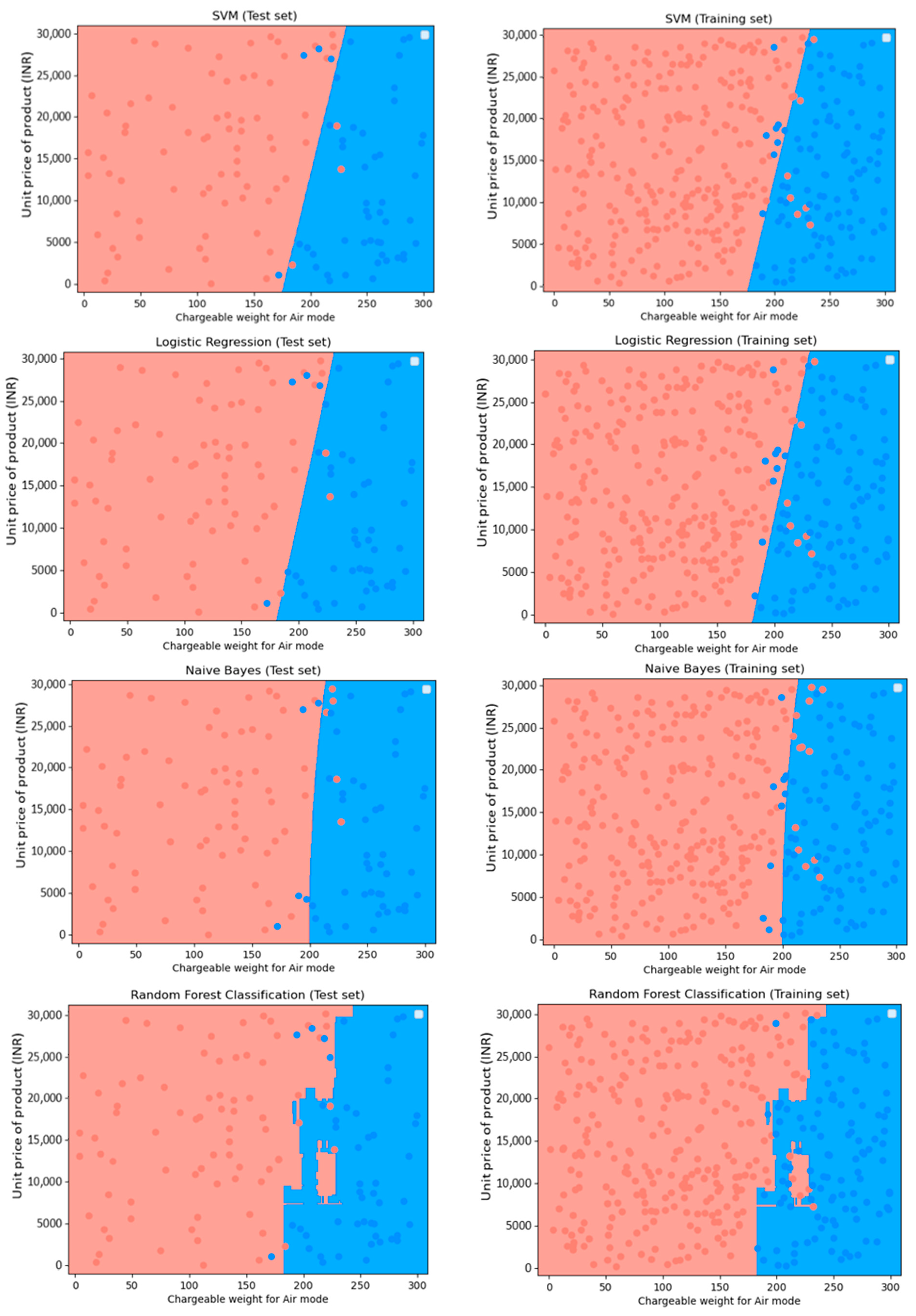
4.2.1. Machine Learning-Based Classification
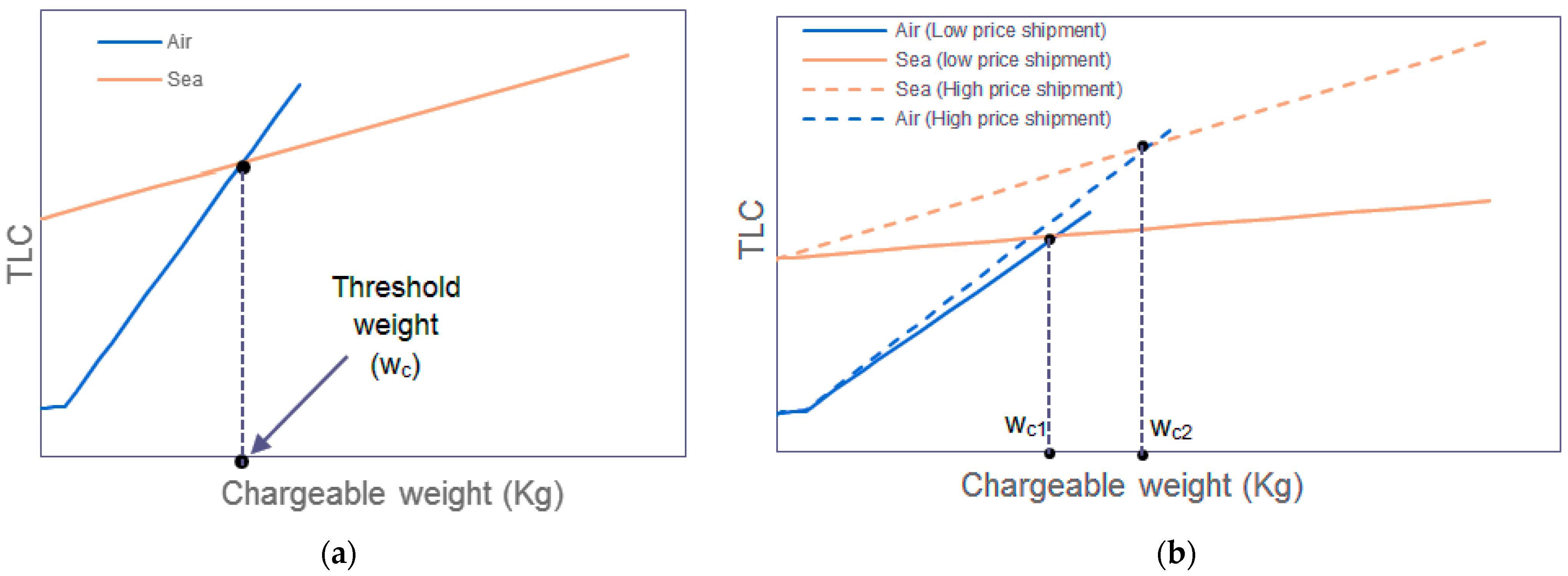
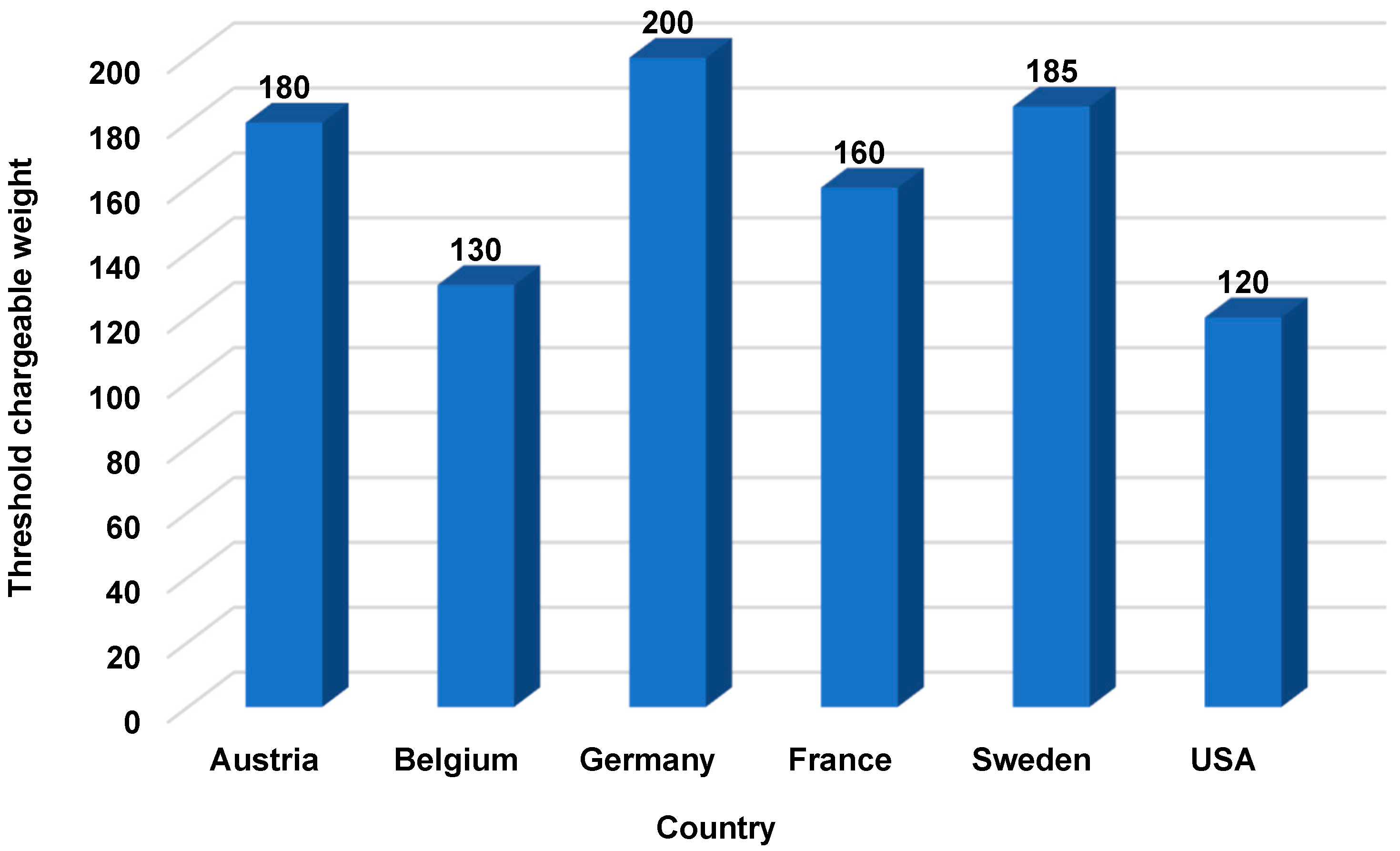
4.2.2. Establishing Threshold for Chargeable Weight
4.3. Impact of Inventory Holding Rates on Transportation Mode Selection
5. Conclusions, Limitations, and Future Research Avenues
Author Contributions
Funding
Institutional Review Board Statement
Informed Consent Statement
Data Availability Statement
Conflicts of Interest
Appendix A

References
- Lovell, A.; Saw, R.; Stimson, J. Product value-density: Managing diversity through supply chain segmentation. Int. J. Logist. Manag. 2005, 16, 142–158. [Google Scholar] [CrossRef]
- Tate, W.L.; Bals, L. Outsourcing/offshoring insights: Going beyond reshoring to rightshoring. Int. J. Phys. Distrib. Logist. Manag. 2017, 47, 106–113. [Google Scholar] [CrossRef]
- Ceniga, P.; Sukalova, V. Future of Logistics Management in the Process of Globalization. Procedia Econ. Financ. 2015, 16, 160–166. [Google Scholar] [CrossRef]
- Saldanha, J.P.; Tyworth, J.E.; Swan, P.F.; Russell, D.M. Cutting logistics cost with ocean carrier selection. J. Bus. Logist. 2009, 30, 175–195. [Google Scholar] [CrossRef]
- Prajapati, D.; Kumar, M.M.; Pratap, S.; Chelladurai, H.; Zuhair, M. Sustainable Logistics Network Design for Delivery Operations with Time Horizons in B2B E-Commerce Platform. Logistics 2021, 5, 61. [Google Scholar] [CrossRef]
- Meixell, M.J.; Norbis, M. A Review of the Transportation Mode Choice And Carrier Selection Literature. Int. J. Logist. Manag. 2008, 19, 183–211. [Google Scholar] [CrossRef]
- Song, D. A Literature Review, Container Shipping Supply Chain: Planning Problems and Research Opportunities. Logistics 2021, 5, 41. [Google Scholar] [CrossRef]
- Rodrigue, J.P. Chapter 5: International trade and freight distribution. In The Geography of Transport Systems, 3rd ed.; Routledge Publisher: London, UK, 2013; pp. 158–183. [Google Scholar]
- Achahchah, M. Transportation, Lean Transportation Management: Using Logistics as a Strategic Differentiator, 1st ed.; Taylor and Francis Group; Productivity Press: New York, NY, USA, 2018; Chapter 2; pp. 44–111. [Google Scholar] [CrossRef]
- Feng, B.; Li, Y.; Shen, Z.-J.M. Air cargo operations: Literature review and comparison with practices. Transp. Res. Part C Emerg. Technol. 2015, 56, 263–280. [Google Scholar] [CrossRef]
- Jung, H.; Kim, J.; Shin, K. Importance Analysis of Decision Making Factors for Selecting International Freight Transportation Mode. Asian J. Shipp. Logist. 2019, 35, 55–62. [Google Scholar] [CrossRef]
- Fallah, S. 11—Customer Service. In Logistics Operations Management; Farahani, R.Z., Razapour, S., Kardar, L., Eds.; Elsevier: Amsterdam, The Netherlands, 2011; pp. 199–218. [Google Scholar] [CrossRef]
- Bang, K.T.; Jang, H.H. An empirical study on the transport mode selection factors of Korean exporters -based on the control factor of manufacturing and logistics industry. J. Shipp. Logist. 2011, 69, 245–263. [Google Scholar] [CrossRef]
- Neumann, T. Comparative Analysis of Long-Distance Transportation with the Example of Sea and Rail Transport. Energies 2021, 14, 1689. [Google Scholar] [CrossRef]
- Bartulović, D.; Abramović, B.; Brnjac, N.; Steiner, S. Role of air freight transport in intermodal supply chains. Transp. Res. Procedia 2022, 64, 119–127. [Google Scholar] [CrossRef]
- Černá, L.; Zitrický, V.; Daniš, J. The Methodology of Selecting the Transport Mode for Companies on the Slovak Transport Market. Open Eng. 2017, 7, 6–13. [Google Scholar] [CrossRef]
- Patil, R.; Rahegaonkar, A.; Patange, A.; Nalavade, S. Designing an optimized schedule of transit electric bus charging: A municipal level case study. Mater. Today Proc. 2022, 56, 2653–2658. [Google Scholar] [CrossRef]
- Galindo-Pacheco, G.M.; Paternina-Arboleda, C.D.; Barbosa-Correa, R.A.; Llinás-Solano, H. Non-linear programming model for cost minimisation in a supply chain, including non-quality and inspection costs. Int. J. Oper. Res. 2012, 14, 301–323. [Google Scholar] [CrossRef]
- Tirkolaee, E.B.; Sadeghi, S.; Mooseloo, F.M.; Vandchali, H.R.; Aeini, S. Application of Machine Learning in Supply Chain Management: A Comprehensive Overview of the Main Areas. Math. Probl. Eng. Hindawi 2021, 2021, 1476043. [Google Scholar] [CrossRef]
- Beresford, A.K.C.; Banomyong, R.; Pettit, S. A Critical Review of a Holistic Model Used for Assessing Multimodal Transport Systems. Logistics 2021, 5, 11. [Google Scholar] [CrossRef]
- Vasilev, J.; Milkova, T. Optimisation Models for Inventory Management with Limited Number of Stock Items. Logistics 2022, 6, 54. [Google Scholar] [CrossRef]
- Tsolaki, K.; Vafeiadis, T.; Nizamis, A.; Ioannidis, D.; Tzovaras, D. Utilizing machine learning on freight transportation and logistics applications: A review. ICT Express 2022, 9, 284–295. [Google Scholar] [CrossRef]
- Singh, A.; Wiktorsson, M.; Hauge, J.B. Trends in Machine Learning To Solve Problems In Logistics. Procedia CIRP 2021, 103, 67–72. [Google Scholar] [CrossRef]
- Chang, C.H.; Thai, V.V. Shippers’ choice behaviour in choosing transport mode: The case of South East Asia (SEA) region. Asian J. Shipp. Logist. 2017, 33, 199–210. [Google Scholar] [CrossRef]
- Ballou, R.H.; Srivastava, S.K. Business Logistics/Supply Chain Management: Planning, Organizing, and Controlling the Supply Chain; Pearson Education India: Chennai, India, 2007. [Google Scholar]
- Zeng, A. Developing a framework for evaluating the logistics costs in global sourcing processes: An implementation and insights. Int. J. Phys. Distrib. Logist. Manag. 2003, 33, 785–803. [Google Scholar] [CrossRef]
- Santoso, S.; Nurhidayat, R.; Mahmud, G.; Arijuddin, A.M. Measuring the Total Logistics Costs at the Macro Level: A Study of Indonesia. Logistics 2021, 5, 68. [Google Scholar] [CrossRef]
- Davis, P. Incoterms® 2020 and the missed opportunities for the next version. Int. J. Logist. Res. Appl. 2021, 30, 1263–1286. [Google Scholar] [CrossRef]
- Vogt, J.; Davis, J. The State of Incoterm® Research. Transp. J. 2020, 59, 304–324. [Google Scholar] [CrossRef]
- Azzi, A. Inventory holding costs measurement: A multi-case study. Int. J. Logist. Manag. 2014, 25, 109–132. [Google Scholar] [CrossRef]
- Tony Arnold, J.R. Chapter 9—Inventory Fundamentals, Introduction to Materials Management; Pearson Prentice-Hall: Hoboken, NJ, USA, 2004; pp. 254–280. [Google Scholar]
- Deniz, B.; Karaesmen, I.; Scheller-Wolf, A. A comparison of inventory policies for perishable goods. Oper. Res. Lett. 2020, 48, 805–810. [Google Scholar] [CrossRef]
- Önal, M. The two-level economic lot sizing problem with perishable items. Oper. Res. Lett. 2016, 44, 403–408. [Google Scholar] [CrossRef]
- Biswas, S.; Bandyopadhyay, G.; Mukhopadhyaya, J.N. A multi-criteria based analytic framework for exploring the impact of Covid-19 on firm performance in emerging market. Decis. Anal. J. 2022, 5, 100143. [Google Scholar] [CrossRef]
- Xidonas, P.; Steuer, R. A multicriteria evaluation methodology for assessing the impact of COVID-19 in EU countries. Decis. Anal. J. 2022, 4, 100123. [Google Scholar] [CrossRef]
- Pujawan, I.N.; Bah, A.U. Supply chains under COVID-19 disruptions: Literature review and research agenda. Supply Chain Forum 2021, 23, 81–95. [Google Scholar] [CrossRef]
- Hossain, M.R.; Akhter, F.; Sultana, M.M. SMEs in Covid-19 Crisis and Combating Strategies: A Systematic Literature Review (SLR) and A Case from Emerging Economy. Oper. Res. Perspect. 2022, 9, 2214–7160. [Google Scholar] [CrossRef]


| Parameter | Value |
|---|---|
| Value of the product (V) | 7000 INR * |
| Unit weight of the product (U) | 3.5 Kgs |
| Unit volume of the packaged product (L) | 0.018 m3 |
| Average monthly demand for the product | 230 units |
| Average demand per day (d) | ~8 units |
| The time horizon for optimization (t) | 1 month |
| Inventory holding rate (I) | 25% per annum |
| Transit lead time for sea mode (Ts) | 55 days |
| Transit lead time for air mode (Ta) | 6 days |
| Average lead time variation ΔT for sea | 14 days |
| Average lead time variation ΔT for air | 2 days |
| Ordering cost (z) | 1000 INR * |
| Product Features | ||||||||
|---|---|---|---|---|---|---|---|---|
| Product | U (Kg) | L (m3) | V (INR) | Monthly Avg. Sales | W (Kg) for Air | |||
| Product 1 | 3.50 | 0.0180 | 7000 | 90 | 158 | |||
| Product 2 | 1.00 | 0.0120 | 3000 | 14 | 14 | |||
| Product 3 | 2.00 | 0.0120 | 4500 | 8 | 8 | |||
| The Optimal Solution for Air Freight | The Optimal Solution for Sea Freight | |||||||
| n | q | Minimized TLC after Optimization | n | q | Minimized TLC after Optimization | |||
| Product 1 | 2 | 45 | 77,062 | 1 | 90 | 86,568 | ||
| Product 2 | 2 | 7 | 1 | 14 | ||||
| Product 3 | 2 | 4 | 1 | 8 | ||||
| Chargeable Weight for Air Mode (Kg) | Unit Price of a Product in (INR) | Expected Mode of Shipment |
|---|---|---|
| 22 | 3072 | Air |
| 242 | 5690 | Sea |
| 119 | 27,088 | Air |
| 190 | 4828 | Sea |
| 84 | 11,948 | Air |
| Classifier | Type | Accuracy |
|---|---|---|
| Logistic regression | Linear | 95.2% |
| K-NN | Non-linear | 92.0% |
| Linear SVM | Linear | 94.4% |
| Kernel SVM | Non-linear | 92.8% |
| Naïve Bayes | Non-linear | 92.0% |
| Decision tree | Non-linear | 93.6% |
| Random forest | Non-linear | 93.6% |
| Predicted | |||
|---|---|---|---|
| Air | Sea | ||
| Actual | Air | 74 | 2 |
| Sea | 4 | 45 | |
| Chargeable Weight for Air Mode (Kg) | Total Price of a Shipment (INR) | Expected Mode of Shipment |
|---|---|---|
| 32 | 46,638 | Air |
| 119 | 605,968 | Air |
| 85 | 76,704 | Air |
| 274 | 182,434 | Sea |
| 164 | 552,017 | Air |
| Classifier | Type | Accuracy |
|---|---|---|
| Logistic regression | Linear | 98.6% |
| K-NN | Non-linear | 96.0% |
| Linear SVM | Linear | 97.3% |
| Kernel SVM | Non-linear | 97.3% |
| Naïve Bayes | Non-linear | 90.6% |
| Decision tree | Non-linear | 98.0% |
| Random forest | Non-linear | 94.6% |
| Predicted | |||
|---|---|---|---|
| Air | Sea | ||
| Actual | Air | 47 | 0 |
| Sea | 1 | 27 | |
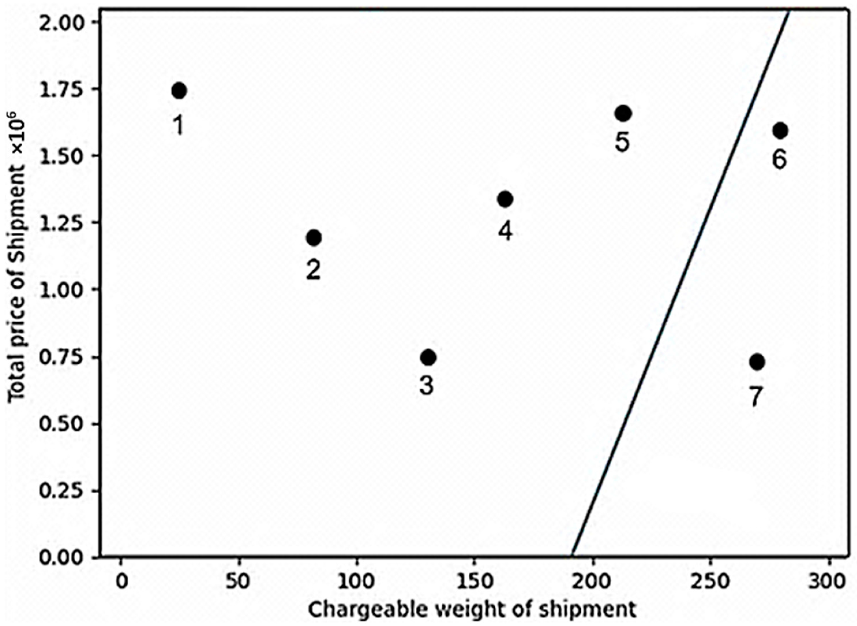
| Shipment No. | Total Price of the Shipment | Chargeable Weight for Air | Prediction | Probabilities | |
|---|---|---|---|---|---|
| Air | Sea | ||||
| 1 | 1.75 × 10⁶ | 25 | Air | 1 | 0 |
| 2 | 1.21 × 10⁶ | 80 | Air | ~1 | 0 |
| 3 | 0.75 × 10⁶ | 130 | Air | ~1 | 0 |
| 4 | 1.37 × 10⁶ | 162 | Air | 0.99 | 0.01 |
| 5 | 1.70 × 10⁶ | 212 | Air | 0.96 | 0.04 |
| 6 | 1.57 × 10⁶ | 280 | Sea | 0.33 | 0.67 |
| 7 | 0.73 × 10⁶ | 268 | Sea | 0.10 | 0.90 |
Disclaimer/Publisher’s Note: The statements, opinions and data contained in all publications are solely those of the individual author(s) and contributor(s) and not of MDPI and/or the editor(s). MDPI and/or the editor(s) disclaim responsibility for any injury to people or property resulting from any ideas, methods, instructions or products referred to in the content. |
© 2023 by the authors. Licensee MDPI, Basel, Switzerland. This article is an open access article distributed under the terms and conditions of the Creative Commons Attribution (CC BY) license (https://creativecommons.org/licenses/by/4.0/).
Share and Cite
Patil, R.A.; Patange, A.D.; Pardeshi, S.S. International Transportation Mode Selection through Total Logistics Cost-Based Intelligent Approach. Logistics 2023, 7, 60. https://doi.org/10.3390/logistics7030060
Patil RA, Patange AD, Pardeshi SS. International Transportation Mode Selection through Total Logistics Cost-Based Intelligent Approach. Logistics. 2023; 7(3):60. https://doi.org/10.3390/logistics7030060
Chicago/Turabian StylePatil, Rushikesh A., Abhishek D. Patange, and Sujit S. Pardeshi. 2023. "International Transportation Mode Selection through Total Logistics Cost-Based Intelligent Approach" Logistics 7, no. 3: 60. https://doi.org/10.3390/logistics7030060
APA StylePatil, R. A., Patange, A. D., & Pardeshi, S. S. (2023). International Transportation Mode Selection through Total Logistics Cost-Based Intelligent Approach. Logistics, 7(3), 60. https://doi.org/10.3390/logistics7030060