Figure 3,
Figure 4,
Figure 5 and
Figure 6 compare this work with the existing literature presented in
Figure 1 and
Figure 2,
Section 1.1.
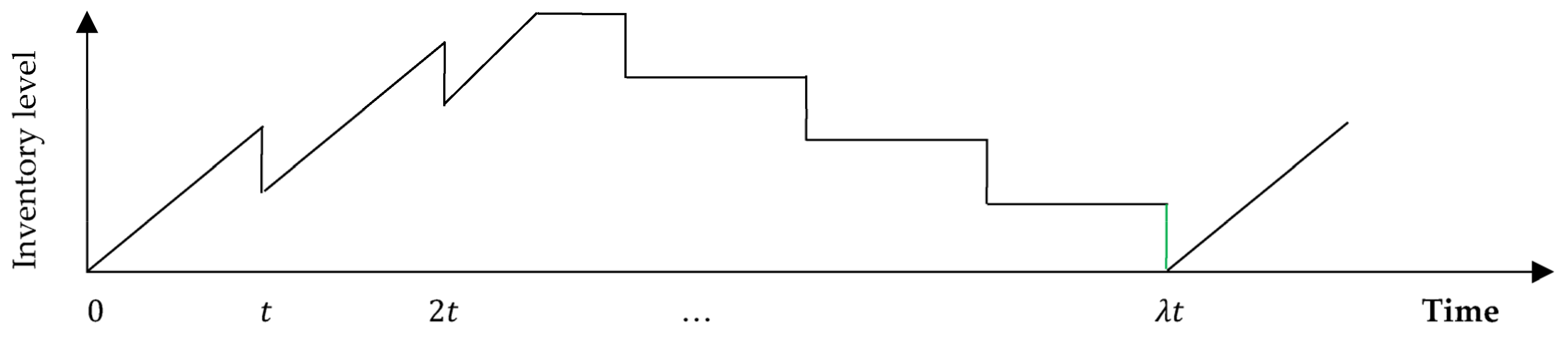
Figure 3 and
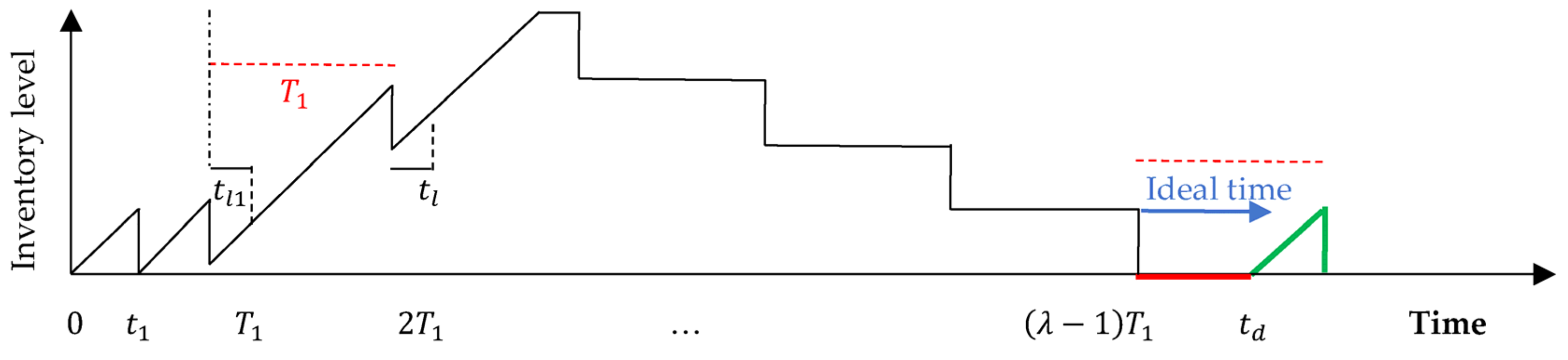
Figure 4 represent, respectively, the inventory status of the proposed joint model for the vendor and the buyer for the first cycle, whereas
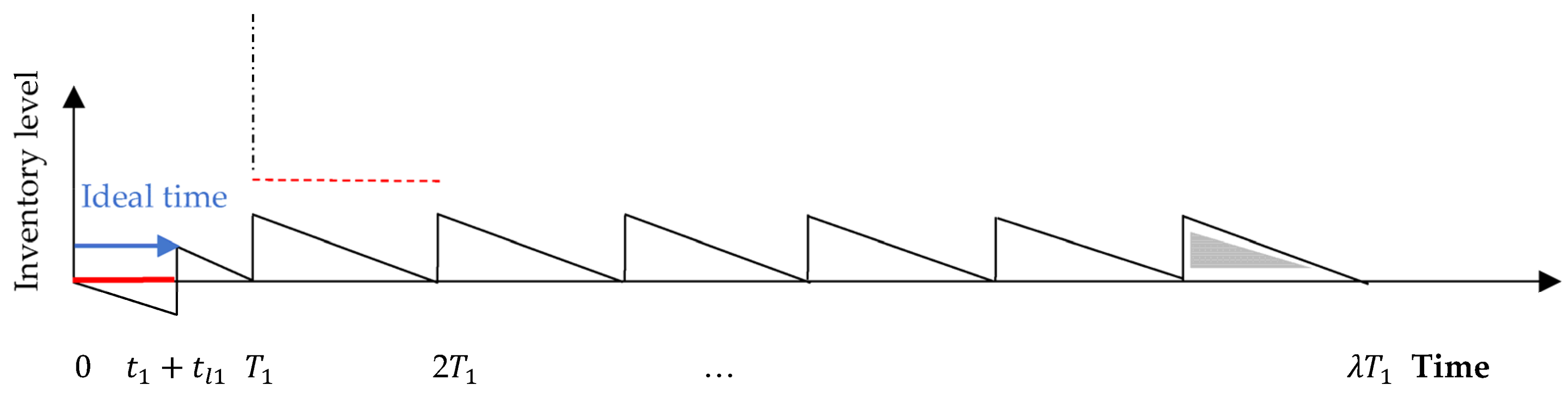
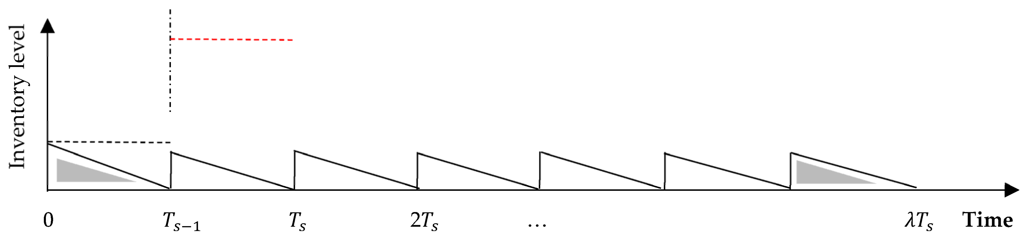
Figure 5 and
Figure 6 represent, respectively, the inventory status of the proposed joint model for the vendor and the buyer for subsequent cycles. In the proposed joint model, production commences at the beginning of the first cycle at a rate
until time
, where
units have been produced (
Figure 3). At this time, i.e.,
, this amount is delivered to the buyer to fully satisfy backordered demand that has been accumulated during production period
and transportation period
, i.e., demand that covers the time
and to satisfy demand until time
(
Figure 4).
Note that during the first cycle
,
Figure 3 and
Figure 4 indicate that the vendor and the buyer incur a holding cost that applies for
lots, since by time
, the vendor must then have delivered two lots. That said, the first lot is delivered at time
, which arrives at the buyer at time
, whereas the second lot arrives just before the first lot is consumed, i.e., at time
. It is worth noting here that such modeling tractability would clear any discrepancy resulting from
Figure 1 and
Figure 2. More specifically, in
Figure 4, the initial inventory level at the beginning of the first cycle is zero, whereas in
Figure 6, the inventory level at the beginning of a cycle represents the quantity of the last lot produced in the previous cycle. Similarly, in
Figure 3, the vendor delivers the first lot at time
. In
Figure 3 and
Figure 5, the last lot produced in the first (subsequent) cycle satisfies the demand for the last period (time
(
) in
Figure 4 and
Figure 6). However, and for illustrative purposes only, it constitutes the first lot (for time
in
Figure 6) in the buyer warehouse in the subsequent cycles, though its associated costs are included in the previous cycle. For holding cost reduction, the re-start-up production time is displaced until time
to allow consuming the last lot that has been replenished to the buyer in the previous cycle. In this case,
, which satisfies the demand for the buyer during the period
.
From a mathematical point of view, the last lot produced in the previous cycle constitutes the last lot replenished to the buyer in that same previous cycle. This implies that the costs associated with such a lot should be included in the total cost function of the previous cycle. Moreover, the fact that the inventory fluctuation in the first cycle differs from that in the second cycle would suggest a distinct optimal lot size for the second cycle. From a mathematical and practical point of view, it is often the case that the decision-maker may face a situation that requires input parameters to be adjusted to be compatible with a new policy. Unlike previous works, the lot size produced in a cycle may differ from previous lots. This entails a production policy that generates equal or unequal quantities that are associated with a fixed multiplier for each distinct cycle, and consequently, the production process is dynamic in all cycles, including the first-time interval. As can be seen,
Figure 3,
Figure 4,
Figure 5 and
Figure 6 guarantee that the quantity produced for each lot together with its associated multiplier are independent for each cycle, i.e., they are independent from previous cycles. Moreover,
Figure 3,
Figure 4,
Figure 5 and
Figure 6 indicate that both the vendor and the buyer incur a holding cost that applies to
lots. Note that in
Figure 6, the production, holding, and transportation costs of the first lot (the last lot that has been produced in the previous cycle) are considered for that same previous cycle but have been ignored in cycle
. Similarly, in
Figure 6, the ordering and holding costs of the first lot that has been produced in the previous cycle have been ignored in cycle
; however, are considered for that same previous cycle.
Figure 7 depicts the CO
2 emissions associated with the activities in the vendor and buyer warehouses. The direct emission level related to the buyer occurs due to keeping items in storage, whereas the direct emission level related to the vendor is influenced by producing the required quantity as well as keeping such quantity in storage. The direct emission level related to the vendor also includes the weight of the items delivered to the buyer. The indirect emission level related to the vendor comprises the number of shipments, fuel consumption, the distance between the vendor and the freight, and the distance between the vendor and the buyer.
3.3.1. Total Cost Function for the First Cycle under a Centralized Scenario
The inventory level of the first lot depicted in
Figure 3 for the vendor is at its maximum, i.e.,
at time
, which satisfies demand and shortages.
At time , a lot of size units should be replenished to the buyer in a duration of transportation time , to satisfy demand and shortages.
This quantity is given by:
At time
,
units have been backordered and consequently, the maximum inventory level is
units (
Figure 4). Therefore, the time required to consume the first lot is given by:
As can be seen,
Figure 4 reflects the fact that the buyer’s initial inventory level at the beginning of the first cycle is zero, whereas
Figure 3 reflects the fact that the last lot produced in the first cycle constitutes the last lot replenished to the buyer in the first cycle as well. Therefore, we have
Remark 1. The vendor may use a combination of LTL and TL services to arrange the shipment of the order quantity.
Let denotes a quantity for which the cost of transportation by either service is identical and refers to the proportion of vehicle capacity that needs to be assigned for vehicle if TL service is considered. Therefore, we distinguish two cases:
In case one, the system uses a combination of LTL and TL services to arrange the shipment of the order quantity, i.e., vehicles of TL service, and transport the rest of the items using LTL service. In this case, .
In case two, the system uses vehicles of the TL service to arrange the shipment of the order quantity. In this case, .
Let denote a pure transportation policy of implementing the TL service, and refers to a mixed policy for which a combination of LTL and TL services is utilized.
From
Figure 3 and
Figure 4, and Equations (1) and (2), the holding costs per unit time (see
Appendix A) for the buyer and the vendor are, respectively, given by:
Remark 2. In addition to the holding cost, both the buyer and the vendor experience the cost associated with emissions
being released while keeping items in storage, which depends on both inventory levels, i.e., Equations (3) and (4) [
31,
40,
56,
57].
By Remark 1, the fixed transportation costs per unit time for the vendor is given by:
The vendor incurs costs associated with emissions from production due to producing
units and delivering this quantity to the buyer. Therefore, the variable transportation and emissions costs per unit of time for the vendor are as follows:
The total amount of emissions generated by the system is given by:
From which, the cap-and-trade regulations are given by:
Equation (8) implies that the system earns revenue from selling excess quota if and only if .
Considering the above along with set-up, ordering, and investment cost components, the total cost functions per unit time for the buyer and the vendor are, respectively, given by:
The term implies that the higher the investment cost offered by the vendor, the closer the items become greener, and, consequently, the system reaps the benefit of such investment by reducing the cost incurred for emissions generated from production.
Now for simplicity, let , , and .
Therefore, the total joint cost function per unit time for the buyer and the vendor is given by:
The objective is to find integer values of that minimize where is given by Equation (11).
Hence, the objective is to solve the following optimization problem:
Thus, from Theorem 1 (see
Appendix B), a two-step solution approach is provided below:
Step 1:
Find with an integer value that minimizes either or given by Equation (A12) or Equation (A13). Alternatively, start with and compute the first three terms of Equation (A12) or Equation (A13) and continue the search by adding 1 each time until Equation (A12) or Equation (A13) attains its minimum.
Step 2:
Using Equation (A11), find , if , then set in Equation (11). Else, i.e., , then set in Equation (11) and compute from Equation (7). Note that constitutes two numbers, i.e., the integer value of plus the value of the fraction .
In a decentralized, uncoordinated scenario, the buyer orders according to the EOQ formula, and the vendor optimizes the production-inventory policy such that a LFL is replenished for the buyer. In a decentralized, coordinated scenario, the buyer orders according to the EOQ formula, and the vendor in turn must adjust, using , the production-inventory policy, to replenish a multiple of this quantity. In this case, resulted from the EOQ formula of the buyer is used to find , if , then set in Equation (11). Else, i.e., , then set in Equation (11).
3.3.2. Total Cost Function for Subsequent Cycles under a Centralized Scenario
The inventory level of the first lot depicted in
Figure 5 for the vendor is at its maximum, i.e.,
at time
. Note that the re-start-up production time is displaced until time
to allow consuming the last lot that has been replenished to the buyer in the previous cycle. In this case,
, which satisfies demand for the buyer during the period
.
At time
, a lot of size
units should be replenished to the buyer to satisfy demand. This quantity is given by:
where
Considering the above, the total cost functions per unit time (see
Appendix A) for the buyer and the vendor are, respectively, given by:
Therefore, the total joint cost function per unit time for the buyer and the vendor is given by:
where
The objective is to find integer values of that minimize where is given by Equation (15).
Hence, the objective is to solve the following optimization problem:
Thus, from Theorem 2 (see
Appendix C), a two-step solution approach is provided below:
Step 1:
Find with an integer value that minimizes either or given by Equation (A19) or Equation (A20). Alternatively, start with and compute the first term of Equation (A19) or Equation (A20) and continue the search by adding 1 each time until Equation (A19) or Equation (A20) attains its minimum.
Step 2:
Using Equation (A17), find , if , then set in Equation (15). Else, i.e., , then set in Equation (15). Note that constitutes two numbers, i.e., the integer value of plus the value of the fraction .


