Stock Levels and Repair Sourcing in a Periodic Review Exchangeable Item Repair System

Abstract

Background: Exchangeable item repair systems are inventory systems. A nonfunctional item is exchanged for a functional item and returns to the system after being repaired. In our periodic review setting, repair is performed either in-house or outsourced. When repair is in-house, a repaired item is returned to stock regardless of the repair status of the other items in its order. In contrast, with outsourced repair, the entire order must be repaired for it to return to stock. Methods: We develop formulas for the window fill rate (probability for a customer to be served within a given time window) to measure the system’s performance and compute it for each repair model. The cost of outsourcing is the difference between the number of spares needed to maintain a target performance level when repair is internal and when it is outsourced. Results and Conclusions: In our numerical example, we show that the window fill rate in both models is S-shaped in the number of spares and show how the graph shifts to the right when customer tolerance decreases and order cycle time increases. Further, we show that the cost of outsourcing is increasing with customer tolerance and with the target performance level.

1. Introduction

Periodic review models are employed in many logistical systems in which continuous review is restrictively expensive or infeasible for lack of necessary resources [1]. When such review is conducted and some items are found to be nonfunctional, depending on the system, replacement parts may be ordered or the faulty units themselves may be repaired. In the former—the order model—the supplier of these parts typically has these items readily available and therefore once an order is issued for a batch of items, the entire batch is shipped to the ordering facility. It is generally assumed that order shipping times are i.i.d. and therefore each order may take a different time to arrive and possibly, orders may even crossover. However, within an order, all the items will arrive at the same time. In the latter setting—the repair model—items must be repaired at a repair facility with the standard assumption that item repair times are i.i.d. The key difference between the two models is what element forms the basic stochastic variable of the model—the order (as in the order model) or the item (as in the repair model).

Repair models are an important component of sustainable logistics, hence their importance. Examples abound in the practice of operations and logistics. Closed-loop supply chains encourage repair to recycle materials and resources used in the manufacturing process (e.g., [2]). Other examples include hybrid manufacturing–remanufacturing and green products remanufacturing [3,4].

This paper analyses a repair model under two inherently different settings, in-house repair (IR model) and outsourced repair (OR model). In the first, items are repaired on-site and therefore once each item is repaired, it can immediately be returned to stock. In contrast, when repair is outsourced, the repair facility may be reluctant to ship each item individually, and therefore only once all the items that compose a single order are repaired, then the order is shipped to the ordering facility.

Many inventory models use the fill rate to measure their performance. In many settings of practical interest, however, the fill rate is not a reasonable approximation of the customer–inventory-system relationship. The reason for this is that the fill rate tacitly assumes that the reputation cost to the system due to customer waiting begins immediately when the customer arrives. However, it is often that firms are obliged, whether by government regulation or contractual commitment, to reduce the waiting time to be below a predetermined time threshold. From the customers’ standpoint, too, there is usually a certain tolerable or acceptable period of waiting, which may depend on their level of patience or expectation. In these cases, the time from which the firm suffers reputation costs begins only after this tolerable wait has passed [5]. Accordingly, the performance measure we use for our facility is the window fill rate, which is the probability that each item is replaced within a predetermined window of time.

One obvious way to improve performance is keeping a large stock of spare parts. Since this may be a very expensive solution, it is of special interest to managers to determine how spares affect the window fill rate, thereby keeping the minimum inventory to meet their target window fill rate. We use our analysis of the window fill rate of both models to examine the cost of outsourcing in terms of additional inventory. This is performed by comparing between the number of spares needed in each model (i.e., the IR and OR models) to meet a required window fill rate level. Prima facie, the OR model requires more spares than the IR model. This is because, all else being equal, the OR model requires waiting for all the items in an order to be repaired before they are returned to the inventory, whereas in the IR models, each item returns to stock as soon as it is repaired.

We begin by deriving the stationary window fill rate for the IR model by tracking the demand and supply for spares and computing the probability that within w units of time from a random customer’s arrival there will be a functional item available for the customer. Since this entails finding the difference between supply and demand, each of which are Poisson random variables, our formula makes repeated use of Skellam random variables [6], whose distribution is nowadays ubiquitously available.

Next, we derive the stationary window fill rate for the OR model. Here, however, there are two major complications. First, in contrast to the IR model, the delivery times of repaired items in the OR model do not follow a Poisson process, since the delivery times of items in a particular order are dependent on each other. To overcome this, we track each order’s status, that is, whether it was delivered or not, and for each state in the delivery state space, we derive the probability of the state and the expected window fill rate. The weighted average of these expected window fill rates is the system’s window fill rate. The second complication in the OR model is with respect to the evaluation of the window fill rate’s formula, which requires conditioning on the values of numerous random variables and therefore cannot be executed within a reasonable time and accuracy. This is overcome by identifying the components of the formula whose evaluation can be expedited through simulation. This hybrid approach of using simulations and analytical evaluation allows us to evaluate the window fill rate accurately (within less than 1% margin of error) within reasonable time.

We complete our mathematical analysis with a numerical illustration that illustrates functional form of the window fill rate. In both models, the window fill rate is S-shaped in the number of spares and the implication of this to managers is discussed. The difference between the graphs of the IR and OR model reveals that all else being equal, a shift from internal repair to external repair results in a lower window fill rate. Thus, to maintain the same level of performance, more spares must be procured when outsourcing repair compared to in-house repair. We estimate this cost in our numerical example for different levels of tolerable waiting and target performance.

Our study, therefore, ignores managerial and operational costs of in-house and outsourced repair. See, in contrast, [7] that optimizes the stock management and ignores the inventory cost and [8] that considers maintenance and inventory jointly. Therefore, the practical decision of whether to repair in-house or outsource repair should weigh possible managerial advantages of outsourcing against the cost of additional spares needed to maintain the required system performance.

The contributions of our model are therefore both theoretical and applicable in their nature. We contribute to theory by developing a formula for the window fill rate in the IR model and an efficient algorithm for the estimation of the window fill rate in the OR model. Our contribution to the practice of inventory modeling is threefold. We provide a tool for managers to quantify how many spares are needed to meet their performance objectives. Second, it allows managers to assess the cost—in terms of spares—of changing contract terms such as service times and performance guarantees. Third, it allows managers to be informed about inventory requirements when deciding whether to outsource their repair operations.

The remainder of this paper is as follows: In the next section, we review the literature focusing on inventory systems and performance measures related to our study. In Section 3 and Section 4, we develop the formula and algorithm for the window fill rate in the IR and OR model, respectively. Section 5 is a numerical illustration that demonstrates the cost of outsourcing in terms of spare capacity and Section 6 concludes and details future paths for research.

2. Literature Review

2.1. Exchangeable-Item Inventory Systems

The subject of our study lies within the research field of exchangeable-item (also called recoverable-item, repairable-item) inventory management. This is a vast field of research that is described in many professional books and is a main topic in top operations research, management, and logistics journals [9,10,11]. In the classical model, customers arrive at the inventory system (i.e., a logistics warehouse) with a failed item and exchange it for a serviceable item from the system’s stock. The failed item itself is repaired on- or off-site, after which it is returned to the system’s stock. Since repair is time-consuming, spare items are placed in stock in order to increase the number of items available for arriving customers. We follow two assumptions followed by most studies in the field. The first is that customers are served according to a first-come–first-serve policy (FCFS). Models that pivot away from the FCFS service rules assume customer priority (e.g., [12,13]). The second standard assumption is that there is ample repair capacity. This then allows us to assume that repair times are i.i.d. (see, in contrast, ref. [14], for a limited capacity model).

The review policy in a single location can be grouped into two main approaches. The continuous review—typically an $(S,S-1)$ model—is one of the assumptions of Sherbrooke’s seminal paper [15] and more recent studies such as [5,16]. The second group—which this paper belongs to—comprises models with periodic review policies. We now focus our attention to studies belonging to this group.

Periodic review policies may be further grouped to fixed order size policies and the “up-to" policies. In the former, notated by $(t,s,q)$, inventory is reviewed every t periods, and if it falls below s, then an order of q (or its multiples) is issued. Our model belongs to the latter group in which order sizes are designed to raise the current inventory level up to a target level. This group can be further split into $(r,s,S)$ and $(r,S)$ policies. With $(r,s,S)$, inventory is reviewed every r periods, and if the order falls below the threshold s, then an order is issued so that the inventory level will reach S (e.g., [17,18]). Our model assumes an $(r,S)$ policy such that the inventory is reviewed every r periods and upon review, an order is issued so that the inventory level will reach S. Recent studies based on this approach include [19,20,21].

To complete this review, we note that certain operations may be carried out continuously while others are executed periodically. Recent examples include [22], a continuous $(s,S)$ model whose parameters are updated periodically, and [23] that analyzes a network of remote locations in which the inventory review is continuous, but order delivery is constrained by periodical shipments.

2.2. Performance Measures

Among a logistic system’s performance measures, the expected waiting time and the fill rate are probably the most prominent. Our research is related to the second main performance measure, the fill rate, which is defined as the portion of demand that is satisfied upon arrival [24]. In contrast to the expected waiting time, the fill rate does not penalize the system for the length of the customer’s weight but on whether the customer had to wait. See [25] [Section 2.1] for a brief review of fill-rate-associated performance measures.

The notion of a tolerable wait, also termed as “reasonable wait” or “acceptable wait” [26], was extensively researched in service-related fields such as medical service [27], transit [28], supplier selection [29], and call centers [30]. In contrast, within inventory sciences, there is surprisingly little research that considers such willingness to wait. This lacuna is clearly unjustified since many inventory contracts actually do state time windows for demand to be supplied. As there are no losses to the inventory systems as long as they meet these time windows, these contracts effectively imply that customers have a tolerable wait. In a similar vein, ref. [31] (p. 744) complained about the failure of inventory models “to capture the time-based aspects of service agreements as they are actually written”.

The term “window fill rate” denotes the probability to wait less than a predetermined window of time. Mathematically, the window fill rate can be derived by assigning the tolerable wait in the waiting time distribution. Ref. [5] characterized the functional form of the window fill rate and used this to develop an efficient spares allocation algorithm that optimizes the window fill rate of a multiple-location inventory system. In a two-echelon system, optimizing the window fill rate requires varying degrees of resource pooling [32] and this was later applied to the battery swapping problem [33,34].

In a periodic review setting—the subject of this paper—there have been very few studies that consider the window fill rate [35]. In the $(r,S)$ model, the assumption that repair times are independent stochastic poses a considerable mathematical challenge since to determine accurately when a customer is expected to leave the system, the delivery status of all past orders must be considered. The literature offers solutions to this problem. The first is to assume that orders do not crossover [36,37]. This assumption effectively contradicts the independence of the lead times and [38] shows, using real data, that this results in a poor approximation. The second approach is to overcome the challenge of the evaluation of the exact formula by using simulation for key random variables of the window fill rate [38]. In both studies, however, the lead times of the orders was given exogenously and therefore the probability for order delivery was independent of the order size. In contrast, our model mimics outsourced repair in a more realistic fashion by assuming that item repair times are independent and therefore order repair times do depend on the order size.

2.3. Outsourcing Repair

The decision whether to outsource repair or not depends on multiple considerations, including financial, environmental, informational, and logistical [29,39]. Relevant papers considering logistical aspects of this decision include [40] whose model outsources the repair of non-conforming items. Similarly, ref. [41] set repair to be performed either externally or internally depending on whether the “internal repair shop has the authorization (from the original equipment manufacturer) and the capability to repair the part (p. 412).” Finally, ref. [42] characterized outsourced repair as one that does not require the system to acquire repair infrastructure and therefore outsourced repair costs are only variable costs.

The closest study to our proposal with respect to repair outsourcing is [43] that compared between in-house and outsourced recycling (comparable to the concept of repair in our proposal) in a continuous $(r,Q)$ model (i.e., when stock level reaches r order quantity Q). In addition to their model being continuous whereas the system in our proposal is under periodic review, their objective was minimizing costs while our paper focuses on the window fill rate as the system’s objective.

3. IR Model: In-House Repair

3.1. Model Setup

Consider a warehouse into which each customer arrives with a single failed item and expects to exchange it for a functional one. Customers’ arrivals are assumed to be distributed Poisson with rate $\lambda$, and customers are served according to a first-come–first-serve order. The warehouse is adjacent to a repair workshop so that any nonfunctional item is repaired in-house. The repair workshop has ample identical and independent workstations so that repair times are i.i.d. When repair is outsourced, it is usually the case that the repair contractor will receive a batch of failed items, repair them, and return them as a batch. This is not the case with on-site repair. Here, it is reasonable to assume that individual items from the same repair order will be returned to stock once they are repaired.

Repair orders are managed periodically, and are issued every r units of time. We denote the i’th order, $i=(1,2,...)$, as the order issued at time $ir$. Let Jane be a random customer that arrives at time $ir+t$ with a failed item. That is, Jane arrived t units of time into the $i+1$’s cycle. The objective of the following derivations is to compute the probability that within w units of time from Jane’s arrival (i.e., $ir+t+w$), Jane has received a functional item. To this end, we track the demand and supply of functional items and observe that Jane will be served by $ir+t+w$ if and only if at that date there is enough supply to meet the demand up to and including her arrival. The supply is S plus all the parts that were repaired on time, whereby on time we mean $ir+t+w$. Let q denote the number of complete cycles in the tolerable wait, and therefore $(i+q)r<ir+t+w<(i+q+2)r$. That is, $ir+t+w$ falls either in the $i+q+1$’th cycle or the $i+q+2$’th cycle, depending on when Jane arrived during the $i+1$’th cycle.

Accordingly, to correctly account for all the orders that may contribute to the supply, we distinguish between early and late arrival in the cycle. If t is sufficiently late in the cycle such that $ir+t+w>(i+q+1)r$, then the order issued at $(i+q+1)r$ possibly contributes to the supply, since it may have returned before $ir+t+w$. In contrast, if t is sufficiently early in the cycle such that $ir+t+w\le (i+q+1)r$, then that order (i.e., the order issued at $(i+q+1)r$) need not be considered for the supply. In Figure 1, we plot Jane’s arrival time (the arrow’s tail) that determines the demand, and the time by which items must return to count for the supply (the arrowhead).

Since late arrival in the cycle requires considering an additional order, it is convenient to define a binary variable a to indicate whether t is late in the cycle. Formally, a is defined as follows:

$$a=\left\{\begin{array}{cc}0\hfill & \mathrm{if}t+w<(q+1)r,\hfill \\ 1\hfill & \mathrm{if}t+w\ge (q+1)r.\hfill \end{array}\right.$$

(1)

3.2. Model Notation

We summarize the model notation:

• r: the order cycle time.
• w: the tolerable wait.
• $i+1$: the arrival cycle; i.e., Jane arrived during the cycle between $ir$ and $(i+1)r$.
• t: the cycle arrival time; i.e., Jane arrived t units of time after the beginning of the cycle.
• a: A boolean variable indicating if t is late in the cycle.
• S: the number of spares in the warehouse.
• $\lambda$: items arrive at the warehouse following a Poisson process with rate $\lambda$.
• $L\left(x\right)$: item repair times are i.i.d and their cumulative probability distribution function is $L\left(x\right)$, and $L\left(x\right)=0$ if $x\le 0$. We assume that $L\left(x\right)$ has finite support; that is, there exists $x^{*}>0$ such that $L\left(x^{*}\right)=1$.
• $\overline{L}\left(x\right):=1-L\left(x\right)$.
• $q:=\lfloor \frac{w}{r}\rfloor$ is the number of complete cycles in the tolerable wait; that is, $qr\le w\le (q+1)r$.
• $A(x,y)$ is customer demand (i.e., the number of nonfunctional items) between x and y and that was repaired by time $s+w$.
• $B(x,y)$ is customer demand between x and y and that was not repaired by time $s+w$.
• $N(x,y)$ is customer demand that arrived between x and y (whether it was repaired or not by time $s+w$). Note that by definition,

  $$N(x,y):=A(x,y)+B(x,y).$$

  (2)
• For single cycle demand, we use the notation $N_k:=N(kr-r,kr)$, $A_k=A(kr-r,kr)$, and $B_k:=B(kr-r,kr)$.

3.3. Demand

The demand for functional items is equal to the number of customers that arrived until s (since each customer’s demand is a single item) plus the item needed by Jane, $A(0,ir+t)+B(0,ir+t)+1$. It is more convenient to break $A(0,ir+t)$ and $B(0,ir+t)$ into the series of cycle demands that comprise it. That is, $A(0,ir+t)={\displaystyle \sum _{k=1}^i}{A}_k+A(ir,ir+t)$ and $B(0,ir+t):={\displaystyle \sum _{k=1}^i}{B}_k+B(ir,ir+t)$. Therefore, the demand is given by

$$Demand=\sum _{k=1}^i(A_k+B_k)+A(ir,ir+t)+B(ir,ir+t)+1.$$

(3)

3.4. Supply

The supply comprises three components:

• The spares in the warehouse, S.
• The items brought by other customers that were repaired (and therefore returned to the warehouse’s stock) by $ir+t+w$. As can be seen in Figure 1, when Jane arrived early in the cycle, then the latest order that could be repaired on time had to be issued by $(i+q)r$. In contrast, when Jane arrived late in the cycle, then the order issued at $(i+q+1)r$ should also be considered. Thus, this component is given by $A\left(0,(i+q+a)r\right)$.
• The (single) item brought by Jane if it were repaired by $ir+t+w$. We denote this component by the binary random variable Z, where Z is a random variable that is equal to 1 if her item is repaired on time (i.e., by $ir+t+w$) and zero otherwise. Thus, the distribution of Z is

  $$Pr[Z=0]=\overline{L}(t+w-r);Pr[Z=1]=L(t+w-r).$$

  (4)

  where, recall, we use the notation $\overline{L}\left(x\right):=1-L\left(x\right)$.

Summing these components, the supply is given by

$$\begin{array}{c}\hfill Supply=S+\sum _{k=1}^i{A}_k+A(ir,ir+t)+A(ir+t,(i+q+a)r)+Z.\end{array}$$

(5)

3.5. Non-Stationary Window Fill Rate

The non-stationary window fill rate is the probability for the supply to be as great as the demand. Therefore, by (3) and (5),

$$\begin{array}{ccc}\hfill F^{NS}(s,w,S)& =& Pr[Demand\le Supply]\hfill \\ & =& Pr\left[\sum _{k=1}^i{B}_k+B(ir,ir+t)+1\le S+A(ir+t,(i+q+a)r)+Z\right].\hfill \end{array}$$

(6)

Conditioning on Z and rearranging terms results in

$$\begin{array}{ccc}\hfill F^{NS}(s,w,S)& =& Pr[Z=0]Pr\left[\sum _{k=1}^i{B}_k+B(ir,ir+t)-A(ir+t,(i+q+a)r)\le S-1\right]\hfill \\ & & +Pr[Z=1]Pr\left[\sum _{k=1}^i{B}_k+B(ir,ir+t)-A(s,(i+q+a)r)\le S\right]\hfill \\ & =& Pr[Z=0]Pr[M^{NS}\le S-1]+Pr[Z=1]Pr[M^{NS}\le S]\hfill \\ & =& Pr[Z=1]Pr[M^{NS}=S]+Pr[M^{NS}\le S-1],\hfill \end{array}$$

(7)

where

$$M^{NS}:=\sum _{k=1}^i{B}_k+B(ir,ir+t)-A(ir+t,(i+q+a)r).$$

(8)

To proceed, we need to determine the distribution of $M^{NS}$. This will be performed separately for each of its components.

• ${\displaystyle \sum _{k=1}^i}{B}_k$: Each $B_k$ is a Poisson process with rate $\lambda r$ multiplied by the probability that the k’th order was not repaired. Thus,

  $$B_k\sim Poisson\left\{\lambda r\overline{L}(ir+t+w-(k+1)r)\right\}=Poisson\left\{\lambda r\overline{L}(t+w+(i-k-1)r)\right\}.$$

  (9)
• $B(ir,s)$: The items arriving during the interval $(ir,ir+t)$ are part of the order issued at $(i+1)r$. Therefore, the probability for their repair on time is the probability for repair during the interval $\left(\right(i+1)r,ir+t+w)$, which is $\overline{L}(t+w-r)$. Thus,

  $$B(ir,s)\sim Poisson\left\{\lambda t\overline{L}(t+w-r)\right\}.$$

  (10)
• $A(ir+t,(i+q+a\left)r\right)$: The items that arrived during the interval $(ir+t,(i+1\left)r\right)$ were sent for repair at $(i+1)r$ and were repaired with probability $L(ir+t+w-(i+1\left)r\right)$. The remaining items were sent for repair at times $kr,k=i+2,...,i+q+a$ and their probabilities to be repaired, depending on k, are $L(ir+t+w-kr)$. Therefore,

  $$\begin{array}{ccc}\hfill A\left(ir+t,(i+q+a)r\right)& \sim & Poisson\left\{\lambda (r-t)L(t+w-r)+\lambda r\sum _{k=i+2}^{i+q+a}L(t+w+(i-k)r)\right\}\hfill \\ & \sim & Poisson\left\{\lambda r\sum _{k=1}^{q+a}L(t+w-kr)-\lambda tL(t+w-r)\right\}.\hfill \end{array}$$

  (11)
  Note that if the parameter is nonpositive, such as when $q+a=0$, then $A\left(ir+t,(i+q+a)r\right)=0$.

The Poisson random variables in (8) are in different arrival intervals and are therefore independent. The sum of independent Poisson random variables is itself a Poisson random variable with a rate equal to the sum of the rates. Consequently, $M^{NS}$ is the difference between two Poisson random variables, where the positive Poisson is with rate ${\displaystyle \sum _{k=0}^{i-1}}\lambda r\overline{L}(t+w+(i-k-1)r)+\lambda t\overline{L}(t+w-r)$ and the negative Poisson is with rate ${\displaystyle \sum _{k=1}^{q+a}}\lambda rL(t+w+(i-k)r)-\lambda tL(t+w-r)$. The difference between Poisson random variable is a Skellam random variable [6]. Consequently,

$$M^{NS}\sim Skellam\left\{\lambda \left(r\sum _{k=0}^{i-1}\overline{L}(t+w+kr)+t\overline{L}(t+w-r)\right),\lambda \left(r\sum _{k=1}^{q+a}L(t+w-kr)-tL(t+w-r)\right)\right\}.$$

(12)

Here, too, note that when $q+a=0$, then the negative Poisson vanishes and $M^{NS}\sim Poisson\left\{\lambda \left(t+r{\displaystyle \sum _{k=0}^{i-1}}\overline{L}(t+w+kr)\right)\right\}$. To obtain the steady state window fill rate, we need to find the mean window fill rate along an order cycle and let $i\to \infty$. Thus,

$$\begin{array}{ccc}\hfill F\left(S\right)& =& \underset{i\to \infty }{lim}\frac{1}{r}\underset{0}{\overset{r}{\int }}{F}^{NS}(s,S)dt.\hfill \end{array}$$

(13)

In $M^{NS}$, the value of a depends on the value of the variable of the integration t. When $t\in [0,(q+1)r-w)$, then $a=0$ and when $t\in \left[\right(q+1)r-w,r)$, then $a=1$. Therefore, by (7),

$$F\left(S\right)=\frac{1}{r}\left(\underset{0}{\overset{(q+1)r-w}{\int }}\left(Pr[Z=1]Pr[M_0=S]+Pr[M_0\le S-1]\right)dt+\underset{(q+1)r-w}{\overset{r}{\int }}\left(Pr[Z=1]Pr[M_1=S]+Pr[M_1\le S-1]\right)dt\right),$$

(14)

where letting $i\to \infty$ in (12) results in

$$\begin{array}{ccc}\hfill M_0& \sim & Skellam\left\{\lambda \left(r\sum _{k=0}^{\infty }\overline{L}(t+w+kr)+t\overline{L}(t+w-r)\right),\lambda \left(r\sum _{k=1}^{q}L(t+w-kr)-tL(t+w-r)\right)\right\},\hfill \end{array}$$

(15)

$$\begin{array}{ccc}\hfill M_1& \sim & Skellam\left\{\lambda \left(r\sum _{k=0}^{\infty }\overline{L}(t+w+kr)+t\overline{L}(t+w-r)\right),\lambda \left(r\sum _{k=1}^{q+1}L(t+w-kr)-tL(t+w-r)\right)\right\}.\hfill \end{array}$$

(16)

We note that when $q=0$ (i.e., $w<r$), then $M_0$’s distribution can be simplified to $M_0\sim Poisson\left\{\lambda \left(t+r{\displaystyle \sum _{k=0}^{\infty }}\overline{L}(t+w+kr)\right)\right\}$.

3.6. The Fill Rate

The fill rate is obtained by setting $w=0$ in $F\left(S\right)$. The first integral in (14) vanishes, and setting $w=0$ in (4) reveals that $P[Z=1]=0$. Thus, the fill rate is given by

$$F\left(S\right)=\frac{1}{r}\underset{0}{\overset{r}{\int }}Pr[M_1\le S-1]dt,$$

(17)

where setting $w=0$ in (16) renders the negative Poisson in the Skellam random variable to zero, and therefore,

$$\begin{array}{c}\hfill M_1\sim Poisson\left\{\lambda \left(r\sum _{k=0}^{\infty }\overline{L}(t+kr)+t\overline{L}(t-r)\right)\right\}.\end{array}$$

(18)

The first difference of the window fill rate $\Delta F\left(S\right):=F(S+1)-F\left(S\right)$.

$$\begin{array}{c}\hfill \Delta F\left(S\right)=\frac{1}{r}\underset{0}{\overset{r}{\int }}\left(Pr[M_1\le S]-Pr[M_1\le S-1]\right)dt=\frac{1}{r}\underset{0}{\overset{r}{\int }}Pr[M_1=S]dt.\end{array}$$

(19)

This has both computational and theoretical implications.

3.7. Computational Considerations

In (15) and (16), the expressions $Pr[M_0\le S-1]$ and $Pr[M_1\le S-1]$ are time-consuming (computation-wise) since they require computing the Skellam cumulative distribution. It is therefore more efficient to compute $F\left(0\right)$ and then construct $F\left(s\right),s=1,...,S$ using the fact that $\Delta F\left(s\right)$ depends only on the probability mass function and not the cumulative distribution function. The Skellam distribution is closely tied to the Bessel function of first order [6] and therefore can be easily computed using standard software that store this function (e.g., Excel, Matlab).

4. OR Model: Outsourced Repair

In this model, instead of repairing the failed items in-house, the warehouse ships the failed items that arrived in the recent cycle to an external repair contractor. Since the repair is outsourced, the warehouse must wait for the contractor to ship back the repaired items. However, a contractor will be reluctant to ship each item separately, and will ship all the items of the orders together. Thus, although each item repair time is independent with cumulative distribution $L\left(x\right)$, their delivery does not follow the same distribution. Furthermore, we assume that there are a number of such contractors so that it is possible that orders may crossover. Finally, to simplify the comparison between the IR and OR models, we assume here that shipping times are deterministic. Reducing the shipping time from the window fill rate is equivalent to zero shipping times and therefore, without loss of generality, we assume shipping times to be zero.

The OR model does not differ from the in-house repair model with respect to the demand, and therefore (3) applies in this model, too. Since by (2), $N(x,y)=A(x,y)+B(x,y)$, then (3) can be written as follows:

$$\begin{array}{c}\hfill Demand=\sum _{j=1}^i{N}_j+N(ir,ir+t)+1.\end{array}$$

(20)

In contrast to the demand, there is a marked difference between the two models with respect to the supply. The key difference stems from the different definitions of what constitutes a delivery. In the IR model, deliveries are of single repaired items and this implies that the arrivals of items delivered on time (i.e., $Supply$) follows a Poisson process. In contrast, in the OR model, deliveries are of repaired orders. As a result, if the order was delivered, then $A_j=N_j$ and $B_j=0$, and if not, then $A_j=0$ and $B_j=N_j$. Consequently, $Supply$ cannot be formulated as a Poisson process and the analytical techniques used in the IR model fail. To continue the analysis, therefore, we must track the delivery state of each order. To that end, we define the stochastic binary variable ${\mathfrak{1}}_j$ as follows:

$${\mathfrak{1}}_j=\left\{\begin{array}{cc}0\hfill & \mathrm{if}\mathrm{order}j\mathrm{was}\mathrm{not}\mathrm{delivered}\mathrm{on}\mathrm{time}.\hfill \\ 1\hfill & \mathrm{if}\mathrm{order}j\mathrm{was}\mathrm{delivered}\mathrm{on}\mathrm{time}.\hfill \end{array}\right.$$

(21)

Similarly to the analysis in the IR model, the supply comprises the S spares in the system plus items that were brought by customers and were repaired until $ir+t+w$. if Jane arrived early in the cycle, then the orders relevant to the supply are all the orders issued until date $(i+q)r$, whereas if Jane arrived late in the cycle, then the order issued at $(i+q+1)r$ must also be considered. Notice that when the $i+1$’th order is part of the supply, then the (one) item brought by Jane must be considered with it. Thus, the supply is given by

$$\begin{array}{c}\hfill Supply=S+\sum _{j=1}^i{N}_j{\mathfrak{1}}_j+\left\{\begin{array}{cc}0\hfill & \mathrm{if}q=0\mathrm{and}a=0,\hfill \\ (N_{i+1}+1){\mathfrak{1}}_{i+1}+{\displaystyle \sum _{j=i+2}^{i+q+a}}{N}_j{\mathfrak{1}}_j\hfill & \mathrm{otherwise}.\hfill \end{array}\right.\end{array}$$

(22)

where, recall, $a=1$ when Jane’s arrival is late in the cycle and $a=0$ when it is early in the cycle. The net demand ($NetDem$) is given by the demand minus the supply as follows:

$$\begin{array}{ccc}\hfill NetDem& =& Demand-Supply\hfill \\ & =& \sum _{j=1}^i{N}_j+N(ir,ir+t)+1-S-\sum _{j=1}^i{N}_j{\mathfrak{1}}_j-\left\{\begin{array}{cc}0\hfill & \mathrm{if}q,a=0,\hfill \\ (N_{i+1}+1){\mathfrak{1}}_{i+1}+{\displaystyle \sum _{j=i+2}^{i+q+a}}{N}_j{\mathfrak{1}}_j\hfill & \mathrm{otherwise},\hfill \end{array}\right.\hfill \\ & =& -S+\sum _{j=1}^i{N}_j{\overline{\mathfrak{1}}}_j+\left\{\begin{array}{cc}0\hfill & \mathrm{if}q,a=0,\hfill \\ \left(N(ir,ir+t)+1\right){\overline{\mathfrak{1}}}_{i+1}-N(ir+t,ir+r){\mathfrak{1}}_{i+1}-{\displaystyle \sum _{j=i+2}^{i+q+a}}{N}_j{\mathfrak{1}}_j\hfill & \mathrm{otherwise}.\hfill \end{array}\right.\hfill \end{array}$$

(23)

In the first row above, the $i+1$’th order includes the additional item brought by Jane. In the second row, we use the notation ${\overline{\mathfrak{1}}}_j:=1-{\mathfrak{1}}_j$ and the fact that $N_{i+1}=N(ir,ir+t)+N(ir+t,ir+r)$. The non-stationary window fill rate is the probability that the net demand is non-positive as follows:

$$\begin{array}{cc}\hfill F^{NS}\left(t\right)=& Pr[NetDem\le 0].\end{array}$$

(24)

4.1. The Probability for Delivery on Time

To continue the derivation, we begin with determining the probability that order j is delivered on time, i.e., that all the items that compose it have been repaired by $ir+t+w$. The probability that an arbitrary item from order j was repaired by $ir+t+w$ is

$$p_j:=L(ir+t+w-rj)=L(t+w+(i-j)r).$$

(25)

The probability that the order is repaired (i.e., delivered) on time is itself a random variable, $P_j=p_j^{N_j}$, where, recall, $N_j\sim Poisson\left\{\lambda r\right\}$. A notable exception is the order containing Jane’s arrival for which $P_j=p_j^{N_j+1}$ since we must also include her item. Thus, when $j\ne i+1$ (i.e., j is not the period in which Jane arrived),

$$E\left[P_j\right]=E\left[p_j^{N_j}\right]=\sum _{n=0}^{n=\infty }Pr[N_j=n]p_j^n=e^{-\lambda r}\sum _{n=0}^{n=\infty }\frac{{\left(\lambda r{p}_j\right)}^n}{n!}=e^{-\lambda r}{e}^{\lambda r{p}_j}=e^{-\lambda r\left(1-L(t+w+(i-j\left)r\right)\right)}.$$

(26)

When $j=i+1$, then we must also ensure that Jane’s item has also been repaired. Therefore,

$$E\left[P_{i+1}\right]=E\left[p_{i+1}^{N_{i+1}+1}\right]=\sum _{n=0}^{n=\infty }Pr[N_{i+1}=n]p_{i+1}^{n+1}=L(t+w-r)e^{-\lambda r\left(1-L(t+w-r)\right)}.$$

(27)

4.2. Evaluating the Window Fill Rate

To evaluate (24), it is necessary to track the delivery status of each order. In the literature review, we describe two ways how this was performed in similar models. One way is to assume that orders do not crossover—an assumption that effectively contradicts the independence of the lead times—and therefore is only an approximation. The other approach is to account for each combination of arrival status of the orders. In both ways, however, the lead times of the orders was given exogenously and therefore the probability for order delivery was independent of the order size and depended only on the time between the order’s issuance and $ir+t+w$. In contrast, our model attempts to mimic outsourced repair in a more realistic fashion and therefore order repair times depend on the order size.

One may be tempted to use the window fill rate formula of these models and use the expected probabilities for repair $E\left[P_j\right]$ as the probability that order j was repaired on time. However, this approach generally results in a very poor approximation since the real probability for repair is strongly dependent on the order size. To obtain an accurate evaluation, one must condition on the value of the order size of each of the orders that comprise (24). Unfortunately, such an evaluation is extremely cumbersome and accuracy must be severely compromised if it is to be executed in reasonable computer running time. In what follows, we overcome this challenge by integrating simulation into the evaluation of the window fill rate.

4.3. Simulation

Simulation is commonly used to solve logistic models [44,45]. One of the main drawbacks of simulation is running time, a problem that is further exacerbated when the system is complex or when the parameters of the system change repeatedly and the simulation must be frequently re-executed. Therefore, in our proposition, we use a minimalist approach in which the simulation is incorporated into the evaluation narrowly, just enough to overcome the mathematical complexity of the problem, and the remainder of the evaluation makes use of (24), the window fill rate formula (see a similar approach in [16]). Other methods to overcome these accuracy and running time tradeoffs include constructing artificial neural networks [46], and employing various heuristics such as interior point optimization, genetic searching, and particle swarm optimization [47].

Recall, it is assumed that $L(·)$ has a finite support, and therefore there exists a K such that for all $x>rK$, $L\left(x\right)=1$. Consequently, we can disregard dated orders that have been surely supplied since for these orders, the supply cancels with the demand (i.e., ${\overline{\mathfrak{1}}}_j=0$). The range of orders that are relevant to the analysis depend on whether t is early or late in the cycle, denoted by a, defined in (1). Specifically, if t is early in the cycle ($a=0$), then we need to consider the orders between $i-K+q+1$ and $i+q$, whereas if t is late in the cycle, the relevant orders are the orders between $i-K+q+2$ and $i+q+1$ (see Figure 2). Thus, we can rewrite $NetDem$, (23), as the following:

$$NetDem=-S+\sum _{j=i-K+q+1+a}^i{N}_j{\overline{\mathfrak{1}}}_j+\left\{\begin{array}{cc}0\hfill & \mathrm{if}q,a=0,\hfill \\ \left(N(ir,ir+t)+1\right){\overline{\mathfrak{1}}}_{i+1}-N(ir+t,ir+r){\mathfrak{1}}_{i+1}-{\displaystyle \sum _{j=i+2}^{i+q+a}}{N}_j{\mathfrak{1}}_j\hfill & \mathrm{otherwise}.\hfill \end{array}\right.$$

(28)

We note that if the tolerable wait is sufficiently long such that $q\ge K$, then the window fill rate is 1 since order $i+1$ was delivered on time, implying supply is certainly greater than the demand. We therefore proceed under the assumption that $q<K$. In (28), there are at most $K+1$ Poisson random variables that need to be simulated. These are, $N_{i+q-K+1+a},...,N_i,N(ir,ir+t),N(ir+t,ir+r),N_{i+2},...,N_{i+q},N_{i+q+a}$. Their distributions are $N(ir,ir+t)\sim Poisson\left\{\lambda t\right\}$, $N(ir+t,ir+r)\sim Poisson\left\{\lambda \right(r-t\left)\right\}$ and the other $N_j$, $j\ne i+1$ are distributed $N_j\sim Poisson\left\{\lambda r\right\}$.

Similarly to the IR model, the steady state window fill rate satisfies formula (13); namely, we need to remove the dependency on i and take the mean along a cycle. Note that as long as i is sufficiently large (i.e., $i>K$), then (28) is in fact independent of i, since at most K periods prior to Jane’s arrival are relevant to the analysis and all the probabilities are independent of the value of i. It remains, therefore, to take the mean of the non-stationary window fill rate along the arrival cycle. This is performed in the algorithm described below.

4.3.1. Re-Indexing the Orders

To describe the simulation algorithm, it is more convenient to re-index the periods such that the arrival cycle, over which we will take the mean, is indexed as cycle zero. That is, order $i+1$ is now relabeled as order zero. See Figure 2 in which we plot the relevant orders (i.e., orders that are not surely cancelled out) re-indexed. Thus, with some abuse of notation (we allow the Poisson random variables to take negative times), we can rewrite $F^{NS}\left(t\right)$ as follows:

$$F^{NS}\left(t\right)=\left\{\begin{array}{cc}Pr\left[{\displaystyle \sum _{j=-K}^{-1}}{N}_j{\overline{\mathfrak{1}}}_j\le S\right]\hfill & \mathrm{if}q,a=0,\hfill \\ Pr\left[{\displaystyle \sum _{j=-K+q+a}^{-1}}{N}_j{\overline{\mathfrak{1}}}_j+\left(N(-r,-r+t)+1\right){\overline{\mathfrak{1}}}_0-N(-r+t,0){\mathfrak{1}}_0-{\displaystyle \sum _{j=1}^{q-1+a}}{N}_j{\mathfrak{1}}_j\le S\right]\hfill & \mathrm{otherwise}.\hfill \end{array}\right.$$

(29)

4.3.2. Main Simulation Algorithm

We define T as the number of segments used to evaluate the integral (13). Since each cycle is of length r, we have that $dt=r/T$. The arrival cycle itself, i.e., $[-r,0)$, is simulated as a sum of T independent random variables, denoted by $N_0^1,...N_0^T$, where $N_0^j$ represents the demand along $\left[-r+(j-1)\frac{r}{T},-r+j\frac{r}{T}\right)$ and therefore each $N_0^j$ is distributed $Poisson\{\lambda r/T\}$. Consequently, the demand components of Jane’s arrival cycle can be stated as follows:

$$N_0=\sum _{j=1}^{r/dt=T}{N}_0^j;N(-r,-r+t)=\sum _{j=1}^{t/dt}{N}_0^j;N(-r+t,0)=\sum _{j=t/dt+1}^{r/dt}{N}_0^j$$

(30)

In summary, the window fill rate for a customer that arrived t units of time into a cycle is $F^{NS}\left(t\right)=Pr[NetDem\le 0]$ where

$$\begin{array}{c}\hfill NetDem:=\sum _{j=-K+q+a}^{-1}{N}_j{\overline{\mathfrak{1}}}_j+{\overline{\mathfrak{1}}}_0\left(1+\sum _{j=1}^{t/dt}{N}_0^j\right)-{\mathfrak{1}}_0\sum _{j=t/dt+1}^{r/dt}{N}_0^j-\sum _{j=1}^{q-1+a}{N}_j{\mathfrak{1}}_j-S.\end{array}$$

(31)

The following algorithm computes the stationary window fill rate, $WFR=\underset{t=0}{\overset{r}{\int }}{F}^{NS}\left(t\right)dt$. It simulates M simulation threads and computes the window fill rate for each thread. The output of the algorithm is the expected window fill rate. Each simulation thread comprises the realizations $n_{q-K},n_{q-K+1},...,n_q$ of the periodic demands $N_{q-K},N_{q-K+1},...N_q$, respectively. $N_0$ is unique in that it is constructed by its subsegments. That is, the realization $n_0$ is the sum of $n_0^1,n_0^2,...n_0^T$, each of which are the realizations of $N_0^1,N_0^2,...,N_0^T$, respectively. For each simulation thread and arrival time t, the integral of $F^{NS}\left(t\right)$ is computed.

Algorithm 1: Simulation Algorithm

Initialization: (a) T; $dt:=\frac{r}{T}$         /* integration resolution parameter */ (b) Set M         /* the number of simulation threads */ (c) $WFR:=0$         /* $WFR$ is the algorithm’s output */ Computation: For $m=1,2,...,M$ do (a) Initialization: $F_m:=0$         /* The WFR for a single realization */ Let $n_{q-K},n_{q-K+1},...,n_{-1},n_1,n_2,...,n_q$ be each a realization of $Poisson\left(\lambda r\right\}$ Let $n_0^1,n_0^2,...,n_0^T$ be each a realization of $Poisson\left(\lambda dt\right\}$ $n_0:={\displaystyle \sum _{j=1}^T}{n}_0^j,\overrightarrow{n}:=(n_{q-K},n_{q-K+1},...,n_q)$         /* Note: $\overrightarrow{n}$ includes $n_0$ */ (b) For $t:=dt,2dt,...,Tdt$ do         /* Single Realization Computation */ $i:=t/dt$; $n_0^E:={\displaystyle \sum _{j=1}^i}{n}_0^j;n_0^L:={\displaystyle \sum _{j=i+1}^T}{n}_0^j$ $F_m:=F_m+F^{NS}(t,\overrightarrow{n},n_0^E,n_0^L)·dt$         /* $F^{NS}(t,\overrightarrow{n},n_0^E,n_0^L)$ is defined below */ (c) $WFR:=WFR+F_m/M$ Output: $WFR$

4.3.3. Evaluating the Non-Stationary Window Fill Rate

It remains to describe how $F^{NS}(t,\overrightarrow{n},n_0^E,n_0^L)$ is defined. To this end, we note that for a given demand realization and the arrival time t, the distributions of ${\mathfrak{1}}_j$ (29) are known and are given by

$${\mathfrak{1}}_j=\left\{\begin{array}{ccc}1\mathrm{w}.\mathrm{p}.p_j^{n_j}=L{\left(t+w-(j+1)r)\right)}^{n_j},\hfill & 0\mathrm{otherwise},\hfill & \mathrm{if}j\ne 0,\hfill \\ 1\mathrm{w}.\mathrm{p}.p_j^{n_j+1}=L{\left(t+w-r)\right)}^{n_0+1},\hfill & 0\mathrm{otherwise},\hfill & \mathrm{if}j=0.\hfill \end{array}\right.$$

(32)

The $F^{NS}$ algorithm receives a single demand realization and arrival time in the cycle, t, and returns the value of (29), i.e., $Pr[NetDem\le 0]$. It considers all the possible states of the demand (i.e., the arrival status of each of the relevant orders). Since there are $K+1$ relevant orders, the state space is $2^{K+1}$, represented here by the numbers $k=0,1,...,2^{K+1}$. The binary representation of k dictates the status of each of the orders. For example, if $K=4,q=1$, and $k=28={11100}_2$, then $({\mathfrak{1}}_{-3},{\mathfrak{1}}_{-2},{\mathfrak{1}}_{-1},{\mathfrak{1}}_0,{\mathfrak{1}}_1)=(1,1,1,0,0)$. When t is early in the cycle, the firstK (of $K+1$ relevant) periods are considered since the latest one is irrelevant because it neither belongs to the supply nor the demand. In contrast, when t is late in the cycle, the lastK periods are considered since the earliest period is irrelevant since it has surely arrived and therefore the supply and demand of that period cancel each other.

For each demand state k, we compute the probability of this state ($\pi$) using (26) and (27) and the net demand ($NetDem$) using the left side of the inequality in (29). The sum of the probabilities whose state meets the condition $NetDem\le 0$ is the value of (29) and is the output of the algorithm.

Algorithm 2: $F^{NS}$ Algorithm

Input: (a) Demand realization: $n_{q-K},n_{q-K+1},...,n_q$ (b) Arrival period demand breakup: $n_0^E,n_0^L$         /* $n_0^E+n_0^L\equiv n_0$ */ (c) Arrival time: t Initialization: (a) If $t+w<(q+1)r$ do: $a:=0$ Else do: $a:=1$ (b) $F^{NS}=0$         /* $F^{NS}$ is the algorithm’s output */ Computation: For $k=0,1,...,2^{K+1}-1$ do         /* k is a state */ (a) For $j=1...K+1$ do: $s_{j-K+q-1}$:= jth digit of binary representation of k                        /* $s_i$ is order i’s delivery status */ (b) For $j=q-K+a,q-K+a+1,...,q-1+a$ do: If $j\ne 0$ do: $${\pi }_j:=s_{j}L{\left(t+w-(j+1)r)\right)}^{n_j}+(1-s_j)\left(1-L{\left(t+w-(j+1)r)\right)}^{n_j}\right)$$ Else do: $${\pi }_0:=s_{0}L{\left(t+w-r\right)}^{n_0+1}+(1-s_0)\left(1-L{\left(t+w-r\right)}^{n_0+1}\right)$$ (c) $\pi :={\displaystyle \prod _{j=q-K+a}^{q-1+a}}{\pi }_j$         /* $\pi$ is the probability of the state. */ (d) If $q+a=0$ do: $$NetDem:=\sum _{j=-K}^{-1}{n}_j(1-s_j)$$ (e) Else do: $$NetDem:=\sum _{j=q-K+a}^{-1}{n}_j(1-s_j)+(n_0^E+1)(1-s_0)-n_0^L{s}_0-\sum _{j=1}^{q-1+a}{n}_j{s}_j-S$$ (f) If $NetDem\le 0$ do: $F^{NS}:=F^{NS}+\pi$ Output: $F^{NS}$

5. The Capacity Cost of Outsourcing Repair

In this section, we demonstrate the functional form of the window fill rate for both models and use these graphs to determine the number of spares needed to meet the target performance level for each model. In what follows, we use the following baseline values and change at most one parameter at a time to highlight its effect. The order cycle time $r=7$ days, the tolerable wait $w=5$ days, the demand arrivals rate $\lambda =2$ items per day, and the item repair times are distributed uniformly $\sim U(0,10)$ days.

In

Table 1. The window fill rate of the IR and OR model in the baseline case for different spare levels.

Model		S = 0	S = 5	S = 10	S = 15	S = 20	S = 25	S = 30
IR		0.3%	14.1%	54.4%	86.5%	98.3%	99.9%	100.0%
OR	Mean	0.0%	1.0%	13.4%	42.5%	72.2%	91.6%	98.4%
	SD	0.00%	0.05%	0.43%	0.74%	0.77%	0.25%	0.07%

Notes: For the IR model, the window fill rate is reported. For the OR model, the mean and standard deviation (SD) of 30 simulation executions of the window fill rate are reported.

, we describe the result of the baseline case for different levels of spares for the IR and OR model. For the OR model, a single simulation comprised $M=50,000$ simulation threads. To test the accuracy of the simulation, for each value of spares, the simulation was repeated 30 times. We reported the mean and standard deviation. The largest standard error is 0.8% and is obtained at $S=20$ for which the window fill rate is 72.2%.

In Figure 3 and Figure 4, we show the window fill rate and the IR and OR models, respectively. In each figure, we depict the window fill rate for different order cycle times. The window fill rate is generally S-shaped, initially convex and then concave. This feature is exploited by [5] to develop a fast optimization algorithm to allocate spares in a multiple-location setting, and can be employed in both the IR and OR models, too.

Figure 3 and Figure 4 also highlight the profound effect of the periodic review. While shorter review periods are costly in terms of order costs, they result in a higher window fill rate and therefore a need for less spare items. This, too, has been demonstrated in other models such as [37] and should be always considered by managers when they consider reducing order frequency to ordering costs. For example, if managers wish to maintain a performance level of an 80% window fill rate, then by Figure 3, in the IR model, if $r=4$, then only 9 spares are needed whereas if $r=7$ and $r=10$, then 14 and 17 spares are needed, respectively. For the OR model, by Figure 4, the numbers of spares needed are 17, 22, and 27 when $r=4,7$, and 10, respectively.

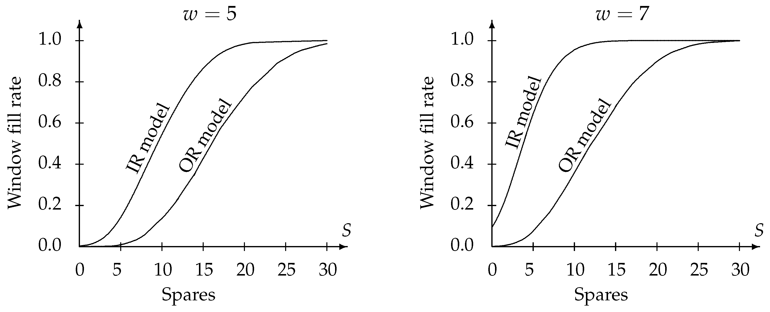
A comparison between the graph of the OR and IR models allows us to determine the cost of outsourcing repairs (compared to in-house repair) in terms of spares needed to maintain a required level of performance. This cost can be deduced from Figure 5 that plots the window fill rates of the IR and OR models against the number of spares when the tolerable wait is $w=5$ (left panel) and $w=10$ (right panel).

In

Table 2. The number of spares required to meet the target window fill rate in each model and the cost of outsourcing.

Tolerable Wait	Spares	${\mathit{WFR}}_{\mathit{t}}=80\%$	${\mathit{WFR}}_{\mathit{t}}=90\%$	${\mathit{WFR}}_{\mathit{t}}=95\%$
$w=2$	OR model	23	32	34
	IR model	20	27	29
	Cost	3	5	5
$w=5$	OR model	22	25	27
	IR model	14	16	18
	Cost	8	9	9
$w=8$	OR model	16	18	21
	IR model	4	5	7
	Cost	12	13	14

Notes: Cost is the difference between the number of spares in the OR model and the number of spares in the IR model.

, we list the numbers of spares that are required to meet common industry performance target levels; $WF{R}_t=80\%,90\%$, and $95\%$, for different values of tolerable waiting. The column in bold in the table is the difference between the two models and represents the cost that we are seeking to determine. For example, when $w=5$ and the required performance level is $WF{R}_t=80\%$, then the OR model dictates that 22 spares must be procured whereas the IR model requires only 14. Therefore, if managers consider outsourcing repair, they must also consider that they will need to augment their stock with eight more spares.

Managerial Implications

Our numerical example illustrates a number of implications that are useful for managers. First, the functional form of the window fill rate in both models is generally S-shaped with the number of spares. That is, when spares are sufficiently low or sufficiently high, adding one more spare offers only a slight improvement. In the former, this is because the system is so short on spares that one more item still leaves it lagging behind. In the latter, the system is so well-off that there is hardly a need for improvement. It is therefore only when the system is somewhere in-between that any additional spare makes an impressional change since it enables the system to serve a large portion of customers on time, something it would not be able to conduct otherwise. Therefore, managers should put checks on the impulse to procure additional spares whenever possible. This should be performed only if the effect of the additional spares will indeed justify their cost, something that heavily depends on the current number of spares in the system.

Second, our sensitivity analysis demonstrates that the window fill rate shifts to the right when the order cycle time increases (Figure 3 and Figure 4) and when the tolerable wait decreases (Figure 5). In other words, if managers have a shortage of spare parts, they must renegotiate contracts for longer service times. Alternatively, managers can offer contracts with shorter service times at a higher premium. The necessary changes to the contract (service times, contract price) can be estimated using our model.

One more implication is with respect to the decision to outsoure repair. As shown in Figure 5, the decision to outsource repairs results in a lower window fill rate. To compensate for this, more spares must be purchased. The cost—in terms of spares—for the baseline case of this decision is demonstrated in Table 2. The most important managerial lesson, therefore, is that while outsourcing has many advantages, managers must keep in mind costs associated with inventory requirements. Our model serves as a tool to make an informed decision about these costs. Furthermore, our baseline example shows that these costs depend very much on the model variables. For example, in the baseline case, the cost of outsourcing is increasing with the tolerable wait and the target performance level.

6. Conclusions

In this paper, we develop the window fill rate formula when item repair is conducted in-house and when repair is outsourced. The difference between the two models is that with in-house repair, items are repaired and returned independently of the other items in the order and therefore an item that was “lucky" to be repaired quickly will return sooner to the system’s stock whilst the other items in its order are still being repaired. In contrast, when repair is outsourced, then it is assumed that when an order for repair is shipped to the external repair firm, then no item will return separately from the other items in the order. Therefore, the system’s stock depends on the longest repair time within each order. Consequently, all else being equal, outsourced repair will result in a lower window fill rate compared to in-house repair.

The derivation of the window fill rate in both models requires tracking the supply of items when the customer demands an item (i.e., w units of time after the customer’s arrival) and the demand of items up to and including the customer’s arrival. In our Poisson demand model, the derivation of the in-house repair formula is quite straightforward since the independence of the delivery times of repaired items implies that these deliveries behave as a Poisson process, too. Therefore, the window fill rate in the in-house repair case can be reduced to a difference between two Poisson processes (i.e., a Skellam random variable) and can be easily computed. In contrast, the derivation of the window fill rate under outsourcing is computationally challenging since items of the same order depend on each other for their delivery.

We overcome this challenge by developing a Monte-Carlo simulation algorithm that considers all the possible delivery states of orders that are relevant to the supply–demand equation. The efficiency of the simulation algorithm stems from the fact that we do not simulate the entire logistical process but instead simulate only the demand arrivals.

We complete our analysis with a numerical illustration that demonstrates the functional form of the window fill rate as a function of the number of spares. The cost of outsourcing repair (in terms of required spares) is discerned by comparing the window fill rate graphs of both models. A manager of a logistic system that considers outsourcing repair must therefore consider how many more spares they will need to procure to maintain the same window fill rate level.

While our model assumes a Poisson demand, our mathematical approach can be used in a similar manner when arrivals follow a compound Poisson process. Unfortunately, for demand that does not follow a Poisson process, deriving a formula for the window fill rate may prove to be too mathematically challenging. Notwithstanding, this study serves even these cases by drawing managers’ attention to the need of adjusting stock levels when conducting organizational changes such as outsourcing repair or establishing in-house repair.

Our model may be extended in a number of ways. As previously stated, our model requires Poisson arrivals and therefore additional research is needed to develop efficient algorithms for estimating the window fill rate in non-Poisson arrival cases. Furthermore, we focus on a single warehouse, whereas large inventory systems employ a network of warehouses with central control of inventory. These systems may be organized in multiple echelons and may provide emergency replenishment from nearby sites. Future work can build on our approach to analyze these complex systems and estimate the optimal number of spares and their allocation.

References

- Wensing, T. Periodic Review Inventory Systems: Lecture Notes in Economics and Mathematical Systems; Springer: New York, NY, USA, 2011; Volume 651. [Google Scholar]
- Ullah, M.; Asghar, I.; Zahid, M.; Omair, M.; AlArjani, A.; Sarkar, B. Ramification of remanufacturing in a sustainable three-echelon closed-loop supply chain management for returnable products. J. Clean. Prod. 2021, 290, 125609. [Google Scholar] [CrossRef]
- Ullah, M.; Sarkar, B. Recovery-channel selection in a hybrid manufacturing-remanufacturing production model with RFID and product quality. Int. J. Prod. Econ. 2020, 219, 360–374. [Google Scholar] [CrossRef]
- Sarkar, B.; Ullah, M.; Sarkar, M. Environmental and economic sustainability through innovative green products by remanufacturing. J. Clean. Prod. 2022, 332, 129813. [Google Scholar] [CrossRef]
- Dreyfuss, M.; Giat, Y. Optimal spares allocation to an exchangeable-item repair system with tolerable wait. Eur. J. Oper. Res. 2017, 261, 584–594. [Google Scholar] [CrossRef]
- Skellam, J.G. The frequency distribution of the difference between two Poisson variates belonging to different populations. J. R. Stat. Soc. Ser. Stat. Soc. 1946, 109, 296. [Google Scholar] [CrossRef]
- Vasilev, J.; Milkova, T. Optimisation Models for Inventory Management with Limited Number of Stock Items. Logistics 2022, 6, 54. [Google Scholar] [CrossRef]
- Scarf, P.; Syntetos, A.; Teunter, R. Joint maintenance and spare-parts inventory models: A review and discussion of practical stock-keeping rules. Ima J. Manag. Math. 2024, 35, 83–109. [Google Scholar] [CrossRef]
- Sherbrooke, C.C. Optimal Inventory Modeling of Systems: Multi-Echelon Techniques; Kluwer: Dordrecht, The Netherlands, 2004; Volume 72. [Google Scholar]
- Muckstadt, J.A. Analysis and Algorithms for Service Parts Supply Chains; Springer Science & Business Media: New York, NY, USA, 2005. [Google Scholar]
- Van Houtum, G.J.; Kranenburg, B. Spare Parts Inventory Control under System Availability Constraints; Springer: New York, NY, USA, 2015; Volume 227. [Google Scholar]
- Basten, R.J.; Ryan, J.K. The value of maintenance delay flexibility for improved spare parts inventory management. Eur. J. Oper. Res. 2019, 278, 646–657. [Google Scholar] [CrossRef]
- Kouki, C.; Larsen, C. Rationing policies in a spare parts inventory system with customers differentiation. Int. J. Prod. Res. 2021, 59, 6270–6290. [Google Scholar] [CrossRef]
- Chen, Y.K.; Gao, Q.; Su, X.B.; Fang, S.; Guo, C.M. Research on optimization of spare parts inventory policy considering maintenance priority. Int. J. Syst. Assur. Eng. Manag. 2018, 9, 1336–1345. [Google Scholar] [CrossRef]
- Sherbrooke, C.C. METRIC: A multi-echelon technique for recoverable item control. Oper. Res. 1968, 16, 122–141. [Google Scholar] [CrossRef]
- Dreyfuss, M.; Giat, Y.; Stulman, A. An analytical approach to determine the window fill rate in a repair shop with cannibalization. Comput. Oper. Res. 2018, 98, 13–23. [Google Scholar] [CrossRef]
- Van Donselaar, K.; Broekmeulen, R.; de Kok, T. Heuristics for setting reorder levels in periodic review inventory systems with an aggregate service constraint. Int. J. Prod. Econ. 2021, 237, 108137. [Google Scholar] [CrossRef]
- Gutierrez, M.; Rivera, F.A. Undershoot and order quantity probability distributions in periodic review, reorder point, order-up-to-level inventory systems with continuous demand. Appl. Math. Model. 2021, 91, 791–814. [Google Scholar] [CrossRef]
- Dehghani, M.; Abbasi, B.; Oliveira, F. Proactive transshipment in the blood supply chain: A stochastic programming approach. Omega 2021, 98, 102112. [Google Scholar] [CrossRef]
- Poormoaied, S. Inventory decision in a periodic review inventory model with two complementary products. Ann. Oper. Res. 2022, 315, 1937–1970. [Google Scholar] [CrossRef]
- Yıldız, B.; Sütçü, M. A variant SDDP approach for periodic-review approximately optimal pricing of a slow-moving a item in a duopoly under price protection with end-of-life return and retail fixed markdown policy. Expert Syst. Appl. 2023, 212, 118801. [Google Scholar] [CrossRef]
- Rodrigues, L.R.; Yoneyama, T. A spare parts inventory control model based on Prognostics and Health monitoring data under a fill rate constraint. Comput. Ind. Eng. 2020, 148, 106724. [Google Scholar] [CrossRef]
- Giat, Y. Allocation of scarce resources in a network with periodic deliveries and customer tolerable wait. Comput. Ind. Eng. 2021, 159, 107462. [Google Scholar] [CrossRef]
- Baloch, G.; Gzara, F. Inventory planning for self-serve pharmacy kiosks: A fill rate maximization approach. Comput. Ind. Eng. 2024, 188, 109836. [Google Scholar] [CrossRef]
- Lamghari-Idrissi, D.; Basten, R.; van Houtum, G.J. Spare parts inventory control under a fixed-term contract with a long-down constraint. Int. J. Prod. Econ. 2020, 219, 123–137. [Google Scholar] [CrossRef]
- Durrande-Moreau, A. Waiting for service: Ten years of empirical research. Int. J. Serv. Ind. Manag. 1999, 10, 171–194. [Google Scholar] [CrossRef]
- Atkinson, M.; Ntontis, E.; Neville, F.; Reicher, S. “I’ll wait for the English one”: COVID-19 vaccine country of origin, national identity, and their effects on vaccine perceptions and uptake willingness. Soc. Personal. Psychol. Compass 2023, 17, e12837. [Google Scholar] [CrossRef]
- Drabicki, A.; Cats, O.; Kucharski, R.; Fonzone, A.; Szarata, A. Should I stay or should I board? Willingness to wait with real-time crowding information in urban public transport. Res. Transp. Bus. Manag. 2023, 47, 100963. [Google Scholar] [CrossRef]
- Feng, B.; Fan, Z.P.; Li, Y. A decision method for supplier selection in multi-service outsourcing. Int. J. Prod. Econ. 2011, 132, 240–250. [Google Scholar] [CrossRef]
- Hathaway, B.A.; Emadi, S.M.; Deshpande, V. Personalized priority policies in call centers using past customer interaction information. Manag. Sci. 2022, 68, 2806–2823. [Google Scholar] [CrossRef]
- Caggiano, K.E.; Jackson, P.L.; Muckstadt, J.A.; Rappold, J.A. Efficient computation of time-based customer service levels in a multi-item, multi-echelon supply chain: A practical approach for inventory optimization. Eur. J. Oper. Res. 2009, 199, 744–749. [Google Scholar] [CrossRef]
- Dreyfuss, M.; Giat, Y. Optimal allocation of spares to maximize the window fill rate in a two-echelon exchangeable-item repair system. Eur. J. Oper. Res. 2018, 270, 1053–1062. [Google Scholar] [CrossRef]
- Dreyfuss, M.; Giat, Y. The window fill rate with nonzero assembly times: Application to a battery swapping network. In Proceedings of the Operations Research and Enterprise Systems: 6th International Conference, ICORES 2017, Porto, Portugal, 23–25 February 2017; Revised Selected Papers 6. Springer: Berlin/Heidelberg, Germany, 2018; pp. 42–62. [Google Scholar]
- Yang, J.; Liu, W.; Ma, K.; Yue, Z.; Zhu, A.; Guo, S. An optimal battery allocation model for battery swapping station of electric vehicles. Energy 2023, 272, 127109. [Google Scholar] [CrossRef]
- Xu, Y.; Serel, D.A.; Bisi, A.; Dada, M. Setting fulfillment-time guarantees for accepting customer orders in a periodic-review base-stock inventory system. IISE Trans. 2023, 1–14. [Google Scholar] [CrossRef]
- Van der Heijden, M.C.; De Kok, A. Customer waiting times in an (R, S) inventory system with compound Poisson demand. Z. FÜR Oper. Res. 1992, 36, 315–332. [Google Scholar]
- Dreyfuss, M.; Giat, Y. Allocating spares to maximize the window fill rate in a periodic review inventory system. Int. J. Prod. Econ. 2019, 214, 151–162. [Google Scholar] [CrossRef]
- Giat, Y.; Dreyfuss, M. The window fill rate in a periodic review inventory system with order crossover. Int. J. Prod. Res. 2021, 59, 6791–6808. [Google Scholar] [CrossRef]
- Bouhnik, D.; Giat, Y. ISO 9001 as a tool for improving knowledge management in business ecosystems. Int. J. Knowl. Based Dev. 2015, 6, 261–272. [Google Scholar] [CrossRef]
- Öztürk, H. A deterministic economic production quantity model with partial backordering and outsourcing repair of non-conforming products. Int. J. Syst. Sci. Oper. Logist. 2022, 9, 355–383. [Google Scholar] [CrossRef]
- Driessen, M.; Arts, J.; van Houtum, G.J.; Rustenburg, J.W.; Huisman, B. Maintenance spare parts planning and control: A framework for control and agenda for future research. Prod. Plan. Control. 2015, 26, 407–426. [Google Scholar] [CrossRef]
- Basten, R.J.; van der Heijden, M.C.; Schutten, J.M. Practical extensions to a minimum cost flow model for level of repair analysis. Eur. J. Oper. Res. 2011, 211, 333–342. [Google Scholar] [CrossRef]
- Hallak, B.K.; Nasr, W.W.; Jaber, M.Y. Re-ordering policies for inventory systems with recyclable items and stochastic demand–Outsourcing vs. in-house recycling. Omega 2021, 105, 102514. [Google Scholar] [CrossRef]
- Benmoussa, O. Improving Replenishment Flows Using Simulation Results: A Case Study. Logistics 2022, 6, 34. [Google Scholar] [CrossRef]
- Papaleonidas, C.; Androulakis, E.; Lyridis, D.V. A Simulation-based planning tool for floating storage and regasification units. Logistics 2020, 4, 31. [Google Scholar] [CrossRef]
- Sarkar, A.; Guchhait, R.; Sarkar, B. Application of the artificial neural network with multithreading within an inventory model under uncertainty and inflation. Int. J. Fuzzy Syst. 2022, 24, 2318–2332. [Google Scholar] [CrossRef]
- Sarkar, B.; Tayyab, M.; Kim, N.; Habib, M.S. Optimal production delivery policies for supplier and manufacturer in a constrained closed-loop supply chain for returnable transport packaging through metaheuristic approach. Comput. Ind. Eng. 2019, 135, 987–1003. [Google Scholar] [CrossRef]
Figure 1.
Time axes of demand and supply when arrival is early and late in the cycle. is all the customers that arrived until the arrow’s tail plus the item required by Jane. is S plus all the items that were repaired until the arrowhead.
Figure 2.
The relevant orders after re-indexing. When Jane arrived early in the cycle, then any order prior to order is surely delivered on time and is therefore irrelevant. In contrast, when Jane arrived late in the cycle, then also order is surely delivered on time and is irrelevant.
Figure 3.
The window fill rate as a function of the spares when repair is in-house (IR model) for different values of cycle time. The other parameters’ values are when , , and . The dotted line expresses the number of spares needed to maintain an 80% window fill rate.
Figure 4.
The window fill rate as a function of the spares when repair is outsourced (OR model) for different values of cycle time. The other parameters’ values are when , , and . The dotted line expresses the number of spares needed to maintain an 80% window fill rate.
Figure 5.
The window fill rate as a function of the spares when repair is in-house (IR model). In the left panel, the tolerable wait is and in the right panel, the tolerable wait is . The other parameters’ values are , , and .