Water-Air Volatilization Factors to Determine Volatile Organic Compound (VOC) Reference Levels in Water


Abstract
:
1. Introduction
2. Methodology
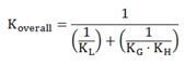
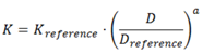
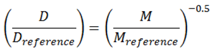
2.1. Mass Transfer Coefficients

| Geometry | KL (m∙s−1) | KG (m∙s−1) | ||
|---|---|---|---|---|
| Flat [6] (p. 915) | 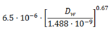 | (4) | 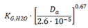 u = 0, KG,H2O = 3 × 10⁻³ m·s−1 u = 2.25 m·s−1, KG,H2O = 8.5 × 10⁻³ m·s−1 | (5) |
| Sphere [7,10,11] (p. G-2) | 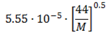 | (6) |  | (7) |
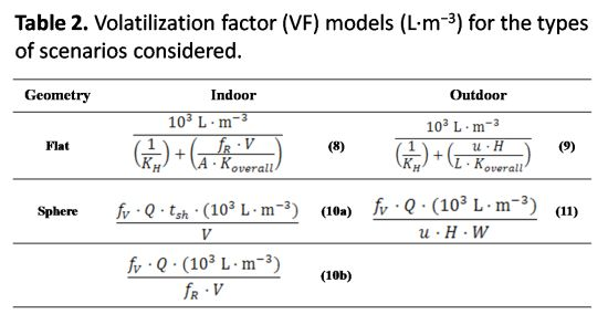
2.2. Summary of VFs
| Geometry | Indoor | Outdoor | ||
|---|---|---|---|---|
| Flat | 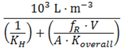 | (8) |  | (9) |
| Sphere |  | (10a) | 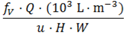 | (11) |
 | (10b) | |||
2.3. Application to a Case Study
| SCENARIOS | Vegetable | Water | Air | |||
|---|---|---|---|---|---|---|
| Ingestion | Ingestion | Dermal Contact | Inhalation Indoor | Inhalation Outdoor | ||
| E1A | Crop Consumption | Irrigated | ||||
| E1B | Indoor irrigation (e.g., greenhouse) | Irrigated | direct | Sprinkler (sphere) | ||
| E1C | Exterior irrigation (inundation and sprinkler) | Irrigated | direct | Sprinkler (sphere) Puddle (flat) | ||
| E2A | Personal hygiene (shower and hand cleaning) | direct | direct | Shower (sphere) | ||
| E2B | Industrial cleaning (e.g., cleaning pools) | direct | From pool (flat) Sprinkler (sphere) | |||
| E3A | Domestic hygiene (shower and hand cleaning) | direct | direct | Shower (sphere) | ||
| E3B | Private gardens (irrigation with sprinkler) | direct | direct | Sprinkler (sphere) | ||
| E4A | Street cleaning (sprinkler) | direct | Sprinkler (sphere) | |||
| E4B | Urban cleaning (sprinkler) | direct | Sprinkler (sphere) | |||
| E5A | Recreational bath (pools ) | direct | direct | From pool (flat) | ||
| Parameter | E1B | E2A | E2B Flat | E2B sph/E4B | E3A | E5A | Reference |
|---|---|---|---|---|---|---|---|
| fR (s−1) | 2.3 × 10⁻³ | - | 2.3 × 10⁻³ | 2.3 × 10⁻³ | - | 1.4 × 10⁻³ | [5] (p. 28) |
| V (m3) | 300 | 4.5 | - | 1250 | 4.5 | - | Calculated |
| V/A (m) | - | - | 3 | - | - | 2 | [5] (p. 28) |
| ttravel (s) | 10 | 0.64 | - | 0.64 | 0.64 | - | [12] |
| d (m) | 2 × 10⁻³ | 2 × 10⁻³ | - | 2 × 10⁻³ | 1 × 10⁻³ | - | [12] |
| Q·105 (m3·s−1) | 5.55 | 16.6 | - | 50 | 16.6 | - | [7,12] |
| tsh (s) | - | 600 | - | - | 600 | - | [9] |
| Parameter | E1C Flat | E1C sph | E3B | E4A | References |
|---|---|---|---|---|---|
| u (m·s−1) | 2.25 | 2.25 | 2.25 | 2.25 | [5] (p. 28) |
| H (m) | 1.5 | 2.5 | 2 | 2 | [5] (p. 28) and calculated |
| L (m) | 15 | - | - | - | [5] (p. 28) |
| ttravel (s) | - | 10 | 0.64 | 0.64 | [12] |
| d (m) | - | 2 × 10⁻³ | 2 × 10⁻³ | 2 × 10⁻³ | [12] |
| Q·105 (m3·s−1) | - | 50 | 50 | 183 | [7,12] |
| W (m) | - | 18 | 8 | 8 | Local data |
| M (g·mole−1) | KH | Da (m2·s−1) | Dw (m2·s−1) | Rank KH | |
|---|---|---|---|---|---|
| Acetone | 5.81 × 101 | 1.62 × 10⁻³ | 1.24 × 10⁻⁵ | 1.14 × 10⁻⁹ | 2 |
| Benzene | 7.81 × 101 | 2.27 × 10⁻¹ | 8.80 × 10⁻⁶ | 9.80 × 10⁻¹⁰ | 18 |
| Bromoform | 2.53 × 10² | 2.19 × 10⁻² | 1.49 × 10⁻⁶ | 1.03 × 10⁻⁹ | 7 |
| Butanone, 2- | 7.21 × 101 | 2.33 × 10⁻³ | 8.08 × 10⁻⁶ | 9.86 × 10⁻¹⁰ | 3 |
| Carbon Tetrachloride | 1.54 × 10² | 1.13 × 100 | 7.30 × 10⁻⁶ | 8.70 × 10⁻¹⁰ | 29 |
| Chlorobenzene | 1.13 × 10² | 1.27 × 10⁻¹ | 1.04 × 10⁻⁵ | 1.00 × 10⁻⁹ | 13 |
| Chloroform | 1.19 × 10² | 1.50 × 10⁻¹ | 1.04 × 10⁻⁵ | 9.90 × 10⁻¹⁰ | 15 |
| Dichloroethylene, 1,1 | 9.69 × 101 | 1.07 × 100 | 1.01 × 10⁻⁵ | 1.17 × 10⁻⁹ | 28 |
| Dichloroethylene, c-1,2 | 9.69 × 101 | 1.67 × 10⁻¹ | 9.00 × 10⁻⁶ | 1.04 × 10⁻⁹ | 16 |
| Dichloromethane | 8.49 × 101 | 1.33 × 10⁻¹ | 7.36 × 10⁻⁶ | 1.13 × 10⁻⁹ | 14 |
| Dichloromethane, 1,2 | 9.90 × 101 | 4.82 × 10⁻² | 7.07 × 10⁻⁶ | 1.19 × 10⁻⁹ | 10 |
| Dichloroethylene, t-1,2 | 9.69 × 101 | 3.83 × 10⁻¹ | 6.95 × 10⁻⁶ | 7.34 × 10⁻¹⁰ | 24 |
| ETBE | 1.02 × 10² | 9.99 × 10⁻² | 7.50 × 10⁻⁶ | 7.80 × 10⁻¹⁰ | 12 |
| Ethylbenzene | 1.06 × 10² | 3.22 × 10⁻¹ | 1.78 × 10⁻⁵ | 1.98 × 10⁻⁹ | 23 |
| Formaldehyde | 3.00 × 101 | 1.38 × 10⁻⁵ | 5.42 × 10⁻⁶ | 5.91 × 10⁻¹⁰ | 1 |
| Hexachlorobenzene | 2.85 × 10² | 6.95 × 10⁻² | 7.92 × 10⁻⁶ | 9.41 × 10⁻⁹ | 11 |
| MTBE | 8.81 × 101 | 2.44 × 10⁻² | 5.90 × 10⁻⁶ | 7.50 × 10⁻¹⁰ | 8 |
| Naphthalene | 1.28 × 10² | 1.80 × 10⁻² | 7.10 × 10⁻⁶ | 7.90 × 10⁻¹⁰ | 6 |
| Tetrachloroethane | 1.68 × 10² | 1.50 × 10⁻² | 7.20 × 10⁻⁶ | 8.20 × 10⁻¹⁰ | 5 |
| Tetrachloroethylene | 1.66 × 10² | 7.24 × 10⁻¹ | 7.80 × 10⁻⁶ | 8.80 × 10⁻¹⁰ | 27 |
| Tetrahydrofuran | 7.21 × 101 | 5.75 × 10⁻³ | 9.30 × 10⁻⁶ | 9.88 × 10⁻¹⁰ | 4 |
| Toluene | 9.21 × 101 | 2.71 × 10⁻¹ | 8.70 × 10⁻⁶ | 8.60 × 10⁻¹⁰ | 19 |
| Trichloroethane, 1,1,1 | 1.33 × 10² | 7.03 × 10⁻¹ | 7.80 × 10⁻⁶ | 8.80 × 10⁻¹⁰ | 26 |
| Trichloroethane, 1,1,2 | 1.33 × 10² | 3.37 × 10⁻² | 7.80 × 10⁻⁶ | 8.80 × 10⁻¹⁰ | 9 |
| Trichloroethylene | 1.31 × 10² | 4.03 × 10⁻¹ | 7.90 × 10⁻⁶ | 9.10 × 10⁻¹⁰ | 25 |
| Trichlorofluoromethane | 1.37 × 10² | 3.97 × 100 | 8.70 × 10⁻⁶ | 9.70 × 10⁻¹⁰ | 30 |
| xylene, m- | 1.06 × 10² | 2.94 × 10⁻¹ | 7.00 × 10⁻⁶ | 7.80 × 10⁻¹⁰ | 22 |
| xylene, o- | 1.06 × 10² | 2.12 × 10⁻¹ | 8.70 × 10⁻⁶ | 1.00 × 10⁻⁹ | 17 |
| xylene, p- | 1.06 × 10² | 2.82 × 10⁻¹ | 7.69 × 10⁻⁶ | 8.44 × 10⁻¹⁰ | 21 |
| xylenes (average) | 1.06 × 10² | 2.71 × 10⁻¹ | 7.14 × 10⁻⁶ | 9.34 × 10⁻¹⁰ | 20 |
3. Results and Discussion
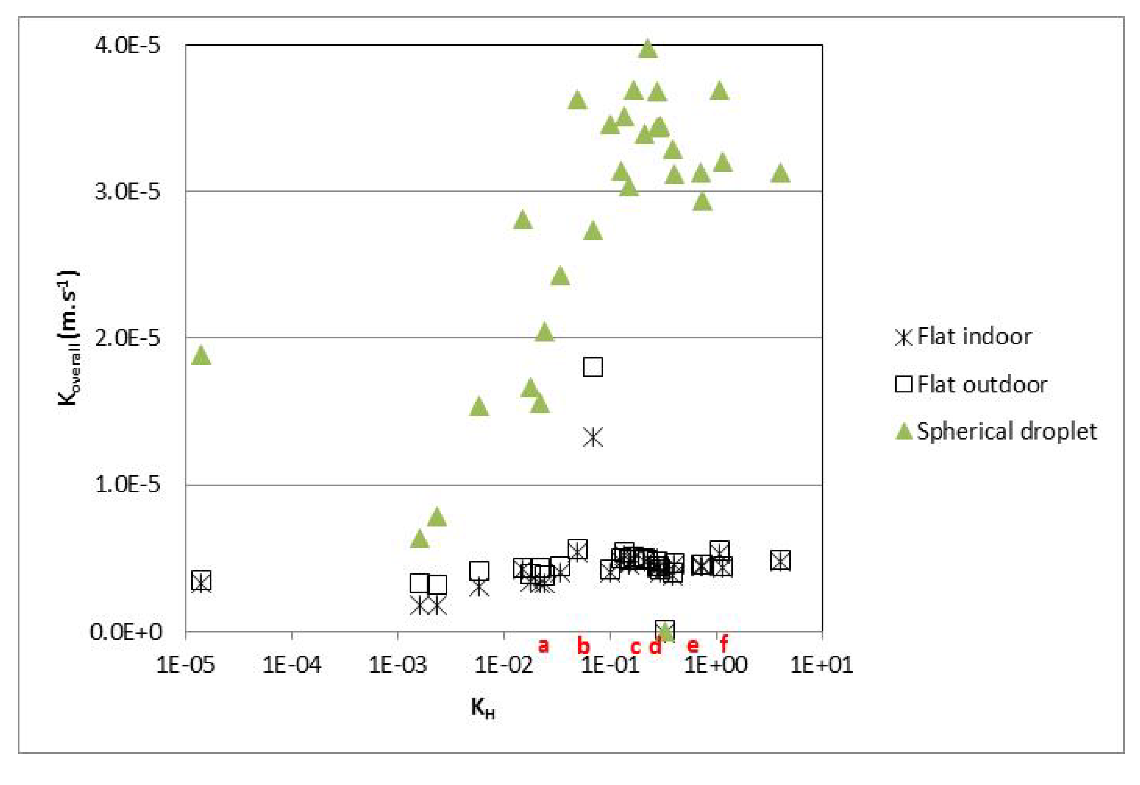
3.1. Mass-Transfer Coefficients

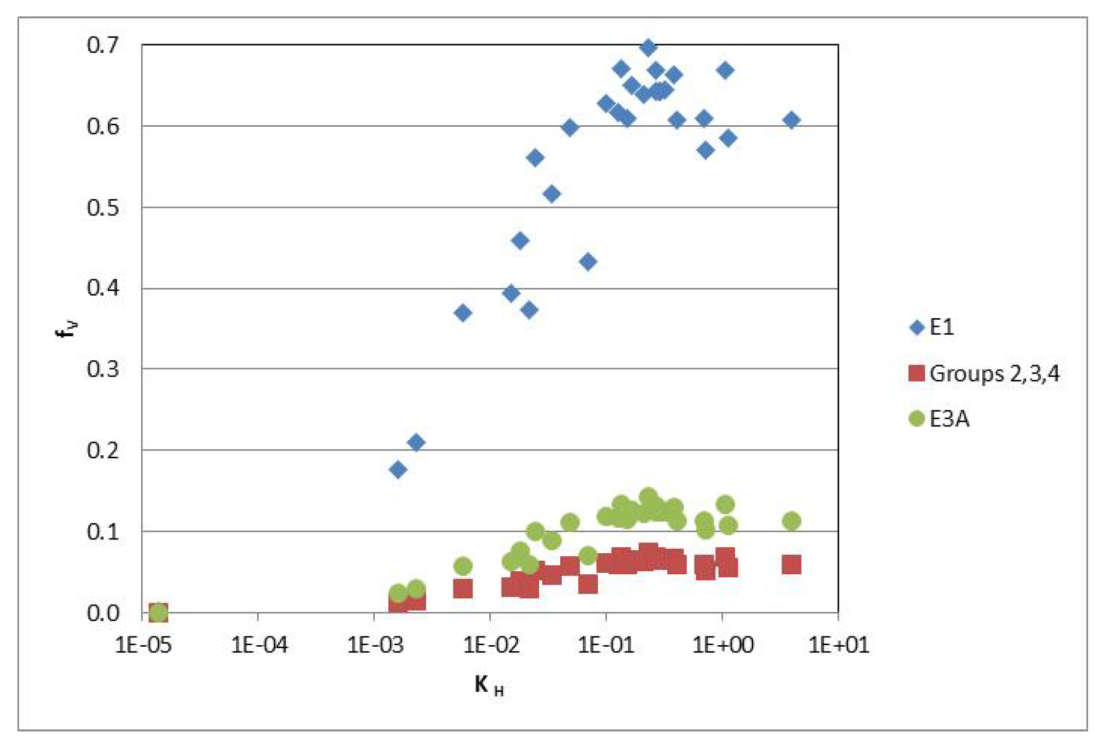
3.2. Fraction of Volatilization
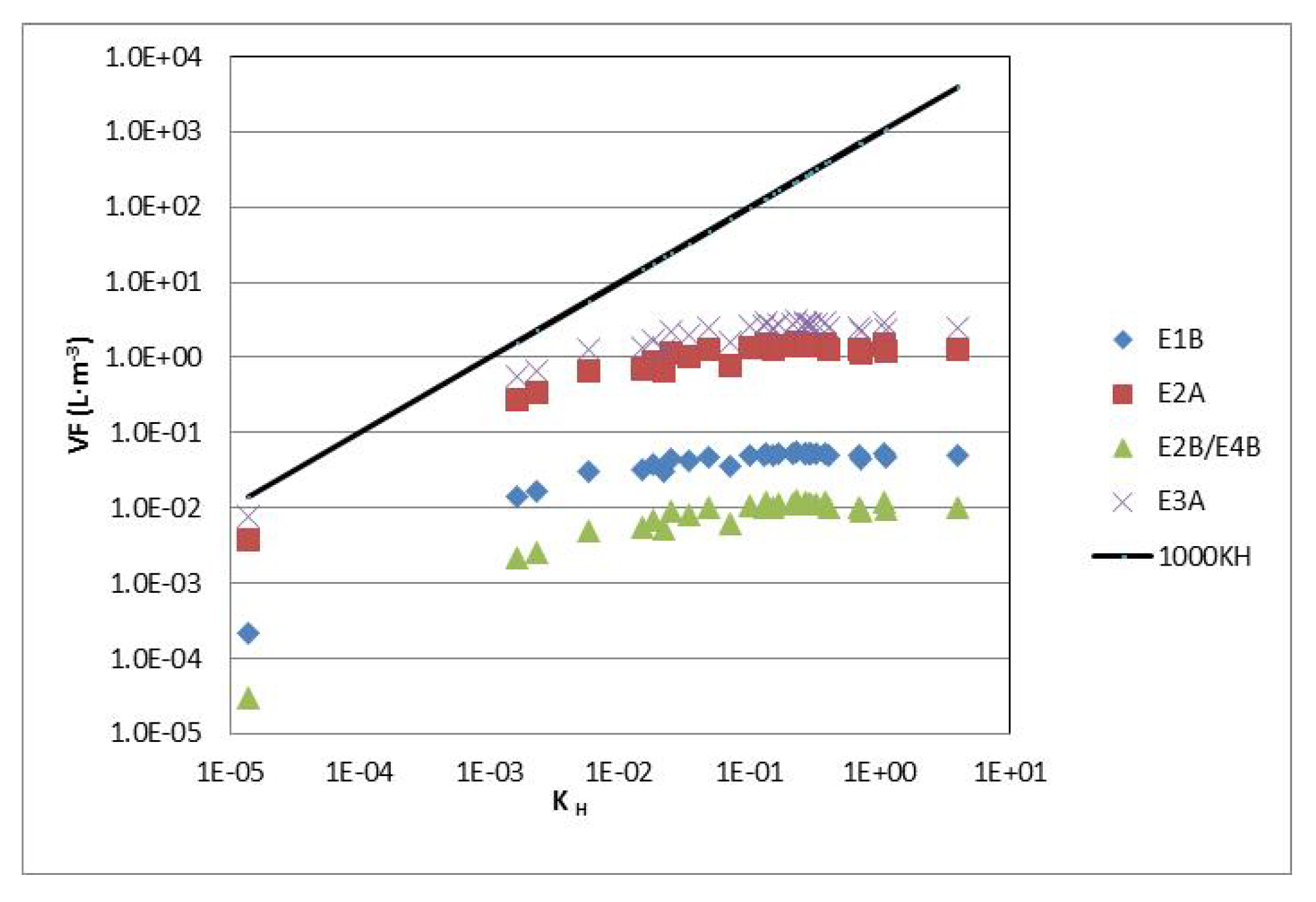
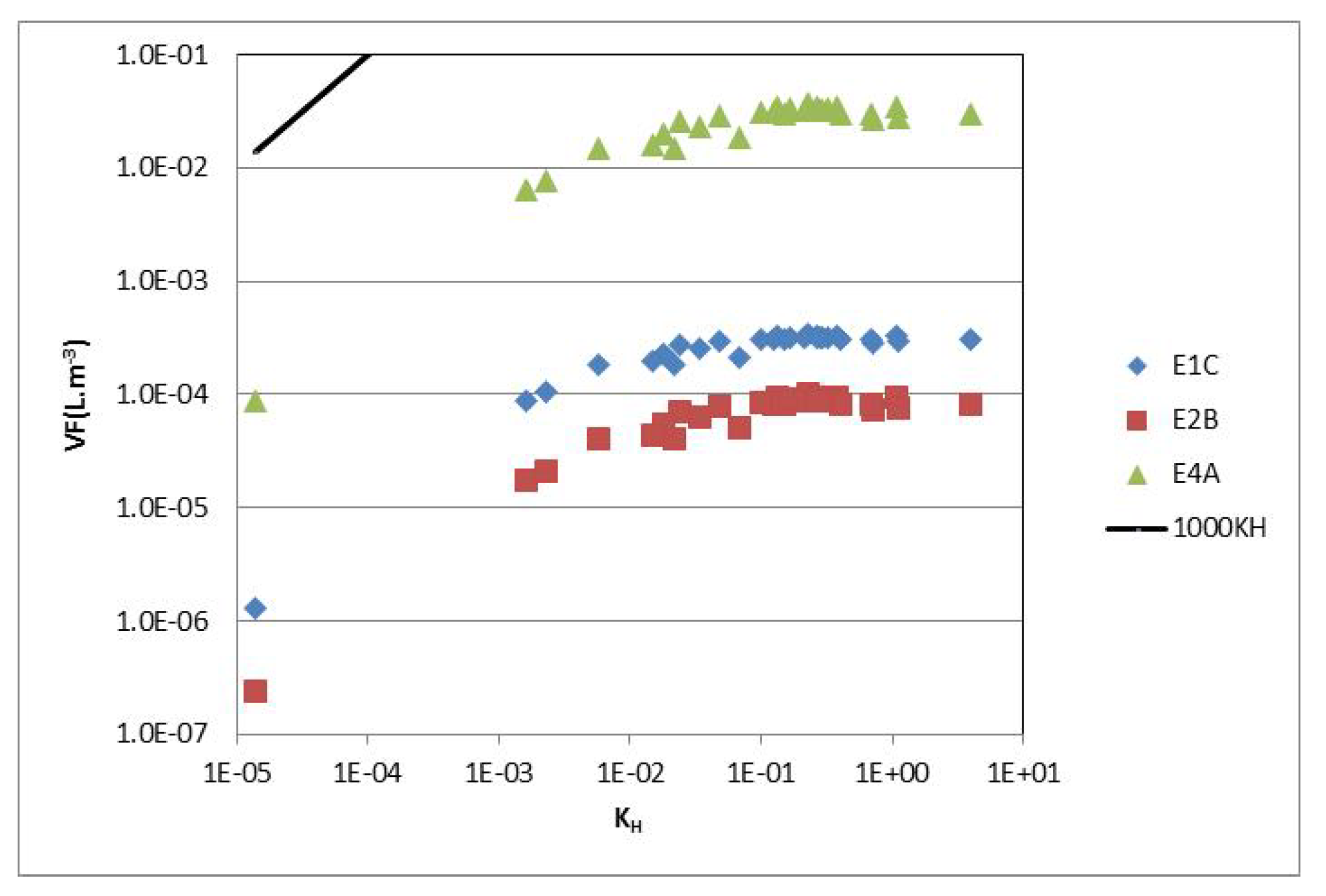
3.3. VFs for Flat Geometries

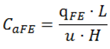
3.4. VFs for Spherical Geometries


3.5. Comparison with Experimental/Real VFs Values
| T (°C) | Model, Scenarios Representative | VF (L·m−3) | fV | n | Refs. | |
|---|---|---|---|---|---|---|
| Acetone | 23–24 | Flat, E2B, E5A | 0.44–0.46 | 0.049–0.058 | 2 | [18] |
| Toluene | 23–24 | Flat, E2B, E5A | 3.6–5 | 0.29–0.31 | 2 | [18] |
| Ethylbenzene | 23–24 | Flat, E2B, E5A | 3.1–4.6 | 0.31–0.33 | 2 | [18] |
| Chloroform | 20–30 | Flat, E2B, E5A | 1.4–21.4 | - | 4–70 | [17,19,20,21,22] |
| Acetone | 21–22 | Drop, E2A, E3A | 0.83–1.3 | 0.063–0.093 | 4 | [23] |
| Ethylbenzene | 21–23 | Drop, E2A, E3A | 1.5–4.8 | 0.58–0.63 | 4 | [23] |
| Toluene | 21–24 | Drop, E2A, E3A | 4.1–9.1 | 0.58–0.64 | 4 | [23] |
| Trichloroethylene | 21–27 | Drop, E2A, E3A | 15–88 | 0.44–0.57 | 4 | [24] |
| Chloroform | 26–29 | Drop, E2A, E3A | 3.5–18 | 0.46–0.52 | 4 | [24] |
| Trichloroethylene | 21–22 | Drop, E2A, E3A | 54–103 | 0.50–0.67 | 2 | [25] |
4. Conclusions
Acknowledgments
Author Contributions
Appendix—Theoretical Expressions for VFs (Table 2)
A.1. Flat Surface


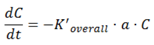
A.2. Spherical Droplets


Conflicts of Interest
References
- United States Environmental Protection Agency (USEPA). Risk Assessment Guidance for Superfund: Volume 1—Human Health Evaluation Manual (Part B, Development of Risk-based Preliminary Remediation Goals); EPA/540/R-92/003; USEPA: Washington, DC, USA, 1991.
- European Commission. Technical Guidance Document on Risk Assessment in Support of Commission Directive 93/67/EEC on Risk Assessment for New Notified Substances, Commission Regulation (EC) No 1488/94 on Risk Assessment for Existing Substances and Directive 98/8/EC of the European Parliament and of the Council Concerning the Placing of Biocidal Products on the Market, Part I; European Commission Joint Research Centre: Brussels, Belgium, 2007. [Google Scholar]
- Risk Assessment Information System (RAIS). Available online: http://rais.ornl.gov/cgi-bin/prg/PRG_search?select=chem (accessed on 27 March 2014).
- Orejudo, E.; Mora, R.; Carnicero, V.; Martí, V.; López, D.; de Pablo, J.; Rovira, M. Development of risk-based contaminant reference concentration based on protection of human health for the sustainable use of groundwater. In Proceedings of the Consoil 2008, 10th International UFZ/TNO Conference on Soil-Water Systems, Milano, Italy, 3–6 June 2008.
- American Society for Testing Materials. In Standards Guide for Risk-Based Corrective Action Applied at Pretroleum Release Sites; E1739-95; ASTM: West Conshohocken, PA, USA, 1995.
- Schwarzenbach, R.P.; Gschwend, P.M.; Imboden, D.M. Environmental Organic Chemistry, 2nd ed.; Wiley Interscience: New York, NY, USA, 2003. [Google Scholar]
- Waterloo Hydrogeologic Inc. Risc WorkBench User’s Manual: Human Health Risk Assessment Software for Contaminated Sites. v.4.0.; WHI: Waterloo, ON, Canada, 2001. [Google Scholar]
- Orejudo, E.; Mora, R.; Carnicero, V.; Martí, V.; López, D.; de Pablo, J.; Rovira, M. Simplified methodology for the sensitivity analysis of guideline values applied to water. D- Risks & Impacts. In Proceedings of the Consoil 2008, 10th International UFZ/TNO Conference on Soil-Water Systems, Milano, Italy, 3–6 June 2008.
- United States Environmental Protection Agency (USEPA). Water Quality Assessment, a Screening Procedure for Toxic and Conventional Pollutants in Surface and Ground Water (Part I); EPA/600/6-85/002a; USEPA: Washington, DC, USA, 1985.
- Foster, S.A.; Chrostowski, P.C. Integrated Household Exposure Model for Use of Tap Water Contaminated with Volatile Organic Chemicals. In Proceedings of the 79th Annual Meeting of the Air Pollution Control Association, Minneapolis, MN, USA, 22–27 June 1986.
- Carver, J.H.; Seigneur, C.S.; Block, R.M.; Miller, T.M. Comparison of Exposure Models for Volatile Organics in Tap Water. In Proceedings of Eighth Annual Hazmacon. Santa Clara, CA, USA, 15–18 April 1991.
- Walden, J.A.; Spence, L.R. Risk-Based BTEX Screening Criteria for a Groundwater Irrigation Scenario. J. Hum. Ecol. Risk Assess. 1997, 3, 699–722. [Google Scholar] [CrossRef]
- Risk Assessment Information System (RAIS). Available online: http://rais.ornl.gov/cgi-bin/tools/TOX_search?select=chem_spef (accessed on 30 May 2006).
- GSI Environmental, GSI Chemical Properties Database. Available online: http://www.gsi-net.com/es/publicaciones/gsi-chemical-database/list.html (accessed on 30 May 2006).
- Andelman, J.B. Total Exposure to Volatile Organic Compounds in Potable Water. In Significance and Treatment of Volatile Organic Compounds in Water Supplies; Lewis Publishers: Chelsea, MI, USA, 1990; Chapter 20; pp. 485–504. [Google Scholar]
- United States Environmental Protection Agency (USEPA). Volatilization Rates from Water to Indoor Air—Phase II; EPA 600/R-00/096; USEPA; USEPA: Washington, DC, USA, 2000.
- Lourencetti, C.; Grimalt, J.O.; Marco, E.; Fernandez, P.; Font-Ribera, L.; Villanueva, C.M.; Kogevinas, M. Trihalomethanes in chlorine and bromine disinfected swimming pools: Air-water distributions and human exposure. Environ. Int. 2012, 45, 59–67. [Google Scholar]
- Howard, C.L. Volatilization Rates of Chemicals from Drinking Water to Indoor Air. Ph.D. Dissertation, The University of Texas , Austin, TX, USA, 1998. [Google Scholar]
- Aggazzotti, G.; Fantuzzi, G.; Righi, E.; Predieri, G. Environmental and biological monitoring of chloroform in indoor swimming pools. J. Chromatogr. A 1995, 710, 181–190. [Google Scholar] [CrossRef]
- Aggazzotti, G.; Fantuzzi, G.; Righi, E.; Predieri, G. Blood and breath analyses as biological indicators of exposure to trihalomethanes in indoor swimming pools. Sci. Total Environ. 1998, 217, 155–163. [Google Scholar] [CrossRef]
- Fantuzzi, G.; Righi, E.; Predieri, G.; Ceppelli, G.; Gobba, F.; Aggazzotti, G. Occupational exposure to trihalomethanes in indoor swimming pools. Sci. Total Environ. 2001, 264, 257–265. [Google Scholar] [CrossRef]
- Caro, J.; Gallego, M. Assessment of exposure of workers and swimmers to trihalomethanes in an indoor swimming pool. Environ. Sci. Technol. 2007, 41, 4793–4798. [Google Scholar] [CrossRef]
- Moya, J.; Howard-Reed, C.; Corsi, R.L. Volatilization of chemicals from tap water to indoor air from contaminated water used for showering. Environ. Sci. Technol. 1999, 33, 2321–2327. [Google Scholar] [CrossRef]
- Giardino, N.J.; Andelman, J.B. Characterization of the emission of trichloroethylene, chloroform and 1,2-dibromo-3-chloropropsne in a full-size experimental shower. J. Expo. Anal. Environ. Epidemiol. 1996, 6, 413–423. [Google Scholar]
- Giardino, N.J.; Esmen, N.A.; Andelman, J.B. Modeling volatilization of trichloroethylene from a domestic shower spray: The role of drop-size distribution. Environ. Sci. Technol. 1992, 26, 1602–1606. [Google Scholar] [CrossRef]
© 2014 by the authors; licensee MDPI, Basel, Switzerland. This article is an open access article distributed under the terms and conditions of the Creative Commons Attribution license (http://creativecommons.org/licenses/by/3.0/).
Share and Cite
Martí, V.; De Pablo, J.; Jubany, I.; Rovira, M.; Orejudo, E. Water-Air Volatilization Factors to Determine Volatile Organic Compound (VOC) Reference Levels in Water. Toxics 2014, 2, 276-290. https://doi.org/10.3390/toxics2020276
Martí V, De Pablo J, Jubany I, Rovira M, Orejudo E. Water-Air Volatilization Factors to Determine Volatile Organic Compound (VOC) Reference Levels in Water. Toxics. 2014; 2(2):276-290. https://doi.org/10.3390/toxics2020276
Chicago/Turabian StyleMartí, Vicenç, Joan De Pablo, Irene Jubany, Miquel Rovira, and Emili Orejudo. 2014. "Water-Air Volatilization Factors to Determine Volatile Organic Compound (VOC) Reference Levels in Water" Toxics 2, no. 2: 276-290. https://doi.org/10.3390/toxics2020276
APA StyleMartí, V., De Pablo, J., Jubany, I., Rovira, M., & Orejudo, E. (2014). Water-Air Volatilization Factors to Determine Volatile Organic Compound (VOC) Reference Levels in Water. Toxics, 2(2), 276-290. https://doi.org/10.3390/toxics2020276