
Assessing the Water Pollution of the Brahmaputra River Using Water Quality Indexes


Abstract
:1. Introduction
- The intensification of the eutrophication process;
- The availability of dissolved oxygen;
- The health assessment of the ecosystems;
- The specific physical and chemical processes occurring in the evaluated water bodies.
2. Material and Methods
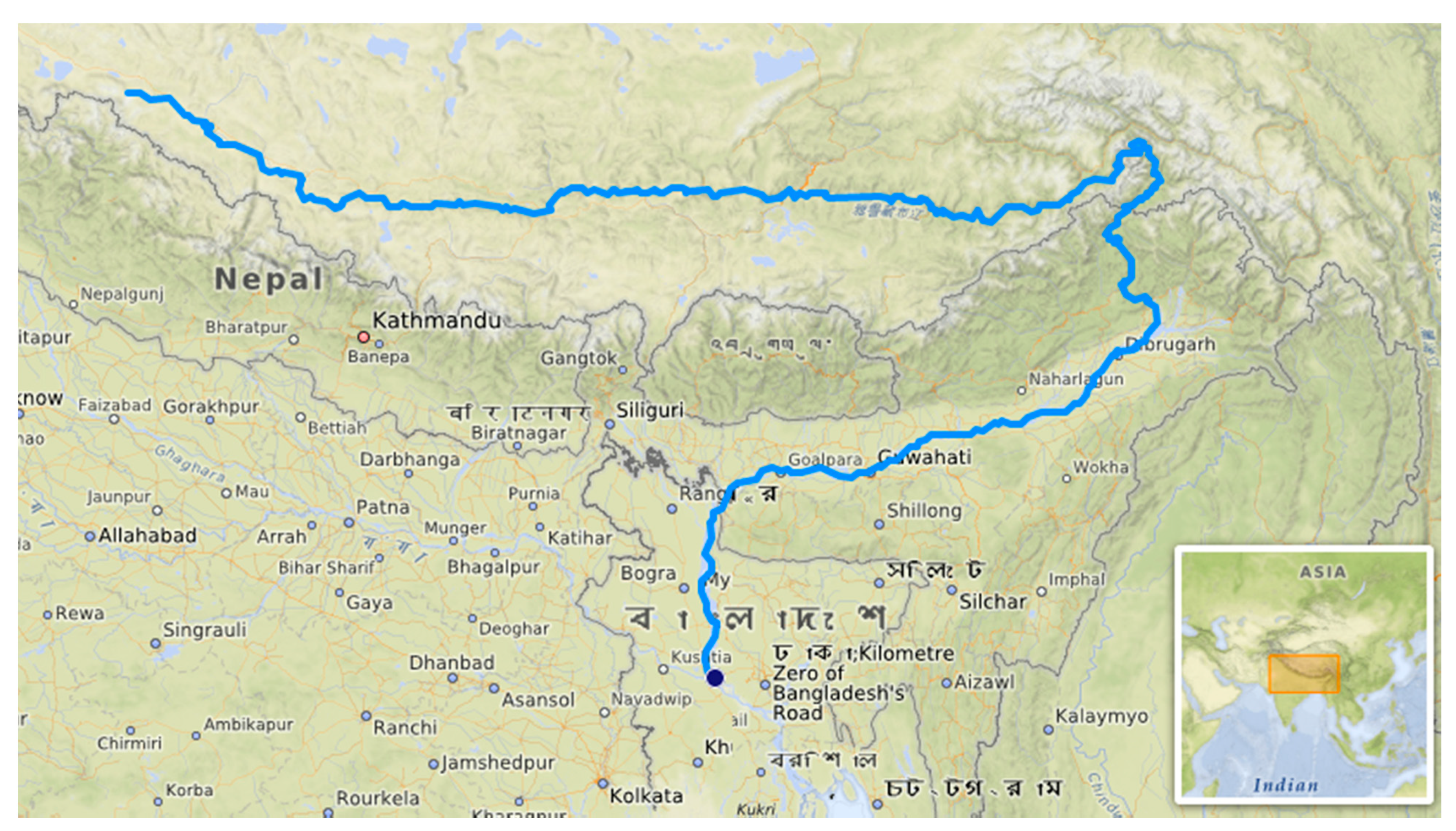
2.1. Study Area and Data Series
2.2. Preliminary Statistical Analyses
2.3. The Water Pollution Indices
- (a)
- F1 is the ratio between the number of the failed parameters and the total number of parameters, multiplied by 100;
- (b)
- F2 is the ratio between the number of the failed tests and the total number of tests, multiplied by 100.
2.4. Classification
2.5. Determination of the WQI Trend in Time and over the Region
3. Results and Discussion
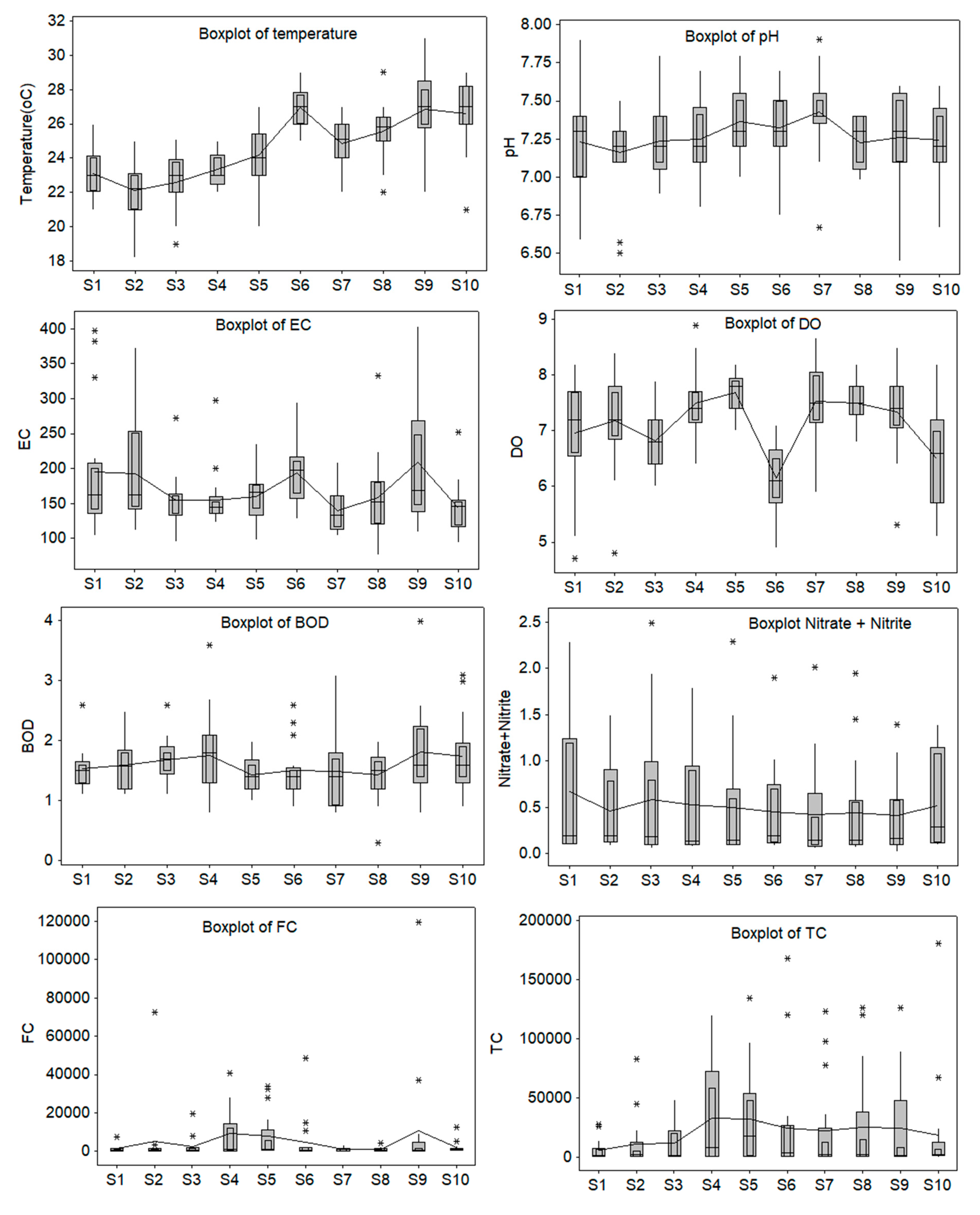
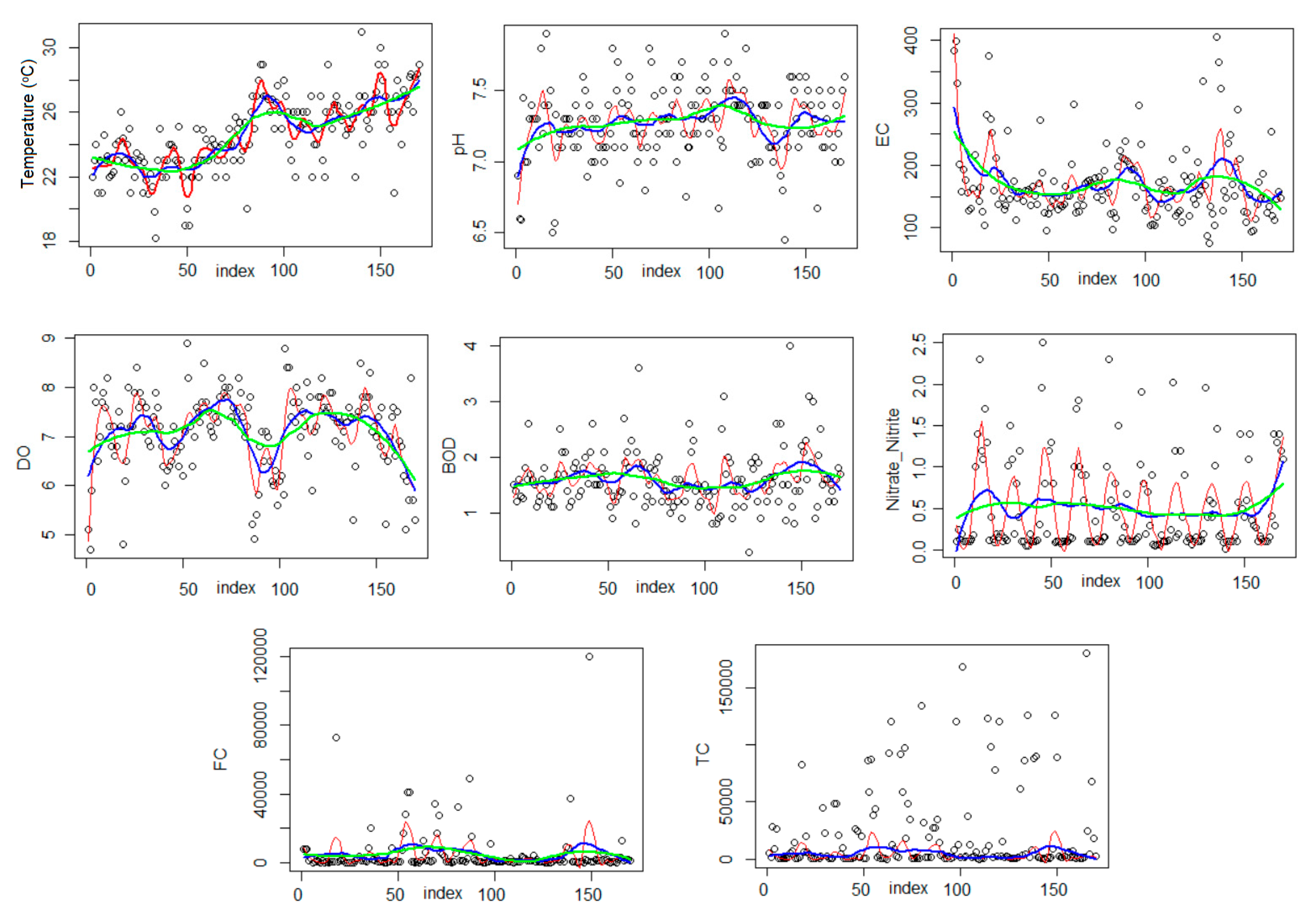
3.1. Statistical Analysis
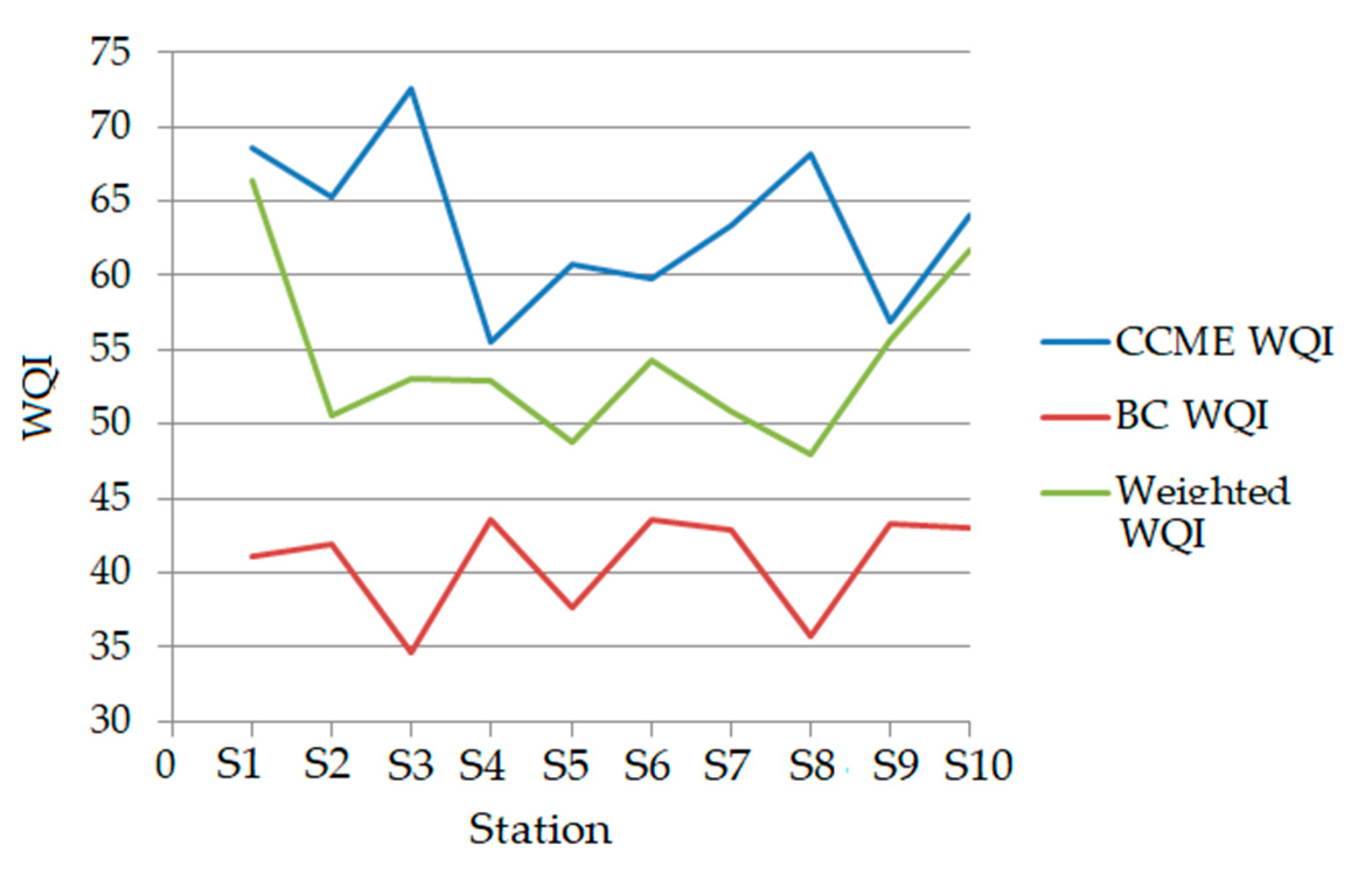
3.2. WQIs Computation
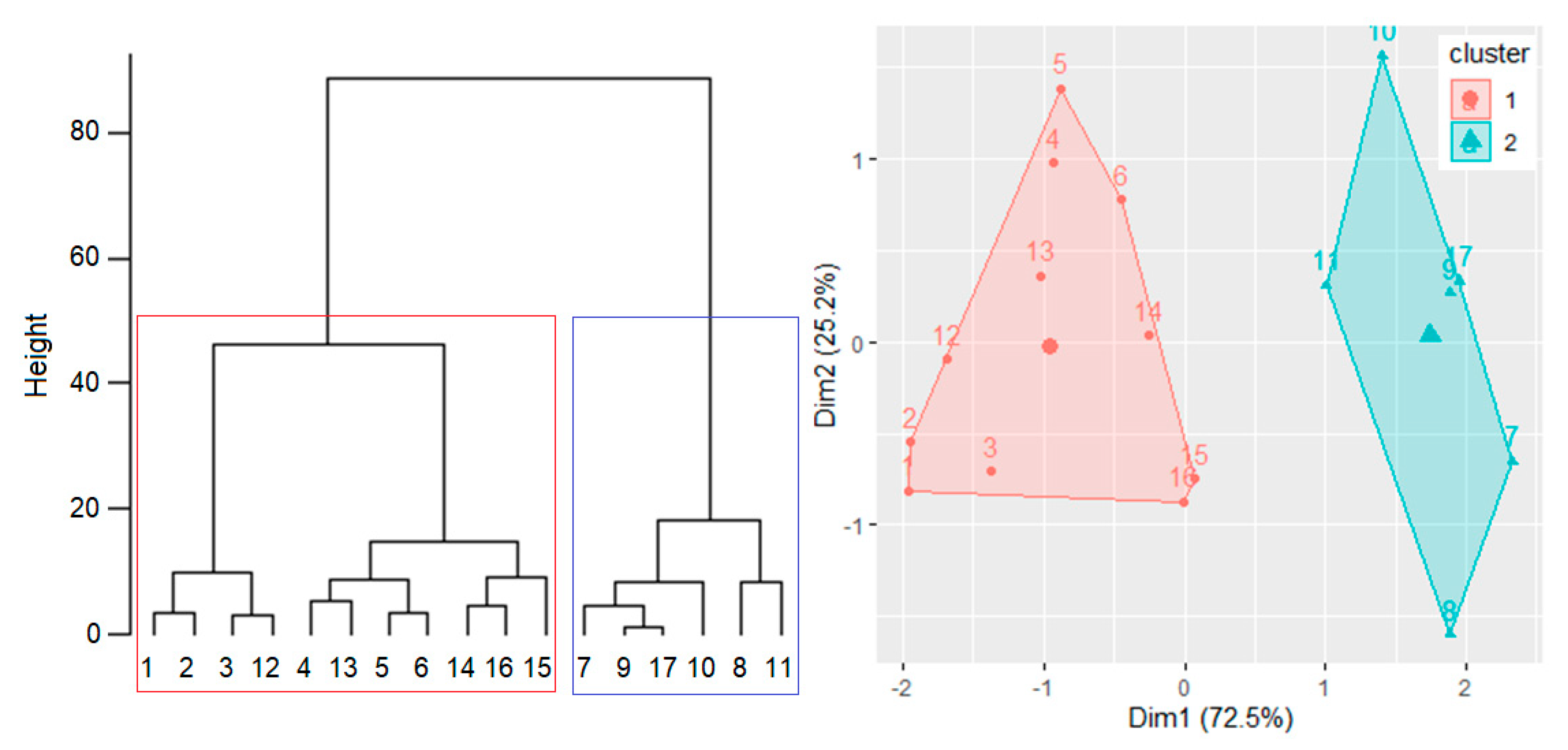
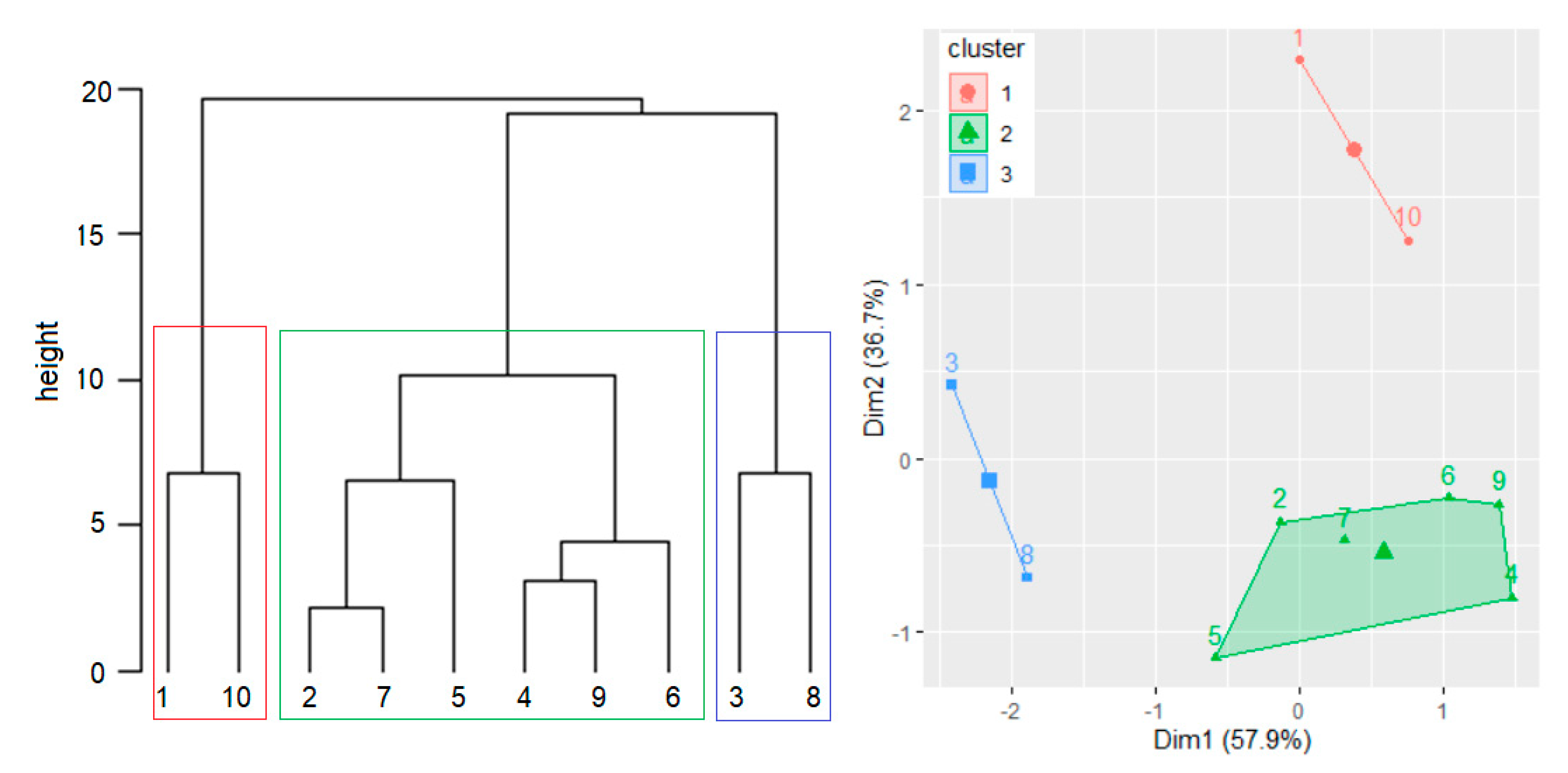
3.3. Clustering Data Series
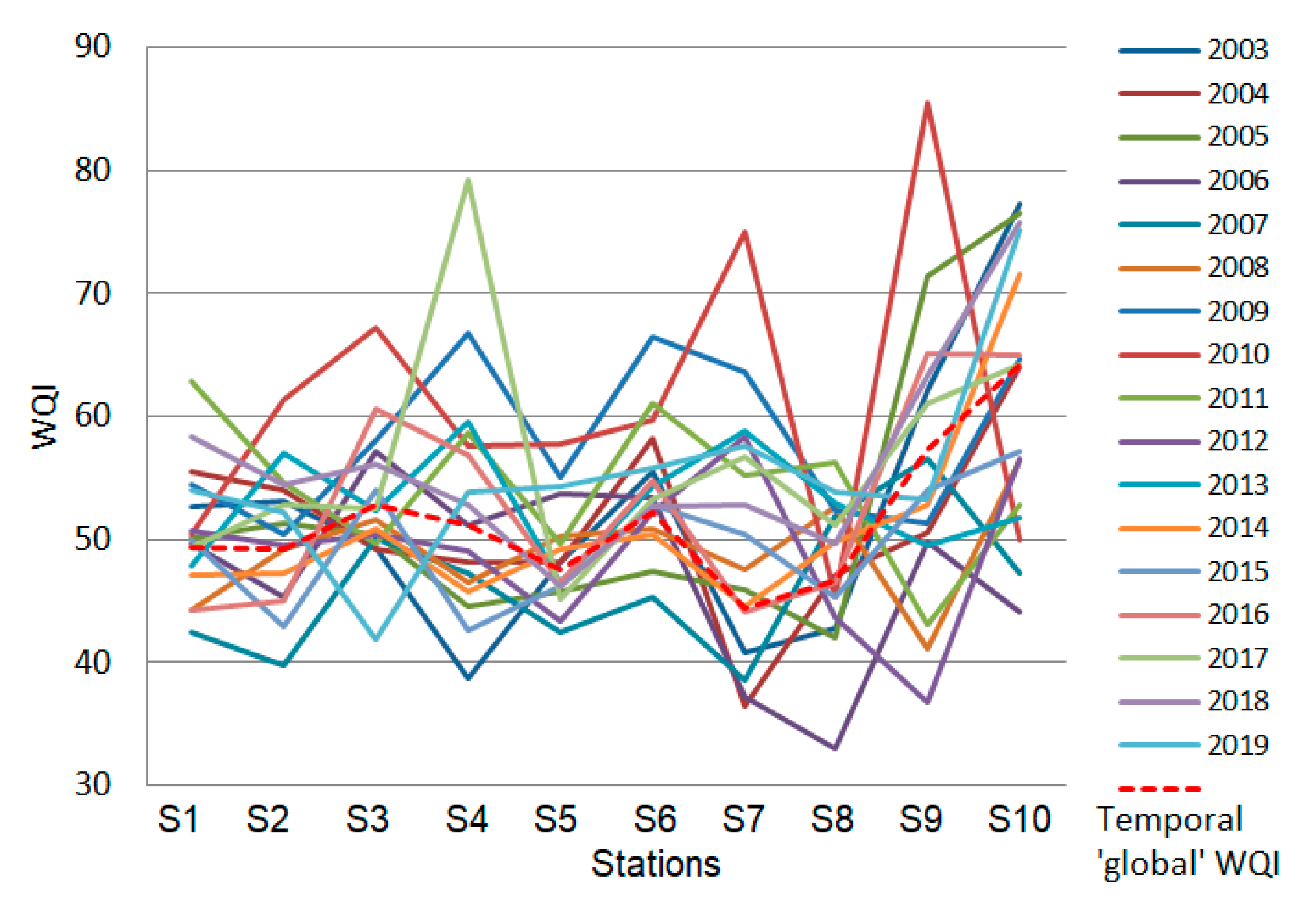
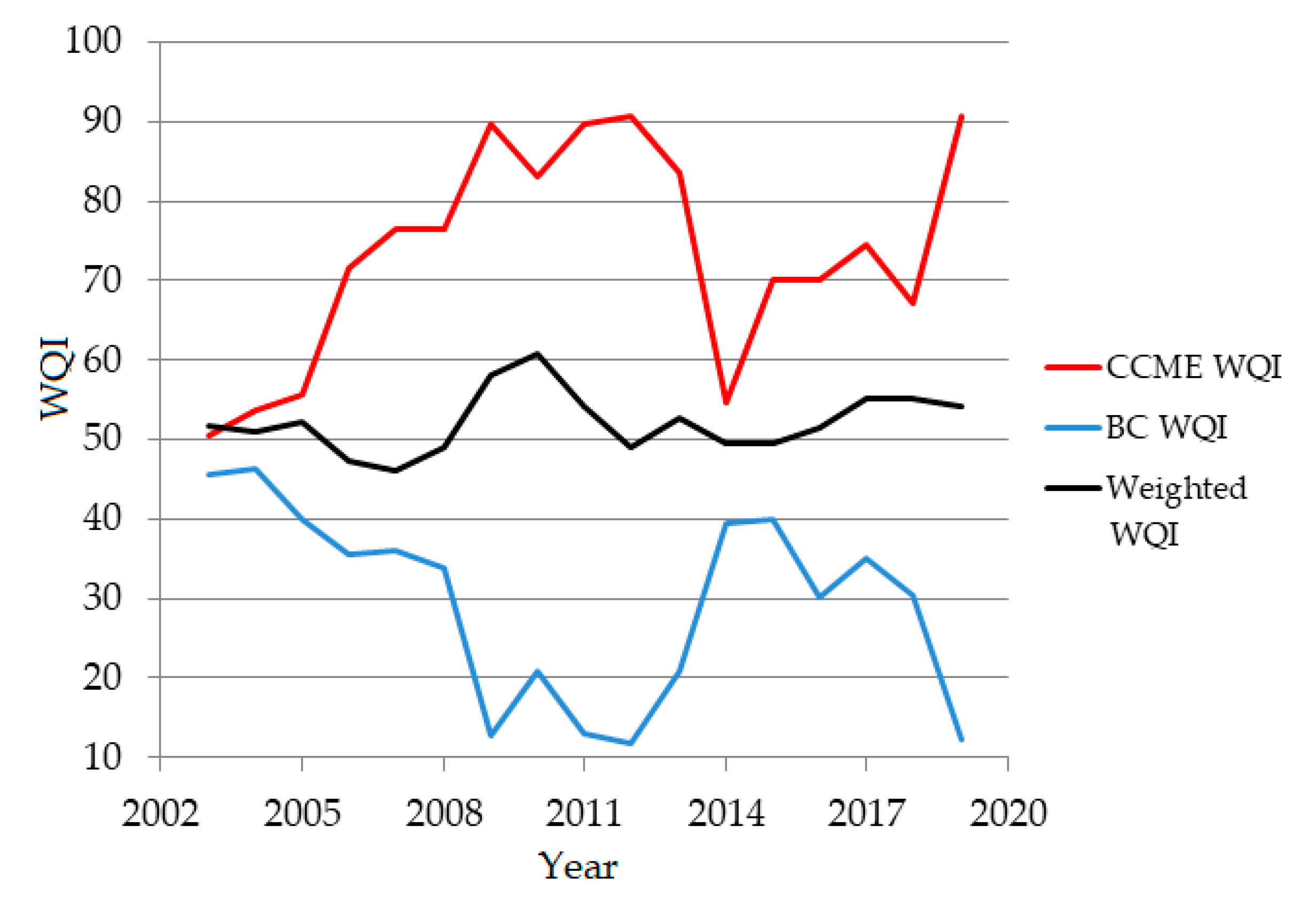
3.4. Determination of the Regional Series and Temporal ‘Global’ Series
3.5. Discussions of the Present Results Compared with Previous Research
4. Conclusions
Author Contributions
Funding
Institutional Review Board Statement
Informed Consent Statement
Data Availability Statement
Conflicts of Interest
References
- Singh, A.; Sharam, R.K.; Agrawal, M.; Marshall, F.M. Health risk assessment of heavy metals via dietary intake of foodstuffs from the wastewater irrigated site of a dry tropical area of India. Food Chem. Toxicol. 2010, 48, 611–619. [Google Scholar] [CrossRef]
- U.S. Environmental Protection Agency (EPA). Ecological Risk Models and Tools. 2021. Available online: https://www.epa.gov/risk/ecological-risk-models-and-tools (accessed on 20 September 2021).
- Avigliano, E.; Schenone, N.F. Human health risk assessment and environmental distribution of trace elements, glyphosate, fecal coliform and total coliform in Atlantic Rainforest mountain rivers (South America). Microchem. J. 2015, 122, 149–158. [Google Scholar] [CrossRef]
- Mekuria, D.M.; Kassegne, A.B.; Asfaw, S.L. Assessing pollution profiles along Little Akaki River receiving municipal and industrial wastewaters, Central Ethiopia: Implications for environmental and public health safety. Heliyon 2021, 7, e07526. [Google Scholar] [CrossRef]
- Bărbulescu, A.; Maftei, C.; Dumitriu, C.S. The modelling of the climateric process that participates at the sizing of an irrigation system. Bull. Appl. Comput. Math. 2002, 2048, 11–20. [Google Scholar]
- Nambatingar, N.; Clement, Y.; Merle, A.; New Mahamat, T.; Lanteri, P. Heavy metal pollution of Chari river water during the crossing of N’Djamena (Chad). Toxics 2017, 5, 26. [Google Scholar] [CrossRef]
- Zhou, T.; Wu, J.; Peng, S. Assessing the effects of landscape pattern on river water quality at multiple scales: A case study of the Dongjiang River watershed, China. Ecol. Indic. 2012, 23, 166–175. [Google Scholar] [CrossRef]
- Campanale, C.; Dierkes, G.; Massarelli, C.; Bagnuolo, G.; Uricchio, V.F. A relevant screening of organic contaminants present on freshwater and pre-production microplastics. Toxics 2020, 8, 100. [Google Scholar] [CrossRef] [PubMed]
- Al-Taani, A.; Nazzal, Y.; Howari, F.; Iqbal, J.; Bou-Orm, N.; Xavier, C.M.; Bărbulescu, A.; Sharma, M.; Dumitriu, C.S. Contamination assessment of heavy metals in soil, Liwa area, UAE. Toxics 2021, 9, 53. [Google Scholar] [CrossRef] [PubMed]
- Mihăilescu, M.; Negrea, A.; Ciopec, M.; Negrea, P.; Duțeanu, N.; Grozav, I.; Svera, P.; Vancea, C.; Bărbulescu, A.; Dumitriu, C.S. Full factorial design for gold recovery from industrial solutions. Toxics 2021, 9, 111. [Google Scholar] [CrossRef]
- Nazzal, Y.H.; Bărbulescu, A.; Howari, F.; Al-Taani, A.A.; Iqbal, J.; Xavier, C.M.; Sharma, M. Dumitriu, C.Ș. Assessment of metals concentrations in soils of Abu Dhabi Emirate using pollution indices and multivariate statistics. Toxics 2021, 9, 95. [Google Scholar] [CrossRef] [PubMed]
- Pisciotta, J.M.; Rath, D.F.; Stanek, P.A.; Flanery, D.M.; Harwood, V.J. Marine bacteria cause false-positive results in the colilert-18 rapid identification test for escherichia coli in florida waters. Appl. Environ. Microbiol. 2002, 68, 539–544. [Google Scholar] [CrossRef] [PubMed] [Green Version]
- Seo, M.; Lee, H.; Kim, Y. Relationship between coliform bacteria and water quality factors at weir stations in the Nakdong River, South Korea. Water 2019, 11, 1171. [Google Scholar] [CrossRef] [Green Version]
- Aonofriesei, F.; Bărbulescu, A.; Dumitriu, C.-S. Statistical analysis of morphological parameters of microbial aggregates in the activated sludge from a wastewater treatment plant for improving its performances. Rom. J. Phys. 2021, 66, 809. [Google Scholar]
- Vadde, K.K.; Jianjun, W.; Long, C.; Tianma, Y.; Alan, J.; Raju, S. Assessment of water quality and identification of pollution rick locations in Tiaoxi River (Taihu watershed), China. Water 2017, 10, 183. [Google Scholar] [CrossRef] [Green Version]
- Xu, H.; Paerl, H.W.; Qin, B.; Zhu, G.; Gaoa, G. Nitrogen and phosphorus inputs control phytoplankton growth in eutrophic Lake Taihu, China. Limnol. Oceanogr. 2010, 55, 420–432. [Google Scholar] [CrossRef] [Green Version]
- Gupta, S.; Gupta, S.K. A critical review on water quality index tool: Genesis, evolution and future directions. Ecol. Inform. 2021, 63, 101299. [Google Scholar] [CrossRef]
- Bărbulescu, A. Assessing groundwater vulnerability: DRASTIC and DRASTIC-like methods: A review. Water 2020, 12, 1356. [Google Scholar] [CrossRef]
- Bărbulescu, A.; Dumitriu, C.Ș. Assessing the water quality by statistical methods. Water 2021, 13, 1026. [Google Scholar] [CrossRef]
- Bărbulescu, A.; Barbeş, L. Assessing the water quality of the Danube River (at Chiciu, Romania) by statistical methods. Environ. Earth Sci. 2020, 79, 122. [Google Scholar] [CrossRef]
- Razmkhah, H.; Abrishamchi, A.; Torkian, A. Evaluation of spatial and temporal variation in water quality by pattern recognition techniques: A case study on jajrood river (Tehran, Iran). J. Environ. Manag. 2010, 91, 852–860. [Google Scholar] [CrossRef]
- Ogwueleka, T.C. Use of multivariate statistical techniques for the evaluation of temporal and spatial variations in water quality of the Kaduna River, Nigeria. Environ. Monit. Assess. 2015, 187, 137. [Google Scholar] [CrossRef]
- Sheikhy Narany, T.; Ramli, M.F.; Aris, A.Z.; Sulaiman, W.N.; Fakharian, K. Spatiotemporal variation of groundwater quality using integrated multivariate statistical and geostatistical approaches in Amol-Babol Plain. Iran. Environ. Monit. Assess. 2014, 186, 5797–5815. [Google Scholar] [CrossRef] [PubMed]
- Sharma, A.; Bora, C.R.; Shukla, V. Evaluation of seasonal changes in physico-chemical and bacteriological characteristics of water from the Narmada River (India) using multivariate analysis. Nat. Resour. Res. 2013, 22, 283–296. [Google Scholar] [CrossRef]
- Bărbulescu, A.; Postolache, F.; Dumitriu, C.Ș. Estimating the precipitation amount at regional scale using a new tool, Climate Analyzer. Hidrology 2021, 8, 125. [Google Scholar] [CrossRef]
- Dragomir, F.L. Modeling and Simulation of the Systems and Processes; Editura Universității Naționale de Apărare Carol I: București, Romania, 2017. (In Romanian) [Google Scholar]
- Dragomir, F.L. Decision Theory—Theoretical Notions; Editura Universității Naționale de Apărare Carol I: București, Romania, 2017. (In Romanian) [Google Scholar]
- Dragomir, F.L. Operational Research; Editura Universității Naționale de Apărare Carol I: București, Romania, 2017. (In Romanian) [Google Scholar]
- Tiyasha, S.; Tung, T.M.; Yaseen, Z.M. A survey on river water quality modelling using artificial intelligence models: 2000–2020. J. Hydrol. 2020, 585, 124670. [Google Scholar] [CrossRef]
- Jiang, Y.; Nan, Z.; Yang, S. Risk assessment of water quality using Monte Carlo simulation and artificial neural network method. J. Environ. Manag. 2013, 122, 130–136. [Google Scholar] [CrossRef]
- Divya, A.H.; Soloman, P.A. Assessment of river water quality indices based on various fuzzy models and arithmetic indexing method. IOP Conf. Ser. Mater. Sci. Eng. 2021, 1114, 012092. [Google Scholar] [CrossRef]
- Landwehr, J.M. A statistic view of a class of water quality indices. Water Resour. Res. 1979, 15, 460–468. [Google Scholar] [CrossRef]
- House, M.A.; Newsome, D.H. Water quality indices for the management of surface water quality. Water Sci. Technol. 1989, 21, 1137–1148. [Google Scholar] [CrossRef]
- Horton, R.K. An index number system for rating water quality. J. Wat. Pollut. Con. Fed. 1965, 37, 300–305. [Google Scholar]
- Uddin, M.G.; Nash, S.; Olbert, A.I. A review of water quality index models and their use for assessing surface water quality. Ecol. Indic. 2021, 122, 107218. [Google Scholar] [CrossRef]
- Bascaron, M. Establishment of a methodology for the determination of water quality. Bull. Inform. Medio Amb. 1979, 9, 30–51. [Google Scholar]
- CCME, Canadian Water Quality Index 1.0. Technical Report and User’s Manual Gatineau, QC: Canadian Council of Minister of the Environment, Canadian Environmental Quality Guidelines, Water Quality Index Technical Subcommittee. 2021. Available online: http://ceqg-rcqe.ccme.ca/download/en/138 (accessed on 15 August 2020).
- Dinius, S.H. Design of an Index of Water Quality. J. Am. Water Resour. Assoc. 1987, 23, 833–843. [Google Scholar] [CrossRef]
- Cude, C.G. Oregon water quality index: A tool for evaluating water quality management effectiveness. J. Am. Water Resour. Assoc. 2001, 37, 125–137. [Google Scholar] [CrossRef]
- Sutadian, A.D.; Muttil, N.; Yilmaz, A.G.; Perera, B.J.C. Development of a water quality index for rivers in West Java Province, Indonesia. Ecol. Indic. 2018, 85, 966–982. [Google Scholar] [CrossRef]
- Gupta, A.K.; Gupta, S.K.; Patil, R.S. A comparison of water quality indices for coastal water. J. Environ. Sci. Health Part A 2003, 38, 2711–2725. [Google Scholar] [CrossRef]
- Almeida, C.; Gonzalez, S.O.; Mallea, M.; Gonzalez, P. A recreational water quality index using chemical, physical and microbiological parameters. Environ. Sci. Pollut. Res. 2012, 19, 3400–3411. [Google Scholar] [CrossRef]
- Dojlido, J.A.N.; Raniszewski, J.; Woyciechowska, J. Water quality index applied to rivers in the Vistula River basin in Poland. Environ. Monit. Assess. 1994, 33, 33–42. [Google Scholar] [CrossRef]
- Liou, S.-M.; Lo, S.-L.; Wang, S.-H. A Generalized Water Quality Index for Taiwan. Environ. Monit. Assess. 2004, 96, 35–52. [Google Scholar] [CrossRef]
- MacDonald, D.D.; Berger, T.; Wood, K.; Brown, J.; Johnsen, T.; Haines, M.L.; Brydges, K.; MacDonald, M.J.; Smith, S.L.; Shaw, D.P. A Compendium of Environmental Quality Benchmarks. Available online: https://www.lm.doe.gov/cercla/documents/rockyflats_docs/SW/SW-A-005694.pdf (accessed on 2 November 2021).
- Rocchini, R.; Swain., L.G. The British Columbia Water Quality Index; Water Quality Branch, Environmental Protection Department British Columbia Ministry of Environment, Lands and Parks: Victoria, BC, Canada, 1995; p. 13. [Google Scholar]
- Wright, C.R.; Saffran, K.A.; Anderson, A.-M.; Neilson, R.D.; MacAlpine, N.D.; Cooke, S.E. A Water Quality Index for Agricultural Streams in Alberta: The Alberta Agricultural Water Quality Index (AAWQI); Prepared for the Alberta Environmentally Sustainable Agriculture Program (AESA). Alberta Agriculture, Food and Rural Development: Edmonton, AB, Canada, 1999; p. 35. [Google Scholar]
- Granata, F.; Papirio, S.; Esposito, G.; Gargano, R.; de Marinis, G. Machine Learning Algorithms for the Forecasting of Wastewater Quality Indicators. Water 2017, 9, 105. [Google Scholar] [CrossRef] [Green Version]
- Oladipo, J.O.; Akinwumiju, A.S.; Aboyeji, O.S.; Adelodun, A.A. Comparison between fuzzy logic and water quality index methods: A case of water quality assessment in Ikare community, Southwestern Nigeria. Environ. Chall. 2021, 3, 100038. [Google Scholar] [CrossRef]
- Shah, M.I.; Alaloul, W.S.; Alqahtani, A.; Aldrees, A.; Musarat, M.A.; Javed, M.F. Predictive Modeling Approach for Surface Water Quality: Development and Comparison of Machine Learning Models. Sustainability 2021, 13, 7515. [Google Scholar] [CrossRef]
- Bărbulescu, A.; Nazzal, Y.; Howari, F. Assessing the groundwater quality in the Liwa area, the United Arab Emirates. Water 2020, 12, 2816. [Google Scholar] [CrossRef]
- Du, X.; Feng, J.; Fang, M.; Ye, X. Sources, Influencing Factors, and Pollution Process of Inorganic Nitrogen in Shallow Groundwater of a Typical Agricultural Area in Northeast China. Water 2020, 12, 3292. [Google Scholar] [CrossRef]
- Mamun, M.; Kim, J.Y.; An, K.-G. Multivariate Statistical Analysis of Water Quality and Trophic State in an Artificial Dam Reservoir. Water 2021, 13, 186. [Google Scholar] [CrossRef]
- Al-Taani, A.A.; Rashdan, M.; Nazzal, Y.; Howari, F.; Iqbal, J.; Al-Rawabdeh, A.; Al Bsoul, A.; Khashashneh, S. Evaluation of the Gulf of Aqaba Coastal Water, Jordan. Water 2020, 12, 2125. [Google Scholar] [CrossRef]
- Yu, Y.; Song, X.; Zhang, Y.; Zheng, F. Assessment of Water Quality Using Chemometrics and Multivariate Statistics: A Case Study in Chaobai River Replenished by Reclaimed Water, North China. Water 2020, 12, 2551. [Google Scholar] [CrossRef]
- Cui, L.; Wang, X.; Li, J.; Gao, X.; Zhang, J.; Liu, Z. Ecological and health risk assessments and water quality criteria of heavy metals in the Haihe River. Environ. Poll. 2021, 290, 117971. [Google Scholar] [CrossRef] [PubMed]
- Reitter, C.; Petzoldt, H.; Korth, H.; Schwab, F.; Stange, C.; Hambsch, B.; Tiehm, A.; Lagkouvardos, I.; Gescher, J.; Hügler, M. Seasonal dynamics in the number and composition of coliform bacteria in drinking water reservoirs. Sci. Total. Environ. 2021, 787, 147539. [Google Scholar] [CrossRef]
- Rising Problems and Solutions to Water Pollution in India. Available online: https://www.borgenmagazine.com/water-in-india/ (accessed on 25 July 2021).
- Water Pollution is Killing Millions of Indians. Here’s How Technology and Reliable Data Can Change That. Available online: https://www.weforum.org/agenda/2019/10/water-pollution-in-india-data-tech-solution/ (accessed on 25 July 2021).
- Pollution Assessment. River Ganga. Available online: https://cpcb.nic.in/wqm/pollution-assessment-ganga-2013.pdf (accessed on 25 July 2021).
- Avvannavar, S.M.; Shrihari, S. Evaluation of water quality index for drinking purposes for river Netravathi, Mangalore, South India. Environ. Monit. Assess. 2008, 143, 279–290. [Google Scholar] [CrossRef] [PubMed]
- Bhargava, D.S. Use of a water quality index for river classification and zoning of the Ganga River. Environ. Poll. 1983, B6, 51–67. [Google Scholar] [CrossRef]
- Rakhecha, P.R. Water environment pollution with its impact on human diseases in India. Int. J. Hydrol. 2020, 4, 152–158. [Google Scholar] [CrossRef]
- Bora, M.; Goswami, D.C. Water quality assessment in terms of water quality index (WQI): Case study of the Kolong River, Assam, India. Appl. Water Sci. 2017, 7, 3125–3135. [Google Scholar] [CrossRef] [Green Version]
- Bărbulescu, A.; Barbeş, L.; Dumitriu, C.Ş. Statistical assessment of the water quality using water quality indicators. A case study from India. In Water Safety and Security—Threat Detection and Mitigation, Advanced Sciences and Technologies for Security Applications; Vaseashta, A.K., Maftei, C., Eds.; Springer International Publishing AG: Cham, Switzerland, 2021; pp. 599–613. [Google Scholar]
- Bărbulescu, A.; Dani, A. Statistical analysis and classification of the water parameters of Beas River (India). Rom. Rep. Phys. 2019, 71, 716. [Google Scholar]
- Chakrabarty, S.; Sarma, H.P. A statistical approach to multivariate analysis of drinking water quality in Kamrup district, Assam, India. Arch. Appl. Sci. Res. 2011, 3, 258–264. [Google Scholar]
- Dimri, D.; Daverey, A.; Kumar, A.; Sharma, A. Monitoring water quality of River Ganga using multivariate techniques and WQI (Water Quality Index) in Western Himalayan region of Uttarakhand, India. Environ. Nanotechnol. Monit. Manag. 2021, 15, 100375. [Google Scholar]
- Singh, K.P.; Malik, A.; Sinha, S. Water quality assessment and apportionment of pollution sources of Gomti River (India) using, multivariate statistical techniques—A case study. Anal. Chem. Acta 2005, 538, 355–374. [Google Scholar] [CrossRef]
- Bhuyan, M.; Bakar, M.; Sharif, A.; Hasan, M.; Islam, M. Water quality assessment using water quality indicators and multivariate analyses of the Old Brahmaputra River. Pollution 2018, 4, 481–493. [Google Scholar]
- Gangwar, S. Water quality monitoring in India: A review. Int. J. Inform. Comput. Technol. 2013, 3, 851–856. [Google Scholar]
- Immerzeel, W. Historical trends and future predictions of climate variability in the Brahmaputra basin. Int. J. Climatol. 2008, 28, 243–254. [Google Scholar] [CrossRef]
- Datta, B.; Singh, V.P. Hydrology. In The Brahmaputra Basin Water Resources; Singh, V., Sharma, N., Ojha, C.S.P., Eds.; Kluwer Academic Publishers: New York, NY, USA, 2004; pp. 139–195. [Google Scholar]
- Purkait, B. Hydrometeorology. In The Brahmaputra Basin Water Resources; Singh, V., Sharma, N., Ojha, C.S.P., Eds.; Kluwer Academic Publishers: New York, NY, USA, 2004; Volume 47, pp. 24–34. [Google Scholar]
- Sarma, J.N. An overview of the Brahmaputra river system. In The Brahmaputra Basin Water Resources; Singh, V., Sharma, N., Ojha, C.S.P., Eds.; Kluwer Academic Publishers: New York, NY, USA, 2004; Volume 47, pp. 72–87. [Google Scholar]
- Mahanta, C.; Zaman, A.M.; Newaz, A.M.S.; Rahman, S.M.M.; MAzumdar, T.K.; Choudhury, R.; Borah, P.J.; Saikia, L. Physical assessment of the Brahmaputra River. In Ecosystems for Life: A Bangladesh-India Initiative; Prokashony, J., Ed.; International Union for Conservation of Nature: Dhaka, Bangladesh, 2014; p. 74. Available online: https://portals.iucn.org/library/node/45928 (accessed on 20 September 2021).
- Amarasinghe, U.A.; Sharma, B.R.; Aloysius, N.; Scott, C.; Smakhtin, V.; de Fraiture, C.; Shukla, A.K. Spatial Variation in Water Supply and Demand Across the River Basins of India; Research Report 83. International Water Management Institute: Colombo, Sri Lanka, 2004. Available online: https://www.iwmi.cgiar.org/publications/iwmi-research-reports/iwmi-research-report-83/ (accessed on 20 September 2021).
- ENVIS Centre on Control of Pollution Water, Air and Noise, Water Quality Database. Available online: http://www.cpcbenvis.nic.in/water_quality_data.html# (accessed on 15 September 2021).
- Kendall, M.G. Rank Correlation Methods, 4th ed.; Charles Griffin: London, UK, 1975. [Google Scholar]
- Sen, P.K. Estimates of the regression coefficient based on Kendall’s tau. J. Am. Stat. Assoc. 1968, 63, 1379–1389. [Google Scholar] [CrossRef]
- Corder, G.W.; Foreman, D.I. Nonparametric Statistics for Non-Statisticians; John Wiley & Sons: Hoboken, NJ, USA, 2009. [Google Scholar]
- Cleveland, W.S.; Grosse, E.; Shyu, W.M. Local regression models. In Statistical Models in S; Chambers, J.M., Hastie, T.J., Eds.; Wadsworth & Brooks/Cole: Pacific Grove, CA, USA, 1992. [Google Scholar]
- Canadian Council of Ministers of the Environment. CCME WATER QUALITY INDEX 1.0 User’s Manual 2017 Update; Environment and Climate Change Canada Guidelines and Standards Division: Gatineau, QC, Canada, 2017. [Google Scholar]
- Zandbergen, P.A.; Hall, K.J. Analysis of British Columbia Water Quality Index for Warweshed Managers: A Case Study of Two Small Watersheds. Water Qual. Res. J. Can. 1998, 33, 519–549. [Google Scholar] [CrossRef]
- Everitt, B.S.; Landau, S.; Leese, M.; Stahl, D. Cluster Analysis; John Wiley & Sons, Ltd.: Hoboken, NJ, USA, 2011. [Google Scholar]
- Charrad, M.; Ghazzali, G.N.; Boiteau, V.; Nicknafs, A. NbClust: An R Package for Determining the Relevant Number of Clusters in a Data Set. J. Stat. Softw. 2014, 61, 1–36. [Google Scholar] [CrossRef] [Green Version]
- Muyen, Z.; Rashedujjaman, M.; Rahman, M.S. Assessment of water quality index: A case study in Old Brahmaputra river of Mymensingh District in Bangladesh. Progress. Agric. 2016, 27, 355–361. [Google Scholar] [CrossRef] [Green Version]
- Kotoky, P.; Sharma, B. Assessment of Water Quality Index of the Brahmaputra River of Guwahati City of Kamrup, District of Assam, India. Int. J. Eng. Res. Technol. 2017, 6, 536–540. [Google Scholar]
- Mech, A.; Hazarika, P. A Study on the Impact of Industrial Effluents on Local Ecosystem and Willingness to pay for its Restoration. Amity J. Ec. 2018, 3, 61–74. [Google Scholar]
- Tsering, T.; Sillanpää, M.; Sillanpää, M.; Viitala, M.; Reinikainen, S.-P. Microplastics pollution in the Brahmaputra River and the Indus River of the Indian Himalaya. Sci. Total Environ. 2021, 789, 147968. [Google Scholar] [CrossRef] [PubMed]
- Reports on Water Quality Scenario of Rivers. Government of India, Ministry of Jal Shakti, Department of Water Resources, River Development & Ganga Rejuvenation, CWC/2021/19(V-IV). 2021. Available online: http://www.cwc.gov.in/sites/default/files/volume-4.pdf (accessed on 22 October 2021).
- Fresh Water under Threat. South Asia. United Nations Environment Programme. 2008. Available online: https://wedocs.unep.org/bitstream/handle/20.500.11822/7715/-FreshWater%20under%20threat%20South%20Asia-2009846.pdf?sequence=3&isAllowed=y (accessed on 22 October 2021).


| Sen Slope | S1 | S2 | S3 | S4 | S5 | S6 | S7 | S8 | S9 | S10 |
|---|---|---|---|---|---|---|---|---|---|---|
| Temperature | 0.150 | −0.221 | - | - | - | −0.100 | - | - | 0.293 | 0.200 |
| pH | 0.047 | - | - | −0.027 | - | - | - | - | - | - |
| EC | −10.500 | −9.076 | - | - | −3.632 | −4.903 | - | −4.819 | −12.667 | - |
| DO | - | - | - | - | - | - | −0.100 | −0.044 | - | - |
| BOD | - | - | - | 0.071 | - | - | - | - | - | - |
| Nitrate and Nitrite | 0.084 | 0.028 | 0.055 | 0.052 | 0.041 | 0.020 | 0.021 | 0.044 | 0.049 | 0.046 |
| FC | −144.792 | - | - | - | - | - | - | −0.833 | - | - |
| TC | - | - | - | - | - | - | - | - | - | - |
| Year | 2003 | 2004 | 2005 | 2006 | 2007 | 2008 | 2009 | 2010 | 2011 |
|---|---|---|---|---|---|---|---|---|---|
| Temperature | - | - | - | - | - | 0.714 | 0.275 | - | 0.456 |
| pH | - | - | - | - | - | - | - | - | - |
| EC | - | - | - | −10.500 | - | - | - | 4.500 | - |
| DO | - | - | - | - | - | - | - | - | - |
| BOD | - | - | - | - | - | - | - | - | - |
| Nitrate and Nitrite | - | - | - | - | - | - | - | - | - |
| FC | - | - | - | - | - | - | - | - | - |
| TC | - | - | - | - | - | - | - | - | - |
| Year | 2012 | 2013 | 2014 | 2015 | 2016 | 2017 | 2018 | 2019 | |
| Temperature | 0.600 | 0.500 | 0.656 | - | 0.500 | 0.833 | 0.667 | 1.000 | |
| pH | - | - | - | - | - | - | - | - | |
| EC | - | - | - | - | - | - | - | - | |
| DO | - | - | - | - | - | - | - | - | |
| BOD | - | - | - | - | - | - | - | - | |
| Nitrate+Nitrite | - | - | - | - | - | - | - | - | |
| FC | - | - | - | - | - | - | 172.000 | - | |
| TC | - | - | - | - | - | - | - | - |
| Station | CCME WQI | BC WQI | Weighted WQI | |||
|---|---|---|---|---|---|---|
| Value | Class | Value | Class | Value | Class | |
| S1 | 68.56 | Fair | 41.07 | Fair | 66.42 | Poor |
| S2 | 65.33 | Fair | 41.93 | Fair | 50.61 | Good/Poor |
| S3 | 72.54 | Fair | 34.68 | Fair | 53.03 | Poor |
| S4 | 55.59 | Marginal | 43.57 | Fair/Borderline | 52.89 | Poor |
| S5 | 60.81 | Marginal | 37.63 | Fair | 48.74 | Good |
| S6 | 59.74 | Marginal | 43.53 | Fair/Borderline | 54.35 | Poor |
| S7 | 63.43 | Marginal | 42.92 | Fair | 50.81 | Good/Poor |
| S8 | 68.12 | Fair | 35.71 | Fair | 48.03 | Good |
| S9 | 56.89 | Marginal | 43.31 | Fair/Borderline | 55.72 | Poor |
| S10 | 64.02 | Marginal | 43.07 | Fair/Borderline | 61.78 | Poor |
| Station | CCME WQI | BC WQI | Weighted | |||
|---|---|---|---|---|---|---|
| Value | Class | Value | Class | Value | Class | |
| 2003 | 50.60 | Marginal | 45.46 | Bordeline | 51.66 | Poor |
| 2004 | 53.74 | Marginal | 46.21 | Bordeline | 50.85 | Good/Poor |
| 2005 | 55.67 | Marginal | 40.03 | Fair | 52.23 | Poor |
| 2006 | 71.58 | Fair | 35.43 | Fair | 47.34 | Good |
| 2007 | 76.37 | Fair | 36.00 | Fair | 46.15 | Good |
| 2008 | 76.37 | Fair | 33.77 | Fair | 48.91 | Good |
| 2009 | 89.74 | Good | 12.84 | Good | 58.19 | Poor |
| 2010 | 83.13 | Good | 20.87 | Fair | 60.84 | Poor |
| 2011 | 89.74 | Good | 12.98 | Good | 54.25 | Poor |
| 2012 | 90.73 | Good | 11.81 | Good | 48.91 | Good |
| 2013 | 83.49 | Good | 20.76 | Fair | 52.72 | Poor |
| 2014 | 54.67 | Marginal | 39.43 | Fair | 49.53 | Poor |
| 2015 | 70.09 | Fair | 39.96 | Fair | 49.46 | Good |
| 2016 | 70.09 | Fair | 30.25 | Fair | 51.54 | Poor |
| 2017 | 74.40 | Fair | 34.99 | Fair | 55.09 | Poor |
| 2018 | 67.06 | Fair | 30.27 | Fair | 55.06 | Poor |
| 2019 | 90.70 | Good | 12.33 | Good | 54.13 | Poor |
| S1 | S2 | S3 | S4 | S5 | S6 | S7 | S8 | S9 | S10 | |
|---|---|---|---|---|---|---|---|---|---|---|
| MAE | 4.72 | 3.42 | 3.92 | 5.16 | 4.47 | 4.05 | 5.51 | 6.05 | 8.50 | 12.44 |
| RMSE | 6.10 | 4.02 | 5.04 | 6.96 | 5.34 | 4.64 | 6.49 | 7.66 | 9.94 | 14.61 |
| MAPE | 0.33 | 0.38 | 0.05 | 1.67 | 0.19 | 0.61 | 1.30 | 0.95 | 1.18 | 2.10 |
| 2003 | 2004 | 2005 | 2006 | 2007 | 2008 | 2009 | 2010 | 2011 | ||
|---|---|---|---|---|---|---|---|---|---|---|
| MAE | 5.25 | 3.94 | 5.06 | 6.45 | 6.39 | 4.80 | 8.02 | 12.60 | 8.67 | |
| RMSE | 6.52 | 4.78 | 6.69 | 8.81 | 7.64 | 6.55 | 9.97 | 15.77 | 9.51 | |
| MAPE | 0.63 | 1.11 | 0.15 | 0.04 | 1.64 | 1.15 | 0.92 | 0.20 | 2.14 | |
| 2012 | 2013 | 2014 | 2015 | 2016 | 2017 | 2018 | 2019 | |||
| MAE | 5.56 | 6.22 | 3.02 | 3.64 | 3.58 | 5.57 | 5.00 | 6.73 | ||
| RMSE | 8.46 | 7.77 | 3.63 | 4.63 | 4.56 | 9.94 | 6.10 | 7.62 | ||
| MAPE | 0.27 | 0.32 | 0.47 | 0.12 | 1.18 | 0.00 | 1.54 | 0.86 | ||
Publisher’s Note: MDPI stays neutral with regard to jurisdictional claims in published maps and institutional affiliations. |
© 2021 by the authors. Licensee MDPI, Basel, Switzerland. This article is an open access article distributed under the terms and conditions of the Creative Commons Attribution (CC BY) license (https://creativecommons.org/licenses/by/4.0/).
Share and Cite
Barbulescu, A.; Barbes, L.; Dumitriu, C.S. Assessing the Water Pollution of the Brahmaputra River Using Water Quality Indexes. Toxics 2021, 9, 297. https://doi.org/10.3390/toxics9110297
Barbulescu A, Barbes L, Dumitriu CS. Assessing the Water Pollution of the Brahmaputra River Using Water Quality Indexes. Toxics. 2021; 9(11):297. https://doi.org/10.3390/toxics9110297
Chicago/Turabian StyleBarbulescu, Alina, Lucica Barbes, and Cristian Stefan Dumitriu. 2021. "Assessing the Water Pollution of the Brahmaputra River Using Water Quality Indexes" Toxics 9, no. 11: 297. https://doi.org/10.3390/toxics9110297
APA StyleBarbulescu, A., Barbes, L., & Dumitriu, C. S. (2021). Assessing the Water Pollution of the Brahmaputra River Using Water Quality Indexes. Toxics, 9(11), 297. https://doi.org/10.3390/toxics9110297