Abstract
Inverse least squares numerical optimization, 3D/4D interior optimization, and 3D/4D graphical optimization software and algorithm programming have been presented in a series of previous articles on the applications of the BCS theory of superconductivity and TC dual/multiobjective optimizations. This study deals with the comparison/validation of the optimization results using several different methods, namely, classical inverse least squares (ILS), genetic algorithms (GA), 3D/4D interior optimization, and 2D/3D/4D graphical optimization techniques. The results comprise Tikhonov regularization algorithms and mathematical methods for all the research subjects. The findings of the mathematical programming for optimizing type I chrome isotope superconductors are validated with the genetic algorithms and compared to previous results of 3D/4D interior optimization. Additional rulings present a hypothesis of the new ‘molecular effect’ model/algorithm intended to be proven for Hg-cuprate-type high-temperature superconductors. In molecular effect optimization, inverse least squares and inverse least squares polynomial methods are applied with acceptable numerical and 2D graphical optimization solutions. For the BCS isotope effect and molecular effect, linearization logarithmic transformations for model formula software are implemented in specific programs. The solutions show accuracy with low programming residuals and confirm these findings. The results comprise two strands, the modeling for the isotope effect and molecular effect hypotheses and the development of genetic algorithms and inverse least squares-improved programming methods. Electronic physics applications in superconductors and high-temperature superconductors emerged from the rulings. Extrapolated applications for new modeling for the theory of superconductivity emerged from the numerical and image data obtained.
1. Introduction
A superconductor can be defined as any material type whose electrical resistance is approximately null under specific thermodynamic and electromagnetic conditions. The essential thermodynamic conditions needed to reach the superconductivity state are given by a critical temperature TC, beyond which, toward lower temperatures, a superconductivity effect takes place and interactions with magnetic fields constitute an important modifying factor. The TC magnitude is around absolute zero Kelvin for conventional superconductors and approximately 100 degrees higher for high-temperature ones. Apart from this crucial condition, there are other physical ones. Namely, the maximum critical current, lower critical magnetic field H, and upper critical magnetic field H. Other factors are pressure and resistivity [1,2,3,4,5,6,7,8,9,10]. In general, the large variety of models and formulations within the theory of superconductivity, cause a multiple factor dependence that constrains the material superconductivity transition/effect [1,2,3,4,5,6,7,8,9,10]. The superconductor’s principal physical-engineering advantage is its zero-energy loss for electrical currents. However, this excellent property for saving energy is not electromagnetically optimal. The benefit of null-conductivity energy loss is reduced by the necessary energy to cool the material to −273°. These antagonist constraints have to be optimized to obtain the most efficient total energy savings.
The current research/theoretical advances in superconductivity are profuse and wide-ranging [1,2,3,4,5,6,7,8,9,10]. Their mathematical background is extensive with several theoretical models, approximations, and equation variants [1,2,3,4,5,6,7,8,9,10]. At the atomic and molecular level, quantum mechanics and chemistry play a significant role in the basis for the theory of superconductivity [1,2,3,4,5,6,7,8,9,10].
High-temperature superconductors are those whose TC is higher than 80 K. They have an unusually complex molecular composition and several varieties. In the classical BCS theory of superconductivity, the isotope effect model equation reads,
where
- K: Constant parameter. Range specific for every element.
- Mi: Atomic mass (AMU) of any element isotope of (n) isotopes.
- α: Constant parameter. Range specific for every element.
- TC: Critical temperature (K (usually) or C). Range specific for every element isotopes.
- i: Corresponding isotope for every element.
In previous publications, the ILS method was used [1,2,3,4,5,6,7,8,9,10,11,12] and was based on the Tikhonov regularization theory. The principal difficulty of ILS in TR is the possibility of ill-posed matrices. This can be overcome automatically using modern programming systems, for example, singular value decompositions. The ILS with the L2 norm set as the Tikhonov functions commonly reads
where
- Jα (u): Functions with regularization parameter alpha.
- R: Real space.
- u: Searched parameter solution.
- A: Model matrix vector data.
- K: Constant parameter matrix. Range specific for every element.
- α: Constant parameter. Range specific for every element.
- α1: Constant parameter. Tikhonov regularization parameter.
- ‖ • ‖2: L2 Norm (at algorithm power 2).
These mathematical parameters have been described in [11,12,13,14]. A can be considered in this specific optimization as a model operator matrix. The second term multiplied by α is the regularization parameter. That is, J(u) is the regularization functional term usually related to smoothness, sparsity, and other specific characteristics of the α J (u). The norms are set as L1 or L2 for this research. Instead of using R (real numbers) spaces, the Tikhonov function can be set in Hilbert spaces or C (complex numbers) spaces. A matrix usually requires the decomposition of singular values for better calculations. Since Matlab subroutines have incorporated smoothness, it is taken as α = 0 for this study. This Tikhonov model function expressed in a simpler way was developed in previous contributions [2,3,4,5,6,11,12,13,14,15] with acceptable results.
The GA method is a stochastic optimization with differences compared to the ILS method. It is based on Darwin’s theory [16,17] of natural selection. The species (parameters for OF minimization) whose genetic code (magnitudes) results in successful survival/adaptation (OF minimum value) in the environment are selected (parameters for following OF refinement). Therefore, at every step, a selective refinement is performed, discarding the genetic codes (OF parameter numbers) that do not fit the constraints. This process continues until the number of generations of and convergences to the constraints are achieved.
The objectives and innovations of this study were twofold, with the additional aims of the optimization of mathematical modeling and software engineering [1,2,3,4,5,18]. The first was to validate/compare the interior optimization method of previous contributions to genetic algorithm numerical and 3D graphical optimizations. The second was to attempt a tentative application of the isotope effect model of BCS theory on molecular HT superconductors with very similar compositions/molecular structures and critical temperatures. In that case, the model was designated as the molecular effect model. The results for both models were accurate and practical. The molecular effect model for the HTSC Hg-cuprates group showed a parabolic shape, and the TC theoretical predictions based on this model were obtained. The 2D/3D/4D interior and graphical optimizations showed acceptable imaging and numerical results.
In summary, a comparative study of the different optimization methods was conducted for the chrome and selected HTSCs. The findings were numerically and graphically acceptable and accurate. The molecular effect model simulation results showed very low errors/residuals.
2. Mathematical and Computational Methods
Mathematical methods were based on the Tikhonov regularization theory with L1 Chevyshev norms and L2 inverse least squares optimizations [1,2,3,4,5,6,7,8,9,10,11,18]. Numerical data for the algorithm implementation is presented below followed by each method’s calculations. Computational methods used were the classical inverse least squares (ILS) and genetic algorithms. ILS was set using several techniques and two norms, L1 and L2. Genetic algorithms method was implemented using an L1 norm. Both optimization methods were intended to be used and the exponential model, logarithmic linearized model, and molecular effect model were optimized with the ILS polynomial-type Equations (1)–(8). The software structure and programming flow chart are explained in Diagram 1.

Diagram 1.
Basic program structure for software. Optimization-specific programs differ for every method/algorithm in Equations (1)–(8). Software, loops, patterns, arrays, and imaging options are improved/developed and adapted on superconductor theory, from a long series of programming subsequent developments [3,4,5,6,7,8,9,10,11,19,20,21,22,23,24,25,26,27].

2.1. Numerical Data for Chrome and HTSC Hg-Cuprates
Table 1 shows the numerical data set for all the optimization methods and the two models used. The isotope effect model was applied for the chrome, 3D interior, and GA optimizations. The ILS method was used for the molecular effect model in the HTSC Hg-cuprates.

Table 1.
Numerical data for Cr and HTSC Hg-cuprates.
2.2. Mathematical Techniques and Inverse Least Squares Algorithms for Optimization Methods
The BCS isotope effect equation that was set for the optimizations based on Literature and previous studies [1,2,3,4,5,6,7,8,9,10,11,12,13,14,15] reads
where
- K: Constant parameter. Range specific for every element.
- Mi: Atomic mass (AMU) of any element isotope of (n) isotopes.
- α: Constant parameter. Range specific for every element.
- TC: Critical temperature (K (usually) or C). Range specific for every element.
- i: Corresponding isotope for every element.
However, unlike in previous publications [2,3,4], Equation (1) was also implemented in specific programs with a linear logarithmic transformation such as
This linearization showed advantages and disadvantages in the precision of the optimizations. For the molecular effect model, the equation used for the ILS method with an L1 Chevyshev norm reads
where,
- MO: MO is the molecular mass of every compound in the HTSC group selected.
- i: N degree of polynomial parameter power. Range [0, N].
- ai: Polynomial coefficient. Range [0, N].
- TC: Critical temperature (K (usually) or C) for each class of compound.
MO is the molecular mass of the HTSC group selected, in this study, the Hg-Cuprates group. With all these equations, the software algorithms were developed for the program’s implementation. The discrete intervals selected for (i) were i ϵ [0, 5] and i ϵ [0, 6].
Therefore, based on previous formulas, there were two Tikhonov regularization algorithms applied for the ILS optimization of chrome. The first was the absolute OF value, that is, the Chevyshev L1 norm. The second was with the L2 norm for the Tikhonov function, that is, for the L1 OF algorithm, reads
where
- Jα (u): Function with regularization parameter alpha.
- R: Real space.
- u: Searched parameter solution.
- A: Model matrix vector data.
- K: Constant parameter matrix. Range specific for every element.
- α: Constant parameter. Range specific for every element.
- α1: Constant parameter. Tikhonov regularization parameter selected null.
- | • |1: L1 Chevshev norm (at an algorithm power of 1).
- a, a1: Constraint range specified in Table 1.
- b, b1: Constraint range specified in Table 1.
- c, c1: K optimization parameter range for the program, approximately [20.0, 50.0].
- d, d1: α constant range for the program, approximately [0.0001, 0.8].
The constraints a-d are applied for the optimizations [2,3,4,11,18]. The figure α1 is the Tikhonov regularization parameter. The mathematical concept for the regularization parameter’s second term in the TR function means that the minimization of the principal term can reach a better defined/minimized global or local minimum. In other words, the vector/matrix u minimizes the principal term and also the regularization term that depends exclusively on u, which is the solution of the principal term. There is a range of function types for the regularization term [11,12,13]. This implies that the additional minimization of ([α1] × J(u)) guarantees/attempts that the most convenient minimum among the minima is determined and is either a global or local minimum. According to the specific conditions for any specific problem, there is a large number of options for the regularization parameter [2,3,4,11,18].
Similar to Equation (6), the applied algorithm for the ILS with the L2 norm reads
- Jα (u): Function with regularization parameter alpha.
- R: Real space.
- u: Searched parameter solution.
- A: Model matrix vector data.
- K: Constant parameter matrix. Range specific for every element.
- α: Constant parameter. Range specific for every element.
- α1: Constant parameter. Tikhonov regularization parameter selected null.
- ‖ • ‖2: L2 norm (at an algorithm power of 2).
- a, a1: Constraint range specified in Table 1.
- b, b1: Constraint range specified in Table 1.
- c, c1: K optimization parameter range for the program, approximately [20.0, 50.0].
- d, d1: α constant range for the program, approximately [0.0001, 0.8].
2.3. Hypothesis and Algorithms for Molecular Effect Model
The isotope effect model is based on the mathematical correlation between the atomic weight of every superconductor element isotope and the critical temperature Tc. This model has proven to be acceptable with some inaccuracies [2,3,4,5,6,7,8,9,10]. The molecular effect hypothesis proposed here that is mathematically and theoretically presented and numerically simulated is based on a similar modelling criterion, that is, that the HTSCs show several chemical groups whose molecular composition/formulation differ in their proportions of valences/elements [2,3,4,5,6,7,8,9,10]. From this theoretical basis, it is hypothesized that when deviations in the molecular weight due to proportional/isotopic variations in the molecule occur, there could be a mathematical model to predict the TC magnitude change for each HTSC group element.
For this molecular model, the constraint values for the parameters are shown in Table 1, Table 2, Table 3 and Table 4. The algorithms set for the ILS molecular effect model with a polynomial p(MOi) read
Table 2.
Numerical results for Chrome using the GA optimization method.
Table 3.
Numerical results for Chrome using the 3D interior optimization method.
Table 4.
Numerical results for the ILS molecular effect model for Hg-cuprate HT superconductors.
- Jα (u): Function with regularization parameter alpha.
- R: Real space.
- u: Searched parameter solution.
- MOi: Molecular mass for the HTSC cuprates from Table 1.
- P(MOi): Polynomial optimization parameter matrix of HTSC cuprates range in Table 1.
- α1: Constant parameter. Tikhonov regularization parameter, selected null.
- ‖ • ‖2: L2 Norm (at an algorithm power of 2).
- a, a1: Constraint range specified in Table 1 for the HTSC cuprates.
- b, b1: Constraint range specified in Table 1 for the HTSC cuprates.
MO is the molecular weight of the HTSC selected (i) within an HTSC group and [a, b] are the constraint intervals from Table 1. The other parameters are described in Equations (1)–(7). The constraint values for the parameters are shown in Table 1, Table 2, Table 3 and Table 4. All parameter details are described in Equations (1)–(7). OF was chosen either with/without algorithmic linearization, depending on the accuracy of the program results.
In previous publications, [3,4,5,6,19], the 2D/3D/4D interior and graphical optimization methods were presented. The authors’ definitions of 2D/3D/4D interior optimization were stated:
Definition 1.
The interior graphical optimization method, [2,3,4,22] is a type of nonlinear optimization that combines the separation of variables method with stages of the 3D graphical optimization method.
For all the algorithms presented in Equations (1)–(8), the 2D/3D/4D interior/graphical optimizations are calculated. The 2D/3D/4D interior optimization method is an improvement of the 3D graphical optimization method [2,3,4,19,20,21,22,23,24,25,26,27], set in this article related to superconductors theory [5,6,7,8,9,10]. Its base is a 2D/3D/4D imaging separation of variables in a series of stages. With the most favorable separation of variables, it is possible to optimize all the parameters throughout the subsequent stages of the 2D/3D/4D optimization plots. In every 2D/3D graph, the most convenient local, global, or semi-local minimum for every OF variable is chosen. The details of this method can be found in [2,3,4,12,22,26].
2.4. Genetic Algorithm (GA) Methods
In brief, the genetic algorithms (GA) optimization method has experienced a recent increase in the use of its optimization variants. Each one of these GA variants has its advantages and disadvantages [10,11]. GA is a stochastic mixed method similar to Monte Carlo but simpler/faster in general.
GA usually selects a randomly large number of successive generations for the objective function minima accuracy subject to constraints. For every generation, three types of choices are applied for the OF. Namely, elite selection, after-mutations, and cross-over changes in the variables’ values. The GA method belongs to the stochastic optimization methods group. For instance, it is similar to the random, stochastic simulated annealing (SA) method [10,11,16,17,18,19,20,21,22,23,24,28]. However, SA cannot determine the global minimum and is stopped at a local minimum function concavity because of its proper algorithm. GA stops when the number of generations constrains and/or the numerical tolerance for a chromosome generation is reached even if that solution is a local or global minimum. Another random method, Monte Carlo, has a more intensive global minimum search. Monte Carlo estimates the objective function minimum/minima parameters in search of a global minimum. If a global minimum exists, it does not stall easily at any local minima. The Monte Carlo search is exhaustive and this property causes the classical lateness of Monte Carlo. However, new Monte Carlo versions/software have overcome this issue. From a comparison of the genetic algorithm and Monte Carlo methods, the concept emerged that a stochastic optimization method for the development of life and biodiversity was invented and optimized by nature millions of years ago [10,11].
In this study, a simple GA constrained nonlinear optimization was performed. Imaging processing methods were set in some program areas to check/compare the numerical algorithm results. In every GA algorithm step, a numerical refinement was the approach to the OF. There are several variants of the GA method [16,17]. They have in common the steps of selection, mating, mutation, and final convergence. The type applied in this study was the continuous variables GA method, which uses a much larger range of variable numerical data [16,17]. The former decodes the chromosomes and evaluates the OF value for every chromosome in the initial stages. In this study, the continuous GA method was applied.
From Equations (1)–(8), the main difference between the ILS and GA methods can be seen, that is, that the ILS has a matrix with a fixed dataset. In the ILS, matrix A is set to reach the optimal vector matrix solution u for the system A u = K. On the contrary, the GA performs an extensive random search with a set of values that are numerically checked in each step. Those are proven to obtain better OF accuracy subject to constraints remaining throughout the running of the program. Both the GA and ILS methods can be considered useful for optimization; each one shows advantages and disadvantages. Actually, GA methods have been shown to obtain accurate results when the complexity and number of the variables and constraints in the OF increase. A classic example of the Monte Carlo stochastic method is the GEANT systems series, which is generally used in medical physics [25,28,29]. The GEANT4 software applies a large-scale random selection very similar to GA, for instance, to determine the optimal beam radiation parameters in intensity-modulated radiation therapy [28,29]. Both of these methods usually require a longer running time compared to ILS [2,3,4,13,17,19,20,21,22,23,24,25,26,27].
2.5. GA and Inverse Least Squares Computational Software
Diagram 1 shows the basic structure of the software that was used for programming Equations (1)–(8). The differences between each program are related to subroutines, patterns, loops, matrix definitions, imaging processing subroutines and options, and several others. Genetic algorithm programs [2,3,4,17] are significantly different but use the same technique. These programs constitute an advance/improvement on the previous studies [2,3,4,13,17,19,20,21,22,23,24,25,26,27]. All software for ILS and GA was adapted on superconductors applied theory, materials concepts, Isotope Effect, and optimization fundamentals [30,31,32,33,34,35,36,37,38].
3. Results
The results are divided into two models. The first group is the comparative optimization between the 3D interior optimization and genetic algorithm methods to validate the results of the previous studies for chrome and other superconductors materials [2,3,4], combined with recent concepts in applied mathematics on modeling and [2,3,4,39,40,41]. However, not all the superconductors applied theory are exactly/perfectly coincident along the literature [42,43,44]. The second group is the inverse least squares method for the hypothesis of the molecular effect model for selected HTSC Hg-cuprates. The numerical results, errors, optimization residuals, and 3D/4D graphics are presented. The running time is specified for each subsection, which is generally consistent with [2,3,4].
3.1. GA Numerical Results for Chrome
Table 2 shows the numerical results using the GA method in two stages as 3D interior optimization was also conducted. The results match well for both methods. The running time was about 4–8 s including the graphics (Intel Core 3).
3.2. Interior Tikhonov Optimization Numerical Results for Chrome
Table 3 presents the numerical results for 3D/4D interior optimization for chrome using the isotope effect objective function in logarithmic form. The running time was about 2–4 s including the graphics.
3.3. GA Interior Optimization 2D Graphical Results for Chrome
Figure 1, Figure 2 and Figure 3 show the GA method results for chrome isotopes. The optimization was performed in two stages comprising the best fit, average distance among individuals, and stopping criteria.
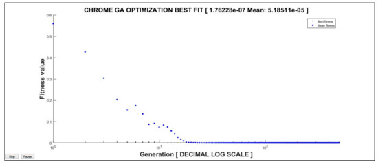
Figure 1.
Chrome GA results (first stage of optimization) for best fit across generations (500). Results are accurate in magnitude orders. Best Fit results 1.76 × 10⁻⁷ and Mean 5.19 × 10⁻⁵.
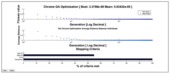
Figure 2.
Chrome GA (first stage of optimization) combined chart results for best fit across generations (700). Best fit, average distance between individuals, and stopping criteria are shown. Results are accurate. Best Fit and Mean values are lower as it was selected 700 generations.
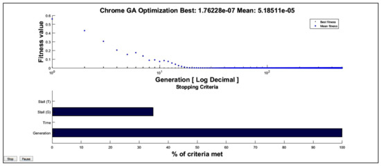
Figure 3.
Chrome GA (second stage of optimization) combined chart results for best fit across generations (500) and stopping criteria. Results are accurate in magnitude orders. Best Fit results 1.76 × 10⁻⁷ and Mean 5.19 × 10⁻⁵.
3.4. Inverse 3D Interior Tikhonov Optimization Graphical Results for Chrome
The image processing method for the 3D interior optimization results for Chrome is shown in Figure 4, Figure 5, Figure 6 and Figure 7. The numerical data that are presented in the Results section is pictured inset in the 3D charts.
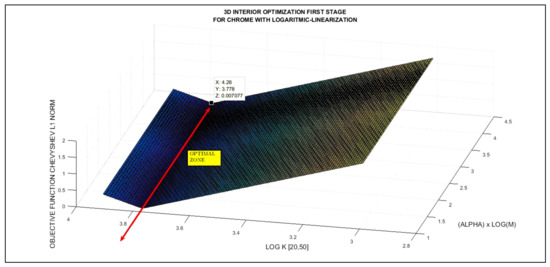
Figure 4.
Chrome first stage of 3D interior optimization. Optimal zone is accurate and OF magnitude is about 7 × 10⁻³. This value validates the chrome GA results. Optimal zone marked inset. Image processing method 1.
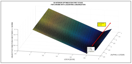
Figure 5.
Another perspective of chrome first stage of 3D interior optimization. Optimal zone is accurate and residual is about 7 × 10⁻³. This value validates the chrome GA results. Image processing method 1.
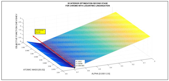
Figure 6.
Chrome second stage of 3D interior optimization. Optimal zone is accurate and OF magnitude is about 1 × 10⁻³. This value validates the chrome GA results. Subroutine for image processing is different from the first-stage 3D interior optimization charts. Image processing method 2.
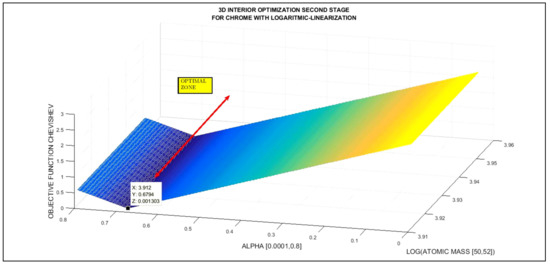
Figure 7.
Another perspective for chrome second stage of 3D interior optimization. Optimal zone is accurate and OF magnitude is about 1 × 10⁻³. This value validates the chrome GA results. Subroutine for image processing is different from the first-stage 3D interior optimization charts. Image processing method 2.
3.5. Inverse Least Squares Numerical Results for HTSC Hg-Cuprates with Molecular Effect Model
The calculation using the ILS method for the molecular effect model was conducted with two types of programs. The first was a nonlinear ILS Matlab program based on subroutines. The second was an ILS based on a polynomial fit. The best results were obtained with the second program. Table 4 shows the results for the nonlinear ILS Matlab program. Table 5 and Table 6 and Figure 8 and Figure 9 show the results of the ILS polynomial molecular effect model for the HTSC Hg-cuprates. With both methods, the different models were proved, but the polynomial one performed the best. The running time for the ILS method was about 3–6 s, including the graphics, and about 2–5 s for the ILS polynomial method.
Table 5.
Numerical results for the molecular effect model using the 6-degree polynomial method and the approximated equation. For the approximation, a quadratic polynomial is set.
Table 6.
Numerical results for the molecular effect model using the 5-degree polynomial method and the approximated equation. For the approximation, a cubic polynomial is set.
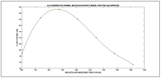
Figure 8.
Molecular effect model with ILS 6-degree polynomial fit. Generally, Tc matches a parabolic curve when the molecular weight increases.
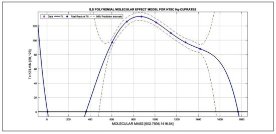
Figure 9.
Molecular effect model with ILS 5-degree polynomial fit with 96% confidence intervals. Generally, Tc matches a parabolic curve when the molecular weight increases. At lower values of molecular weight, there is a low accuracy of approximately 250 toward lower molecular weight magnitude values.
3.6. Numerical Results and Predictive Model Use Verification
The numerical validations/predictions of the optimization methods are presented in Table 7, Table 8 and Table 9. The validations are also given with the Tc and K predictions. For the molecular effect model, the 6-degree ILS numerical validation is shown in Table 9. Table 7 shows the validations/predictions for the GA chrome results. Table 8 presents the 3D/4D ILS interior optimization method validations/predictions for chrome. Table 9 shows the ILS validations/predictions for the molecular effect model for the HTSC Hg-cuprates.
Table 7.
GA program numerical results validation for chrome isotope effect model. For UAM the errors decrease.
Table 8.
3D/4D ILS interior optimization numerical validation program numerical results for chrome isotope effect model. For UAM, the errors decrease.
Table 9.
Program numerical results for molecular effect model using 6-degree polynomial and approximated equation. Errors are almost null [10−12 magnitude order]. Numerical program results for validation simulation give acceptable Tc figures. In this program, MO varied and the corresponding Tc was predicted using the model.
4. Electronics Physics and Engineering Applications
Applications of 2D/3D/4D interior and graphical optimizations [5,6,7,8,9,10,31,32,33,34,36,37,38,40,41,42,43,44] are in the field of the BCS theory of superconductivity in the isotope effect model. Further prospective applications for the molecular effect model in the HTSC groups of compounds are primarily considered for TC predictions when HTSCs show several chemical groups whose molecular composition/formulation differs in proportion to the valences/elements [5,6,7,8,9,10,31,32,33,34,36,37,38,40,41,42,43,44].
5. Discussion and Conclusions
The objective of this research was to prove/show the similarities in the results of several optimization methods applied for chrome and the HTSC-Hg-cuprates group using the BCS theory of superconductivity [2,3,4]. For chrome, the methods were the genetic algorithms and 3D/4D interior optimization methods. For the HTSC Hg-cuprates group, a hypothesis for the molecular effect model was approached and numerically analyzed. The rationale for this molecular effect model was set based on the molecules’ similar atomic weights (isotope variations in molecular composition and/or molecular approximate proportion/composition for any constituent element) for this HTSC group.
The basis for the molecular effect hypothesis has, therefore, several theoretical applications for Tc and its equation predictions. The first is a prediction of the approximate TC for a molecule whose composition within the HTSC group differs in the valence/proportion of one/several elements. The second is the case where the molecule is formed by the different isotopes of some/one of its elements, for example, any Hg isotope with a different atomic weight. The third is the case when both the theoretical and experimental facts occur, that is, when both the valence/proportion of one/several elements form part of the molecule and the type of isotopes of the molecule’s elements changes. Notably, this study sets a hypothesis/pre-hypothesis based on optimization predictions for the HTSC Hg-cuprates.
The results can be classified into numerical and 3D/2D graphical. The numerical results for the chrome isotope effect, both with GA and 3D/4D interior optimization, can be considered acceptable. Very acceptable numerical and 2D graphical optimization results using the polynomial ILS method from the HTSC Hg-cuprates molecular effect model were obtained with almost zero errors (errors about [10−3, 10−11], Table 5 and Table 6, Intel Core-3). The simple ILS method programming for the HTSC Hg-cuprate errors were higher (errors about [10−2, 10−3], Table 4).
In brief, the GA and 3D/4D interior optimization methods have verified previous studies using the 3D/4D interior optimization methods for chrome [2,3,4]. The GA method is proven as acceptable/accurate (errors about [10−6, 10−7], Table 2, Intel Core-3); the method is in parallel with the 3D/4D interior optimization method. A primary hypothesis for HTSC was tested with the Hg-cuprates group. Both the numerical and graphical results are very acceptable. However, the extension of this molecular effect model to several groups of HTSC remains to be demonstrated.
6. Scientific Ethics Standards
The advances in Interior Optimization and Graphical Optimization were created by Dr Francisco Casesnoves on 15 March 2022. The basic 2D/3D graphical optimization methods were created by Dr. Francisco Casesnoves on 3 November 2016, and the interior optimization methods in 2019. The 4D graphical and interior optimization methods were created by Dr. Francisco Casesnoves in 2020. This new GA software was originally developed by the author. This article contains information about previous papers, whose inclusion is essential to make the contribution understandable. The GA nonlinear optimization software was invented/improved based on previous contributions to subroutine modifications, patterns, loops, graphics, and optimal visualizations. In the Introduction section, the paragraph on the basic Tikhonov functional parameters was taken from [11]. The 4D interior optimization method is originally from the author (August 2021). In general, all engineering software constitutes advances/improvements from author’s series publications [2,3,4,12,13,14,15,19,20,21,22,23,24,25,26,27]. This study was carried out and the contents were investigated according to European Union Technology and Science Ethics standards in the European Textbook on Ethics in Research from the European Commission, Directorate General for Research, Unit L3, Governance and Ethics, European Research Area, Science and Society, EUR 24452 EN [45,46,47], which was based on The European Code of Conduct for Research Integrity, revised edition, ALLEA, 2017. This research was conducted entirely by the author, including the computational software used, calculations, images, mathematical propositions and statements, reference citations, and text. When a mathematical statement, proposition, or theorem is presented, a demonstration is always included. If any numerical inconsistency is determined after publication, the corresponding explanations/corrections are included in subsequent articles/books. The article is exclusively scientific, without any commercial, institutional, academic, religious, religious-similar, non-scientific theories, personal opinions, lobbies influences, friens, colleagues or relatives favours, political ideas, or economical influences. When anything is taken from a source, it is adequately recognized. Ideas and some text expressions/sentences from previous publications were emphasized with the aim of clarification [45,46,47].
Funding
This research received no external funding.
Institutional Review Board Statement
Not applicable.
Conflicts of Interest
The authors declare no conflict of interest.
References
- Vora, A.M. Modified Transition Temperature Equation for Superconductors. Chin. Phys. Lett. 2008, 25, 2162. [Google Scholar] [CrossRef]
- Casesnoves, F. Interior Optimization Methods with Electronics Applications. Int. J. Sci. Res. Sci. Eng. Technol. 2020, 7, 428–436. [Google Scholar] [CrossRef]
- Casesnoves, F. Advanced Interior Optimization Methods with Electronics Applications. Int. J. Sci. Res. Sci. Eng. Technol. 2020, 7, 97–110. [Google Scholar] [CrossRef]
- Casesnoves, F. Multiobjective Interior Optimization Computational Methods for Electronics BCS Superconductivity. Int. J. Sci. Res. Comput. Sci. Eng. Inf. Technol. 2020, 6, 280–293. [Google Scholar] [CrossRef]
- Plakida, N. High-Temperature Cuprate Superconductors Experiment, Theory, and Applications. In Springer Series in Sol-id-State Sciences; Springer: Berlin/Heidelberg, Germany, 2010; ISSN 01711873. [Google Scholar]
- Alexandrev, A.S. Theory of Superconductivity, from Weak to Strong Coupling. Series in Condensed Matter Physics; Institute of Physics Publishing: Philadelphia, PA, USA, 2003. [Google Scholar]
- Khare, N. Handbook of High-Temperature Superconductor; Marcel Dekker: New York, NY, USA, 2003; ISBN 0824708237. [Google Scholar]
- Buschow, K. Magnetic & Superconducting Materials, 2nd ed.; Elsevier: Amsterdam, The Netherlands, 2003. [Google Scholar]
- Seidel, P. Applied Superconductivity; Wiley-VCH: Hoboken, NJ, USA, 2015; Volumes 1 and 2. [Google Scholar]
- Drechsler, S.; Mishonov, T. High-T C Superconductors and Related Materials Material Science, Fundamental Properties, and Some Future Electronic Applications; Springer Science Media: Berlin/Heidenberg, Germany, 1998. [Google Scholar]
- Kazufumi, I.; Bangti, J. Inverse Problems, Tikhonov Theory and Algorithms; Series on Applied Mathematics; World Scientific: Singapore, 2015; Volume 22. [Google Scholar]
- Casesnoves, F. Mathematical Models and Optimization of Erosion and Corrosion. Ph.D. Thesis, Taltech University, Tallinn, Estonia, 14 December 2018. ISSN 25856898. [Google Scholar]
- Casesnoves, F. Die Numerische Reuleaux-Methode Rechnerische und Dynamische Grundlagen mit Anwendungen (Erster Teil); Sci-encia Scripts: Chisinau, Moldova, 2019; ISBN 139786200895608/106200895600. [Google Scholar]
- Casesnoves, F. Primary Modelling for Electromagnetic Waves Transmission in Extreme Weather Conditions. Int. J. Innov. Res. Sci. Eng. Technol. 2018, 7, 10294–10300. [Google Scholar] [CrossRef]
- Casesnoves, F. The Numerical Reuleaux Method, a Computational and Dynamical Base with Applications. First Part; Lambert Academic Publishing: Saarland, Germany, 2019; ISBN 103659917478. [Google Scholar]
- Darwin, C. The Origin of Species; Barnes & Noble Classics: New York, NY, USA, 2004. [Google Scholar]
- Haupt, R.; Haupt, S. Practical Genetic Algorithms, 2nd ed.; Wiley: New York, NY, USA, 2004. [Google Scholar]
- Abramowitz, M.; Stegun, I.A. Handbook of Mathematical Functions; U.S. Government Printing Office: Champaign, IL, USA, 1964; Volume 55.
- Casesnoves, F.; Suzenkov, A. Mathematical Models in Biotribology with 2D-3D Erosion Integral-Differential Model and Computational-Optimization/Simulation Programming. Int. J. Sci. Res. Comput. Sci. Eng. Inf. Technol. 2017, 2, 329–356, ISSN 24563307. [Google Scholar]
- Casesnoves, F.; Antonov, M.; Kulu, P. Mathematical models for erosion and corrosion in power plants. A review of appli-cable modelling optimization techniques. IEEE Xplore database and will be cross referred in SCOPUS. In Proceedings of the RUTCON2016 Power Engineering Conference, Riga, Latvia, 13 October 2016. [Google Scholar]
- Casesnoves, F. 2D computational-numerical hardness comparison between Fe-based hardfaces with WC-Co reinforcements for Integral-Differential modelling. Key Eng. Mater. J. 2018, 762, 330–338, ISSN 16629795. [Google Scholar] [CrossRef]
- Casesnoves, F.; Surzhenkov, A. Inverse methods for computational simulations and optimization of erosion models in power plants. In Proceedings of the RUTCON2017 Power Engineering Conference, Riga, Latvia, 5 December 2017. [Google Scholar] [CrossRef]
- Casesnoves, F. Computational Simulations of Vertebral Body for Optimal Instrumentation Design. J. Med. Devices 2012, 6, 021014. [Google Scholar] [CrossRef]
- Casesnoves, F. Large-Scale Matlab Optimization Toolbox (MOT) Computing Methods in Radiotherapy Inverse reatment Planning. In High Performance Computing Meeting; Nottingham University: Nottingham, UK, 2007. [Google Scholar]
- Casesnoves, F. A Monte-Carlo Optimization method for the movement analysis of pseudo-rigid bodies. In Proceedings of the 10th SIAM Conference in Geometric Design and Computing, San Antonio, TX, USA, 4–8 November 2007. Contributed Talk. [Google Scholar]
- Casesnoves, F. Applied Inverse Methods for Deformable Solid Dynamics/Kinematics in Numerical Reuleaux Method (NRM). Int. J. Numer. Methods Appl. 2013, 9, 109–131. [Google Scholar]
- Casesnoves, F. Nonlinear comparative optimization for biomaterials wear in artificial implants technology. In Proceedings of the Applied Chemistry and Materials Science RTU2018 Conference Proceedings, Rajasthan Technical University, Kota, India, 17–18 March 2018. [Google Scholar]
- Allison, J.; Amako, K.; Apotolakis, J.; Araujo, H.; Dubois, P.A.; Asai, M.; Barrand, G.; Capra, R.; Chauvie, S.; Chytracek, R.; et al. Geant4 Developments and Applications. IEEE Trans. Nucl. Sci. 2006, 53, 270–278. [Google Scholar] [CrossRef]
- Batič, M.; Hoff, G.; Pia, M.G.; Saracco, P.; Weidenspointner, G. The Geant4 Simulation Toolkit. IEEE Nucl. Sci. Symp. Med. Imaging Conf. Seoul 2013, 60, 2934–2957. [Google Scholar]
- Luenberger, G.D. Linear and Nonlinear Programming, 4th ed.; Springer: Berlin/Heidelberg, Germany, 2008. [Google Scholar]
- Huang, X. Does the isotope effect of mercury support the BCS theory? arXiv 2011, arXiv:1102.1467. [Google Scholar]
- Hummel, R.E. Electronic Properties of Materials; Springer: New York, NY, USA, 2011. [Google Scholar]
- Kasap, F.; Capper, P. (Eds.) Springer Handbook of Electronic and Photonic Materials, 4th ed.; Springer: Berlin/Heidelberg, Germany, 2000. [Google Scholar] [CrossRef]
- Kessel, W. On a General Formula for the Transition Temperature of Superconductors. Naturforschung 1974, 29a, 445–451. [Google Scholar] [CrossRef]
- Kulu, P.; Casesnoves, F.; Simson, T.; Tarbe, R. Prediction of abrasive impact wear of composite hardfacings. Solid State Phenomena. In Proceedings of 26th International Baltic Conference on Materials Engineering; Trans Tech Publications: Bäch, Swit-zerland, 2017; Volume 267, pp. 201–206. [Google Scholar] [CrossRef]
- Luiz, A. Superconductivity—Theory and Applications; InTechOpen: London, UK, 2010; ISBN 9789533071510. [Google Scholar]
- Reynolds, C.A.; Serin, B.; Nesbitt, L.B. The Isotope Effect in Superconductivity. I. Mercury. Phys. Rev. 1951, 84, 691. [Google Scholar] [CrossRef]
- Seri, B.; Reynolds, C.A.; Nesbitt, L.B. Mass Dependence of the Superconducting Transition Temperature of Mercury. Letters to Editor. Phys. Rev. 1950, 80, 761. [Google Scholar] [CrossRef]
- Todinov, M. Reliability and Risk Models; Wiley: New York, NY, USA, 2005. [Google Scholar]
- Vidyasagar, M. Nonlinear Systems Analysis, 2nd ed.; Prentice Hall: Hoboken, NJ, USA, 1993. [Google Scholar]
- Wesche, R. Chapter 50. High-Temperature Superconductors. In Springer Handbook of Electronic and Photonic Materials; Springer: Berlin/Heidelberg, Germany, 2017. [Google Scholar]
- Parinov, I.A. Microstructure and Properties of High-Temperature Superconductors, 2nd ed.; Springer: Berlin/Heidelberg, Germany, 2017. [Google Scholar]
- Fossheim, K.; Sudbø, A. Superconductivity Physics and Applications; Wiley: New York, NY, USA, 2004. [Google Scholar]
- Wang, Y.F. Fundamental Elements of Applied Superconductivity in Electrical Engineering; Wiley: New York, NY, USA, 2013. [Google Scholar]
- European Textbook on Ethics in Research. European Commission, Directorate-General for Research. Unit L3. Governance and Ethics. European Research Area. Science and Society. EUR 24452 EN. Available online: https://op.europa.eu/en/publication-detail/-/publication/12567a07-6beb-4998-95cd-8bca103fcf43 (accessed on 28 June 2021).
- ALLEA. The European Code of Conduct for Research Integrit, Revised ed.; ALLEA: Bern, Switzerland, 2017. [Google Scholar]
- Swedish Research Council. Good Research Practice; Swedish Research Council: Stockholm, Sweden, 2017; ISBN 978-91-7307-354-7. [Google Scholar]


Publisher’s Note: MDPI stays neutral with regard to jurisdictional claims in published maps and institutional affiliations. |
© 2022 by the author. Licensee MDPI, Basel, Switzerland. This article is an open access article distributed under the terms and conditions of the Creative Commons Attribution (CC BY) license (https://creativecommons.org/licenses/by/4.0/).