Abstract
This study proposes a 3D particle-based (discrete) multiphysics approach for modelling calcification in the aortic valve. Different stages of calcification (from mild to severe) were simulated, and their effects on the cardiac output were assessed. The cardiac flow rate decreases with the level of calcification. In particular, there is a critical level of calcification below which the flow rate decreases dramatically. Mechanical stress on the membrane is also calculated. The results show that, as calcification progresses, spots of high mechanical stress appear. Firstly, they concentrate in the regions connecting two leaflets; when severe calcification is reached, then they extend to the area at the basis of the valve.
1. Introduction
Aortic valve disease is the malfunction of the aortic valve due to heart malformation at birth (congenital) or developed during a lifetime related to injury, age, or calcification of the valve [1]. Calcification, in particular, may result in calcific aortic valve disease (CAVD) caused by calcium deposits on the valve leaflets, which mainly affects the elderly population with an incidence rate of 2 –7% in the population above 65 years of age [2]. Over time, calcium build-up makes the aortic valve stiffer, preventing full opening (stenosis) and hindering the blood flow from the left ventricle to the aorta. It may also prevent the valve from closing properly (regurgitation), resulting in blood leakages back to the ventricle.
Stenosis starts with the risk of leaflet deformation and progresses from early lesions to valve obstruction, which is initially mild to moderate but eventually becomes severe, with or without clinical symptoms [3] and the patient has high risk of cardiac failure.
In the literature, several studies focus on the dynamics of blood flow and the deformation of the calcified aortic valve leaflets to better understand and assess the severity of calcification. Computational fluid dynamics (CFD) was used to generate patient-specific aortic valve models from patients’ medical images in [4,5]. Other studies [6,7,8,9,10] focus on investigating the stresses on the valve leaflets, excluding the fluid flow behaviour in the model. Since the behaviour of the aortic valve depends on both the fluid and the leaflets, a fluid–structure interaction (FSI) approach is recommended to model the complex dynamic of this problem [2,11].
In this paper, we aim to use discrete multiphysics (DMP) [12,13,14], which enables the fluid–solid interaction, to develop a 3D model representing various stages of calcification of the aortic valve. DMP has been extensively used in in silico medicine for modelling a variety of human systems including the aortic valve [15], the intestine [16], deep venous valves [17,18], the lungs [19], and, in conjunction with machine learning, peristalsis in the oesophagus [20]. Section 2 and Section 3 give an overview of the method and model used, respectively.
2. Discrete Multiphysics
Multiphysics simulation allows for tackling problems that involve multiple physical models or simultaneous physical phenomena, and that gives it widespread application in both industry and academia [20]. Discrete multiphysics, therefore, is a method based on particles and that combines various particle methods such as smoothed particle hydrodynamics (SPH), lattice spring model (LSM), and discrete element method [15]. The current model only accounts for SPH and LSM. Both modelling techniques are briefly discussed below. The reader can refer to [21] for a more extensive introduction to SPH, and to [22] for the LSM. Details on how the two models are linked together in DMP can be found in [12,13].
2.1. Smooth Particle Hydrodynamics
Smoothed particle hydrodynamics (SPH) was invented to simulate nonaxisymmetric phenomena in astrophysics by [23,24] and to solve the astrophysical problems in three-dimensional open space [24]. It is a meshless Lagrangian particle method used to solve differential equations which are often found in engineering and scientific problems [25,26]. The method, being easy to work with a reasonable degree of accuracy, could be extended to complicated physics without much trouble [27]. The SPH method is gaining popularity in a variety of fields and has a wide range of applications such as multiphase flow [25,28], biomedicals [15,17,19,29], fluid–solid interaction [12,29,30,31,32,33], and hydrodynamic instability [34,35].
The SPH method represents the state of a system with particles which possess individual material properties and move according to a governing equation [36]. The fundamental idea behind this discrete approximation lies in the mathematical identity
which gives a discretized particle approximation within a domain of a smoothing function (kernel) W within a characteristic width h called the smoothing length [12] such that
This gives rise to the discrete approximation
which can be discretised over a series of particle of mass mi and density ρi to obtain
where f(r) is a generic function defined over the volume V, r is the three-dimensional vector point, and δ(r) is the three-dimensional delta function.
Equation (4) is a representation of the discrete approximation of a generic continuous field. Further simplification of Equation (4) can be done to approximate the Navier–Stokes equation. See detail and complete equations in [14,15]. In addition, more information on the SPH and equation derivation can also be found in [21,35,37].
2.2. Lattice Spring Model (LSM)
The behaviour of deformable objects can be simulated using the LSM approach. This model consists of mass point and linear springs which exert forces at the nodes located at the end point [38], which are placed on either a regular lattice or positioned randomly within the system [38]. The term LSM is interchangeable with mass spring model (MSM), where the latter is mostly used in computer graphics and the former in solid mechanics. Nowadays, LSM is applicable in many areas and disciplines, for instance, cloth simulation, face animation, or soft tissue behaviour in surgery training systems [39,40] are simulated using LSM.
The LSM follows the idea that any material point of the body can be referred to by its position vector r = (x,y,z) [38]. When that body undergoes deformation due to an applied force F, the displacement is proportional to the force applied.
where r0 is the initial distance between the two particles, r is the distance at time t, and k is a Hookean constant
3. The Model
As mentioned, the multiphysics model used in this study is based on DMP, a computational method that combines various particle methods. In the case under investigation, the computational domain is divided into two parts: (i) a liquid part (blood) where smooth particle hydrodynamics (SPH) is used, and (ii) the solid structure part (valve) where the stress deformation equation is solved using the lattice spring model (LSM). The two parts are coupled together to represent an FSI model that simulates the valve deformation and blood flow dynamics within the valve.
In Figure 1a, the valve’s leaflets (tricuspid) are shown; Figure 1b shows the overall geometry. The geometry was firstly designed as a CAD model (nodes and elements) and then transformed to a particle model as explained in the Appendix A. Simulations were run with the open-source software LAMMPS [41].
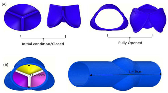
Figure 1.
Valve leaflets (a) and complete geometry (b).
The system is three-dimensional and consists of 418,743 particles: 342,358 particles for the fluid, 19,725 particles for the leaflets, and 56,660 particles for the rigid pipe. The distance between particles (particle spacing) and the number of particles were chosen from the previous work done where DMP was used to model similar FSI problems [29,32]. In this study, the aortic valve geometry of Bavo et al. (2016) was adopted. The leaflets tissue was modelled as linear and elastic, whereas the elasticity of the aorta (rigid pipe) was neglected and the arterial wall was assumed to be rigid [42].
In the simulation, the flow is driven by a periodic acceleration (Figure 2) given by
where G0 = 400 m s−2, ω = 2πf is the angular frequency, n = 13, and ϕ = π/10 as discussed in Steven et al., 2003 [40]. The value of G0 is determined to achieve full opening of the valve that gives an average flow rate around 600 mL s−1 for valves at normal condition, which is consistent with the literature, e.g., [40,43,44].
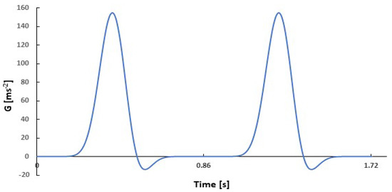
Figure 2.
Pulsatile flow function.
As mentioned, the flexible valve is modelled with LSM, which is a common approach for cardiovascular valves [45]. This implies that each computational particle is linked with its neighbour particles by means of a force (in Equation (5)).
In LSM, the value of k is linked to the Young modulus E of the material [38]. In practice, however, it is not always straightforward to calculate k from E in the case of complex geometries, in particular, with irregular particles distribution [39]. For this reason, we use a more practical approach: k is determined, together with G0, in such a way that the valve opens fully and the flow rate for a healthy and non-calcified valve is 600 mL s−1 as discussed above.
The numerical model used in this paper has extensively been tested and validated for a variety of similar fluid flow problems [15,16,17,18,32]. In this paper, the value of k in the lattice model, as mentioned earlier, and G0 in Equation (6) were chosen in such a way to make sure the flow in the valve and its opening are consistent with available observations (e.g., [40,43,44,46,47]). Convergence of the results on the number of particles used to discretise the system was carried out and the numbers reported in Table 1 represent the best compromise between accuracy and computational times. Since we refer to the human body, the available observations of real valves show very scattered results because of individual variability. Therefore, we cannot provide a systematic validation like in the case of experiments carried out in a laboratory under controlled conditions. This is even more true for calcified valves, where, on top of physiological variations, we have additional variations due to the severity and the course of the disease. Given all of the above, the best we can do is to make sure that the results are consistent with real data. In our study, we achieved this by making sure that the flow in the valve and the opening of the leaflets are both within the range of real observations.

Table 1.
Model parameters used in the simulation; for the meaning of SPH parameters such as α or h, refer to Liu and Liu, 2003 [21].
4. Results and Discussion
4.1. Stages of Calcification
In our model, the value of k was chosen to control the stiffness of the valve and model calcification. The higher the value of k, the stiffer the valve. In our model, higher values of k are used to model a higher degree of calcification. We define the degree of calcification γ as
where k is the spring constant used to simulate the calcified valve and kH is the stiffness of the healthy valve. Figure 3 shows the valve during maximal opening for four different degrees of calcification.
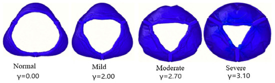
Figure 3.
Severity of aortic valve stenosis in terms of orifice opening (stenosis).
Some important parameters like flow velocity, volume flow rate, and stress can be used to ascertain the level of calcification of the valves. Figure 4 shows how the flow velocity in the valve is affected by calcification.
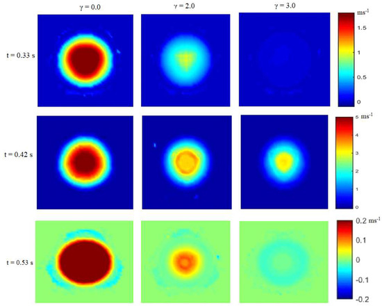
Figure 4.
Velocity profile at different time steps.
The flow velocity was measured on a section just above the valve for three different degrees of calcification and three different times. According to the level of calcification, the valve opens and closes at different times. The healthy valve (γ = 0) starts opening at t = 0.29 s, reaches maximal opening (peak systole) at t = 0.41 s, and closes again at t = 0.56 s. The valve with γ = 2.0 starts opening at t = 0.32 s, reaches maximal opening at t = 0.43 s, and closes again at t = 0.54 s. The valve with γ = 3.0 starts opening at t = 0.37 s, reaches maximal opening at t = 0.43 s, and closes again at t = 0.53 s. Figure 4 also relates with Figure 3 in showing how the valve opening is reduced (stenosis) in case of calcification. The time to attain peak velocity varies with the severity of the valve’s stenosis, which signifies high mortality risk and the need for a valve replacement [48]. The time at which the valve closes also varies with the severity of calcification; at γ = 3.0, there is also evidence of regurgitation (back flow), a characteristic of a stenotic aortic valve [2,3,9]. Figure 4 also shows that, as expected, the blood flow in the healthy valve (γ = 0.0) is higher than in the calcified valves (γ = 2.0 and γ = 3).
Transvalvular flow is another important parameter for measuring aortic valve functionality. The flow reduces as γ increases (Figure 5); it decreases almost linearly up to a critical value γCR = 3, after which it decreases sharply. In Figure 5, γCR corresponds to a flow rate of 200 mL s−1. Our calculations are consistent with the medical literature where a flow rate ≥250 mL s−1 is considered acceptable, whereas <200 mL s−1 is associated with an increase of mortality rate in cases of patients with aortic stenosis [44,49]. The maximum orifice diameter and the average stress on the valve (see next section) can also be used to monitor the progression of the valve stenosis. Table 2 summarizes the parameters as the condition worsens from normal to severe.
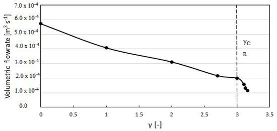
Figure 5.
Volumetric blood flow with respect to γ.
Table 2.
Parameters for determining severity of calcification.
4.2. Stress Distribution on the Membrane
Calcification increases the stiffness of the valve, which results in higher stresses on the membrane. This is particularly important because mechanical stress plays a major role in the calcification of bioprostheses [50]. This, potentially, can create a vicious circle where calcification leads to higher mechanical stress, which, in turn, leads to further calcification. Figure 6 shows how the average stress increases with the degree of calcification. Since stenosis due to calcification can be related to congenital bicuspid valve disease or fused leaflets [51], the numerical values of 0.28 to 0.35 MPa obtained for calcified valves are consistent with those reported by [46] for fused tri-leaflet valves. For stress distribution in a transcatheter aortic valve, the maximum value of 0.35 MPa is also consistent with the report of Auricchio et al. (2014) [47].
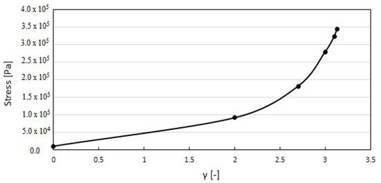
Figure 6.
Stress at different degrees of calcification.
The local stress distribution (i.e., the Frobenius norm of the stress tensor) on the leaflets is shown in Figure 7, considering a membrane thickness of 0.6 mm [7]. In this work, calcification is modelled by uniformly increasing the Young modulus of the membrane; Figure 7 suggests that calcification does not progress uniformly.
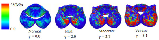
Figure 7.
Mechanical stress on the valve leaflets at maximal opening.
In fact, as calcification progresses, spots of high mechanical stress appear. Firstly, they concentrate in the regions connecting two leaflets; when severe calcification is reached, they extend to the area at the basis of the valve.
5. Conclusions
In this study, the effect of calcification in a 3D aortic valve is simulated with discrete multiphysics. The model accounts for both hemodynamics and leaflet deformation, and it can be considered an improvement over a previous 2D model [15]. The results show that the mean transvalvular flow could be used to assess valve calcification, and severe calcification occurs when the flow rate is lower than 200 mL s−1.
The model can also assess the local stress on the membrane. Calcification increases mechanical stress, which, in turn, promotes further calcification. In this work, calcification is modelled by uniformly increasing the Young modulus of the membrane. The results show that, as calcification progresses, spots of high mechanical stress appear. Firstly, they concentrate in the regions connecting two leaflets; when severe calcification is reached, they extend to the area at the basis of the valve. This suggests that the model could be improved by accounting for local changes in stiffness, which depends on the local stress distribution.
Methodologically, this work can also benefit researchers interested in particle methods, but not necessarily to cardiovascular applications. In fact, the Appendix A explains how geometries designed with CAD model can be transformed to particle models.
Author Contributions
Conceptualization, A.A., A.M.M., and M.A.; simulation and visualization, A.M.M.; numerical calculations, A.M.M.; interpretation and analysis of results, A.M.M. and A.A.; writing—original draft preparation, A.M.M.; supervision, A.A.; writing—review and editing, A.A., A.M.M., and M.A.; input script, M.A. and A.A.; model and appendix, M.A. All authors have read and agreed to the published version of the manuscript.
Funding
This research received no external funding.
Acknowledgments
The Nigerian Petroleum Technology Development Fund (PTDF) is acknowledged for the provision of a scholarship to Adamu Musa Mohammed.
Conflicts of Interest
The authors declare no conflict of interest.
Appendix A
This appendix explains how to adapt the 3D CAD model for Discrete Multiphysics. The valve geometry is taken from [42] and was initially created with the help of CAD software. In general, particle distribution can be generated with a programming code or a pre-processing solver. In the first case, the coordinates of the points are created with a separate standard programming code such as C++ and MATLAB, or directly in the processing solver with an integrated algorithm (in the software LAMMPS for instance). For complex geometries, a pre-processing commercial builder (GAMBIT, ABAQUS, SALOME) can be used for the structure and the associated mesh is then replaced with particles (Figure A1). In the paper, we used the second approach in order to design our tricuspid valve system.

Figure A1.
Mesh generation using a pre-processing solver (a) and the generated particle distribution (b).
Figure A1.
Mesh generation using a pre-processing solver (a) and the generated particle distribution (b).

The procedure of implementation is simple, but it requires a couple of sequences to obtain the final input file. Here, we present the one used for our valve model, but the methodology can be extended to any other applications.
The different steps can be described as follow:
- Creation or importation of the CAD geometry
- Writing of the data file
- Generation of the bond and coefficient files
- Implementation of the input file
The first step consists of designing the part geometry or importing an existing one to any CAD commercial or open-source software (Figure A2a). The idea is to use the software capability for automatically or manually generating the mesh (elements and nodes, Figure A2b). Next, the nodes information (numbers and coordinates) are downloaded (Figure A2c) and collected into a text file (Figure A2d).
Subsequently, the data file is adapted and implemented in a LAMMPS format file, which contains specific line codes and keywords (for more details and documentation, readers can refer to the LAMMPS documentation available at https://lammps.sandia.gov/doc/Manual.html). For instance, for this model, we used the keywords meso for the atom style and bond for the inter-atomic potential.
The unsymmetrical shape of the tricuspid valve system makes a 3D design necessary. This representation requires a fine mesh with a consequent number of nodes (418,743 particles) to ensure a realistic valve motion. Each node/particle is connected with at least three other nodes located nearby, increasing the data processing drastically. As a result, we developed an algorithm (C++ code) in order to set the bond definitions automatically. All particle positions are scanned by the code and for each particle, its neighbour (within a prescribed radius distance of interaction) is identified, numbered, and printed out in a bond file. Meanwhile, a second file is also created with the storage of the bond coefficients (potential force) and the distance (between two particles).
Finally, as the number of fluid particles is very important (342,358), the inclusion of the list into the data file (which is technically possible) makes the input file processing heavy. Instead, we preferred to generate, during the first step of the simulation, the fluid particles via the LAMMPS commands ‘create_atoms’ and ‘region’. The command ‘delete’ is also used to avoid overlapping.

Figure A2.
Tricuspid valve CAD part (a), tricuspid valve meshed CAD part (b), nodes generation using the CAD software (c), and external data file (d).
Figure A2.
Tricuspid valve CAD part (a), tricuspid valve meshed CAD part (b), nodes generation using the CAD software (c), and external data file (d).

References
- Fioretta, E.S.; Dijkman, P.E.; Emmert, M.Y.; Hoerstrup, S.P. The Future of Heart Valve Replacement: Recent Developments and Translational Challenges for Heart Valve Tissue Engineering: The Future of Heart Valve Replacement. J. Tissue Eng. Regen. Med. 2018, 12, e323–e335. [Google Scholar] [CrossRef] [PubMed]
- Amindari, A.; Saltik, L.; Kirkkopru, K.; Yacoub, M.; Yalcin, H.C. Assessment of Calcified Aortic Valve Leaflet Deformations and Blood Flow Dynamics Using Fluid-Structure Interaction Modeling. Inform. Med. Unlocked 2017, 9, 191–199. [Google Scholar] [CrossRef]
- Otto, C.M.; Prendergast, B. Aortic-Valve Stenosis—From Patients at Risk to Severe Valve Obstruction. N. Engl. J. Med. 2014, 371, 744–756. [Google Scholar] [CrossRef] [PubMed]
- Fedele, M.; Faggiano, E.; Dedè, L.; Quarteroni, A. A Patient-Specific Aortic Valve Model Based on Moving Resistive Immersed Implicit Surfaces. Biomech. Modeling Mechanobiol. 2017, 16, 1779–1803. [Google Scholar] [CrossRef] [PubMed]
- Youssefi, P.; Gomez, A.; He, T.; Anderson, L.; Bunce, N.; Sharma, R.; Figueroa, C.A.; Jahangiri, M. Patient-Specific Computational Fluid Dynamics—Assessment of Aortic Hemodynamics in a Spectrum of Aortic Valve Pathologies. J. Thorac. Cardiovasc. Surg. 2017, 153, 8–20. [Google Scholar] [CrossRef] [PubMed]
- Bluestein, D.; Einav, S. The Effect of Varying Degrees of Stenosis on the Characteristics of Turbulent Pulsatile Flow through Heart Valves. J. Biomech. 1995, 28, 915–924. [Google Scholar] [CrossRef]
- Hamid, M.S.; Sabbah, H.N.; Stein, P.D. Comparison of Finite Element Stress Analysis of Aortic Valve Leaflet Using Either Membrane Elements or Solid Elements. Comput. Struct. 1985, 20, 955–961. [Google Scholar] [CrossRef]
- Arjunon, S.; Rathan, S.; Jo, H.; Yoganathan, A.P. Aortic Valve: Mechanical Environment and Mechanobiology. Ann. Biomed. Eng. 2013, 41, 1331–1346. [Google Scholar] [CrossRef]
- Morganti, S.; Conti, M.; Aiello, M.; Valentini, A.; Mazzola, A.; Reali, A.; Auricchio, F. Simulation of Transcatheter Aortic Valve Implantation through Patient-Specific Finite Element Analysis: Two Clinical Cases. J. Biomech. 2014, 47, 2547–2555. [Google Scholar] [CrossRef]
- Lazaros, G.; Drakopoulou, M.I.; Tousoulis, D. Transaortic Flow in Aortic Stenosis: Stroke Volume Index versus Flow Rate. Cardiology 2018, 141, 71–73. [Google Scholar] [CrossRef]
- Ghasemi Bahraseman, H.; Mohseni Languri, E.; Yahyapourjalaly, N.; Espino, D.M. Fluid-Structure Interaction Modeling of Aortic Valve Stenosis at Different Heart Rates. Acta Bioeng. Biomech. 2016, 18, 11–20. [Google Scholar] [CrossRef]
- Alexiadis, A. The Discrete Multi-Hybrid System for the Simulation of Solid-Liquid Flows. PLoS ONE 2015, 10, e0124678. [Google Scholar] [CrossRef] [PubMed]
- Alexiadis, A. A Smoothed Particle Hydrodynamics and Coarse-Grained Molecular Dynamics Hybrid Technique for Modelling Elastic Particles and Breakable Capsules under Various Flow Conditions: SPH-CGMD HYBRID. Int. J. Numer. Meth. Eng. 2014, 100, 713–719. [Google Scholar] [CrossRef]
- Alexiadis, A. A New Framework for Modelling the Dynamics and the Breakage of Capsules, Vesicles and Cells in Fluid Flow. Procedia IUTAM 2015, 16, 80–88. [Google Scholar] [CrossRef]
- Ariane, M.; Allouche, M.H.; Bussone, M.; Giacosa, F.; Bernard, F.; Barigou, M.; Alexiadis, A. Discrete Multi-Physics: A Mesh-Free Model of Blood Flow in Flexible Biological Valve Including Solid Aggregate Formation. PLoS ONE 2017, 12, e0174795. [Google Scholar] [CrossRef]
- Alexiadis, A.; Stamatopoulos, K.; Wen, W.; Batchelor, H.K.; Bakalis, S.; Barigou, M.; Simmons, M.J.H. Using Discrete Multi-Physics for Detailed Exploration of Hydrodynamics in an In Vitro Colon System. Comput. Biol. Med. 2017, 81, 188–198. [Google Scholar] [CrossRef]
- Ariane, M.; Vigolo, D.; Brill, A.; Nash, F.G.B.; Barigou, M.; Alexiadis, A. Using Discrete Multi-Physics for Studying the Dynamics of Emboli in Flexible Venous Valves. Comput. Fluids 2018, 166, 57–63. [Google Scholar] [CrossRef]
- Ariane, M.; Wen, W.; Vigolo, D.; Brill, A.; Nash, F.G.B.; Barigou, M.; Alexiadis, A. Modelling and Simulation of Flow and Agglomeration in Deep Veins Valves Using Discrete Multi Physics. Comput. Biol. Med. 2017, 89, 96–103. [Google Scholar] [CrossRef]
- Ariane, M.; Kassinos, S.; Velaga, S.; Alexiadis, A. Discrete Multi-Physics Simulations of Diffusive and Convective Mass Transfer in Boundary Layers Containing Motile Cilia in Lungs. Comput. Biol. Med. 2018, 95, 34–42. [Google Scholar] [CrossRef]
- Alexiadis, A. Deep Multiphysics: Coupling Discrete Multiphysics with Machine Learning to Attain Self-Learning in-Silico Models Replicating Human Physiology. Artif. Intell. Med. 2019, 98, 27–34. [Google Scholar] [CrossRef]
- Liu, G.R.; Liu, M.B. Smoothed Particle Hydrodynamics: A Meshfree Particle Method; World Scientific: Hackensack, NJ, USA, 2003. [Google Scholar]
- Kot, M.; Nagahashi, H.; Szymczak, P. Elastic Moduli of Simple Mass Spring Models. Vis. Comput. 2015, 31, 1339–1350. [Google Scholar] [CrossRef]
- Gingold, R.A.; Monaghan, J.J. Smoothed Particle Hydrodynamics: Theory and Application to Non-Spherical Stars. Mon. Not. R. Astron. Soc. 1977, 181, 375–389. [Google Scholar] [CrossRef]
- Lucy, L.B. A Numerical Approach to the Testing of the Fission Hypothesis. Astron. J. 1977, 82, 1013. [Google Scholar] [CrossRef]
- Hopp-Hirschler, M.; Shadloo, M.S.; Nieken, U. A Smoothed Particle Hydrodynamics Approach for Thermo-Capillary Flows. Comput. Fluids 2018, 176, 1–19. [Google Scholar] [CrossRef]
- Shadloo, M.S.; Zainali, A.; Sadek, S.H.; Yildiz, M. Improved Incompressible Smoothed Particle Hydrodynamics Method for Simulating Flow around Bluff Bodies. Comput. Methods Appl. Mech. Eng. 2011, 200, 1008–1020. [Google Scholar] [CrossRef]
- Monaghan, J.J. Smoothed Particle Hydrodynamics. Annu. Rev. Astron. Astrophys. 1992, 30, 543–574. [Google Scholar] [CrossRef]
- Rahmat, A.; Yildiz, M. A Multiphase ISPH Method for Simulation of Droplet Coalescence and Electro-Coalescence. Int. J. Multiph. Flow 2018, 105, 32–44. [Google Scholar] [CrossRef]
- Schütt, M.; Stamatopoulos, K.; Simmons, M.J.H.; Batchelor, H.K.; Alexiadis, A. Modelling and Simulation of the Hydrodynamics and Mixing Profiles in the Human Proximal Colon Using Discrete Multiphysics. Comput. Biol. Med. 2020, 121, 103819. [Google Scholar] [CrossRef]
- Ji, S.; Chen, X.; Liu, L. Coupled DEM-SPH Method for Interaction between Dilated Polyhedral Particles and Fluid. Math. Probl. Eng. 2019, 2019, 1–11. [Google Scholar] [CrossRef]
- Li, D.; Zhen, Z.; Zhang, H.; Li, Y.; Tang, X. Numerical Model of Oil Film Diffusion in Water Based on SPH Method. Math. Probl. Eng. 2019, 2019, 1–14. [Google Scholar] [CrossRef]
- Rahmat, A.; Barigou, M.; Alexiadis, A. Deformation and Rupture of Compound Cells under Shear: A Discrete Multiphysics Study. Phys. Fluids 2019, 31, 051903. [Google Scholar] [CrossRef]
- Tran-Duc, T.; Phan-Thien, N.; Khoo, B.C. A Smoothed Particle Hydrodynamics (SPH) Study of Sediment Dispersion on the Seafloor. Phys. Fluids 2017, 29, 083302. [Google Scholar] [CrossRef]
- Rahmat, A.; Tofighi, N.; Shadloo, M.S.; Yildiz, M. Numerical Simulation of Wall Bounded and Electrically Excited Rayleigh–Taylor Instability Using Incompressible Smoothed Particle Hydrodynamics. Colloids Surf. A Physicochem. Eng. Asp. 2014, 460, 60–70. [Google Scholar] [CrossRef]
- Shadloo, M.S.; Yildiz, M. Numerical Modeling of Kelvin-Helmholtz Instability Using Smoothed Particle Hydrodynamics. Int. J. Numer. Meth. Engng. 2011, 87, 988–1006. [Google Scholar] [CrossRef]
- Liu, M.B.; Liu, G.R. Restoring Particle Consistency in Smoothed Particle Hydrodynamics. Appl. Numer. Math. 2006, 56, 19–36. [Google Scholar] [CrossRef]
- Shadloo, M.S.; Zainali, A.; Yildiz, M. Simulation of Single Mode Rayleigh–Taylor Instability by SPH Method. Comput. Mech. 2013, 51, 699–715. [Google Scholar] [CrossRef]
- Pazdniakou, A.; Adler, P.M. Lattice Spring Models. Transp. Porous. Med. 2012, 93, 243–262. [Google Scholar] [CrossRef]
- Lloyd, B.; Szekely, G.; Harders, M. Identification of Spring Parameters for Deformable Object Simulation. IEEE Trans. Visual. Comput. Graph. 2007, 13, 1081–1094. [Google Scholar] [CrossRef]
- Stevens, S.A.; Lakin, W.D.; Goetz, W. A Differentiable, Periodic Function for Pulsatile Cardiac Output Based on Heart Rate and Stroke Volume. Math. Biosci. 2003, 182, 201–211. [Google Scholar] [CrossRef]
- Plimpton, S. Fast Parallel Algorithms for Short-Range Molecular Dynamics. J. Comput. Phys. 1995, 117, 1–19. [Google Scholar] [CrossRef]
- Bavo, A.M.; Rocatello, G.; Iannaccone, F.; Degroote, J.; Vierendeels, J.; Segers, P. Fluid-Structure Interaction Simulation of Prosthetic Aortic Valves: Comparison between Immersed Boundary and Arbitrary Lagrangian-Eulerian Techniques for the Mesh Representation. PLoS ONE 2016, 11, e0154517. [Google Scholar] [CrossRef] [PubMed]
- Murgo, J.P.; Westerhof, N.; Giolma, J.P.; Altobelli, S.A. Aortic Input Impedance in Normal Man: Relationship to Pressure Wave Forms. Circulation 1980, 62, 105–116. [Google Scholar] [CrossRef] [PubMed]
- Blais, C.; Burwash, I.G.; Mundigler, G.; Dumesnil, J.G.; Loho, N.; Rader, F.; Baumgartner, H.; Beanlands, R.S.; Chayer, B.; Kadem, L.; et al. Projected Valve Area at Normal Flow Rate Improves the Assessment of Stenosis Severity in Patients With Low-Flow, Low-Gradient Aortic Stenosis: The Multicenter TOPAS (Truly or Pseudo-Severe Aortic Stenosis) Study. Circulation 2006, 113, 711–721. [Google Scholar] [CrossRef]
- Hammer, P.E.; Sacks, M.S.; del Nido, P.J.; Howe, R.D. Mass-Spring Model for Simulation of Heart Valve Tissue Mechanical Behavior. Ann. Biomed. Eng. 2011, 39, 1668–1679. [Google Scholar] [CrossRef] [PubMed]
- Jermihov, P.N.; Jia, L.; Sacks, M.S.; Gorman, R.C.; Gorman, J.H.; Chandran, K.B. Effect of Geometry on the Leaflet Stresses in Simulated Models of Congenital Bicuspid Aortic Valves. Cardiovasc. Eng. Tech. 2011, 2, 48–56. [Google Scholar] [CrossRef] [PubMed]
- Auricchio, F.; Conti, M.; Morganti, S.; Reali, A. Simulation of Transcatheter Aortic Valve Implantation: A Patient-Specific Finite Element Approach. Comput. Methods Biomech. Biomed. Eng. 2014, 17, 1347–1357. [Google Scholar] [CrossRef] [PubMed]
- Kamimura, D.; Hans, S.; Suzuki, T.; Fox, E.R.; Hall, M.E.; Musani, S.K.; McMullan, M.R.; Little, W.C. Delayed Time to Peak Velocity Is Useful for Detecting Severe Aortic Stenosis. JAHA 2016, 5. [Google Scholar] [CrossRef]
- Saeed, S.; Senior, R.; Chahal, N.S.; Lønnebakken, M.T.; Chambers, J.B.; Bahlmann, E.; Gerdts, E. Lower Transaortic Flow Rate Is Associated with Increased Mortality in Aortic Valve Stenosis. JACC Cardiovasc. Imaging 2017, 10, 912–920. [Google Scholar] [CrossRef]
- Thubrikar, M.; Deck, J.; Aouad, J.; Nolan, S. Role of Mechanical Stress in Calcification of Aortic Bioprosthetic Valves. J. Thorac. Cardiovasc. Surg. 1983, 86, 115–125. [Google Scholar] [CrossRef]
- Huntley, G.D.; Thaden, J.J.; Alsidawi, S.; Michelena, H.I.; Maleszewski, J.J.; Edwards, W.D.; Scott, C.G.; Pislaru, S.V.; Pellikka, P.A.; Greason, K.L.; et al. Comparative Study of Bicuspid vs. Tricuspid Aortic Valve Stenosis. Eur. Heart J. Cardiovasc. Imaging 2018, 19, 3–8. [Google Scholar] [CrossRef]


© 2020 by the authors. Licensee MDPI, Basel, Switzerland. This article is an open access article distributed under the terms and conditions of the Creative Commons Attribution (CC BY) license (http://creativecommons.org/licenses/by/4.0/).