Abstract
This paper aims to present efficient efforts to optimize the proportional-integral-differential (PID) controller of clinker cooling in grate coolers, which have a fixed grate and at least two moving ones. The process model contains three transfer functions between the speed of the moving grate and the pressures of the static and moving grates. The developed software achieves the identification of the model parameters using industrial data and by implementing non-linear regression methods. The design of the PID controller follows a loop-shaping technique, imposing as a constraint the maximum sensitivity, Ms, of the open-loop transfer function and providing a set of PIDs that satisfy a range of Ms. A simulator determines the optimal PID sets among those calculated at the design step using the integral of absolute error (IAE) as a performance criterion. The combination of a robustness constraint with a performance criterion, Ms and IAE respectively, leads to an area of controllers with Ms belonging to the range of 1.2 to 1.35. The IAE is between 4.2% and 4.8%, depending on the set-point value. PID sets located near the middle of this area can be chosen and implemented in the cooler’s routine operation.
1. Introduction
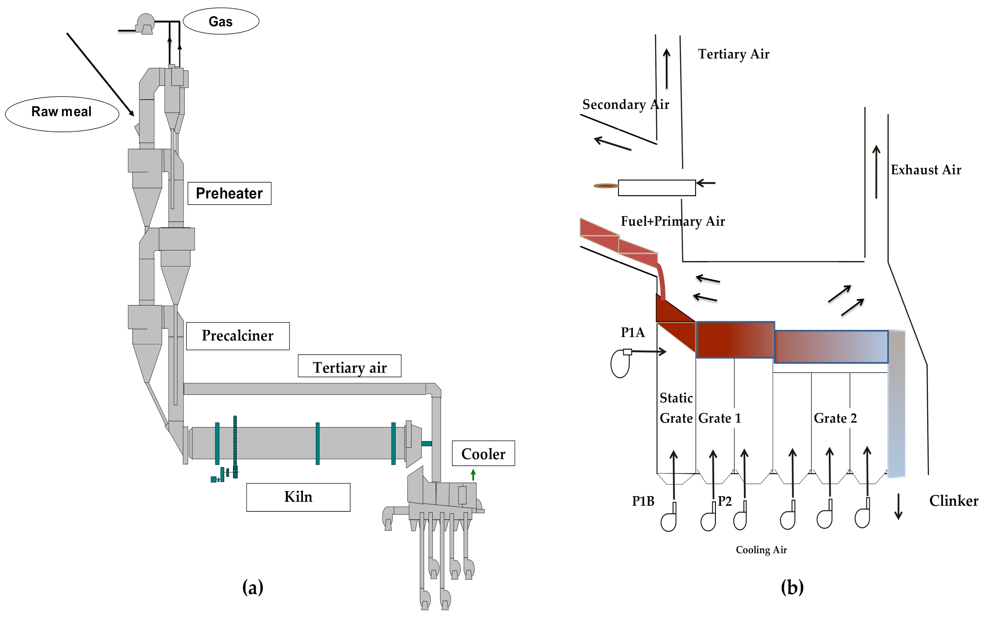
Grate coolers constitute a key component of the clinker’s dry production lines, having the rapid cooling of clinker and heat recovery as their main function. The stability degree of the cooler’s operation affects both the performance of the entire burning line and the product’s quality. A simplified representation of the flows and the basic components of a rotary kiln (RK) is demonstrated in Figure 1a. The raw meal, consisting mainly of ground limestone and clay, is fed to the preheater, where it is heated and partially calcined by the hot gases from the kiln and the pre-calciner in an anti-current flow. The decomposed material enters the kiln, where after the calcination is completed, it is transformed into clinker. The air volumes needed for the calcination and combustion come from the primary, secondary, and tertiary air. Τhe very hot clinker then falls onto the grates of the cooler through the hood of the kiln and is cooled by air streams passing vertically from the grates. The cooler includes a fixed grate and at least two moving ones. Figure 1b shows a simplified graphic of a grate cooler. Due to their oscillating motion, the grates cause the solid material to flow forward and spread. After the final moving grate, clinker is first passed through a crusher and then transferred to the corresponding silo.

Figure 1.
Simplified representation of (a) rotary kiln installation; (b) grate cooler.
During clinker cooling, a heat exchange occurs between the solid material and vertically incoming fresh air. A part of the hot air volume enters the kiln as secondary air, another part is led to the pre-calciner, and the remaining goes towards the de-dusting filter as exhaust air. The effectiveness of clinker cooling is linked to two factors: (a) the recovery of heat from the material entering the cooler and (b) its cooling rate, because rapid cooling helps to increase the quality of the product [1]. Another particularly important goal is to keep the temperatures and flow rates of the secondary and tertiary air as stable as possible because any significant disturbance to them affects kiln operation. The above is possible by controlling and stabilizing the thickness of the clinker bed on the first moving grate, taking into account that this thickness depends on the speed of the grate and the mass flow rate from the kiln. Because the latter cannot be controlled by the cooler, as any change is a disturbance, the only control variable is the speed of the first moving grate. The primary air is also not controlled by the cooler. It is fed to the main burner with the fuel and determines the shape of the flame. Subsequent grates usually move 10–20% faster than the first one.
For a very thick layer, cooling air cannot blow through the clinker, the cooling is uneven, and the clinker remains too hot at the outlet of the cooler. In the case of a thin layer, the air passes rapidly through it and the heat recovery is poor, resulting in reduced temperatures of secondary and tertiary air. In addition, there is a risk of damage to the grate’s plates if a very hot wave of clinker comes from the kiln, so a sufficient material thickness protects the cooler. In practice, reliable continuous measurement of bed thickness is difficult. For this reason, the pressure under the first moving grate is used, considered as proportional to the bed’s layer on the grate, as the process variable. The latter also depends on the flow rate of air entering the grate. In most cases, in industrial practice, the speed of cooling fans remains relatively constant and is regulated only under specific conditions. Thus, the main loop of the cooler’s automatic control, in an attempt to attenuate disturbances, is between the speed and the pressure of the first moving grate. In most automation systems in modern cement plants, conventional proportional-integral-differential (PID) controllers are installed in the subsystem of the clinker cooling, using the previous loop. The difficulty arises in finding optimal or at least satisfactory values of the PID parameters, which adequately regulate the grate pressure. In the process control, more than 95% of the control loops are of PID type [2] (p. 1). Astrom [3] clearly stated that a central theme in automatic control is model uncertainty and robustness. Therefore, the automatic control of the cooler requires a reliable model, which includes control and process variables, as well as variables that describe disturbances and noises entering the system. In terms of dynamic parameters, both their mean values and uncertainty are equally necessary.
Tsamatsoulis [4] developed a simplified dynamic model of clinker cooling. He modeled the response of three different pressures to changes in the speed of the moving grate using time-delayed integral transfer functions and long-term industrial data. The simplified transfer functions indicate that there is some effect of the speed of the moving grate on the pressure of the fixed one. However, the modeling did not take into account that any change in the pressure of the fixed grate causes a disturbance in the moving one. Internal model control (IMC) was applied to design a PID in [5] for stabilizing the grate pressure. The authors state that the use of IMC overcomes several drawbacks of the PID controller. The model used two transfer functions between (1) grate speed and pressure as well as (2) kiln feed flow rate and grate pressure. The output of the second function causes a disturbance in the pressure. The first-order with time delay (FOTD) model was applied to both functions. Yu et al. [6] carried out research on the modeling of grate coolers based on industrial data. Among several transfer functions, they extracted a third-order one, between speed and pressure of the grate. In parallel, they analyzed the dominant factors affecting this pressure. In [4,5,6], the description of the models is provided in the Laplace domain.
Xiaohong et al. [7] developed a predictive control scheme for grate coolers based on a grey model, attempting to build a controller more effective than PID when the fluctuation of clinker from the kiln head is high. Jun et al. [8] implemented a dynamic matrix control (DMC) algorithm to control a grate cooler by creating a prediction model, designing the controller based on this model, and finally correcting the resulting error. According to the authors, the results show that DMC can forecast the changes in grate pressure and allow the operator to adjust the grate speed. Fuzzy logic was also utilized for control purposes in some cases. Wang and Yuan [9] developed a self-tuning fuzzy PID control method based on a Kalman filter to overcome the frequently varying operating conditions and high noise-to-signal ratio of pressure signals. Zhang and Lu [10] implemented two fuzzy controllers simultaneously in two different points of the grate cooler. They implemented the controllers in an industrial cooler and compared the results with those of the previously applied controller, concluding that significant improvement had been achieved. In recent years, several researchers have implemented machine learning techniques to model the cooler’s operation. Karikov et al. [11] developed a neural network model as a stage of full automation. An Elman network [12]—a particular case of a multi-layer recurrent network—was trained and tested using industrial data. The authors conclude that the obtained models were suitable for solving the synthesis of control methods. Seraj and Shooredeli [13] deployed soft sensor models based on neural networks, concluding that these models help to study the behavior of a cooler in various conditions and design controllers. Geng et al. [14] implemented a multi-model fusion neural network to predict the cooler’s pressure. The authors attempt to improve the accuracy by balancing the prediction advantages of single algorithms through design. Wang et al. [15] applied support vector machine techniques to optimize the grate pressure setting, aiming to ensure the cooling and quality of clinker.
The objectives of the present study are as follows: (i) to extend the simplified model developed by Tsamatsoulis [4] by finding a more precise model and by connecting the dynamics of the moving grate to that of the fixed one. This study attempts modeling of the errors between the actual process values and the calculated ones by the dynamic model. The continuous operation results have been retrieved from the kiln cooler of the Halyps cement plant. (ii) To determine sets of PID gains by applying a loop-shaping technique that takes into account the dynamic parameters and a strong robustness condition, first deployed by Astrom et al. [16] and further developed in [2] (pp. 206–221). (iii) To build a process simulator, which takes as inputs the dynamic parameters and their uncertainty, modeling errors and noise, load disturbances, and PID gains, and determines the range of PID values to achieve optimal performance of control. The author applied a similar approach to controlling various processes in the cement industry: (1) raw meal quality control [17,18,19]; (2) cement mill operation [20,21]; and (3) kiln pre-calciner operation [22]. The author developed all software of the controller optimization in C#.
The structure of the paper is as follows. Section 2 provides the hardware setup and a brief description of the operation. Section 3 describes the process model and the method applied to find the optimal dynamic parameters. Section 4 analyzes the determination of the model parameters and the controller design based on the loop-shaping technique. Section 5 refers to optimizing the controller gains by using a simulator that incorporates process characteristics and disturbances. Finally, Section 6 summarizes the main findings and conclusions of this study.
2. Hardware Setup and Software Operation
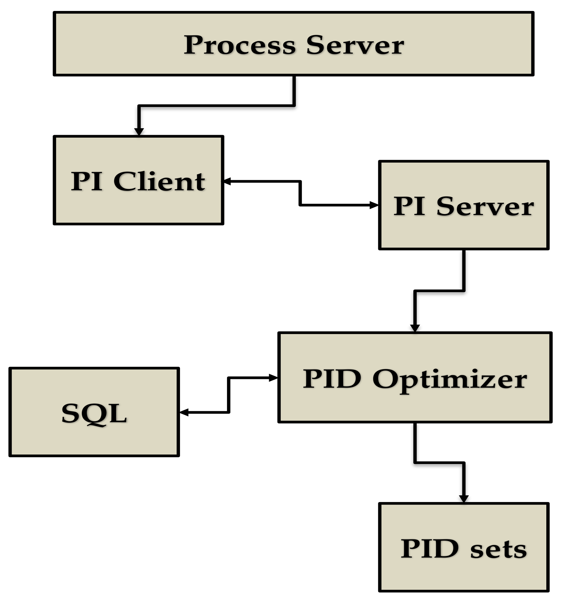
The operating system of the cooler is PCS7, Version 6.1, by Siemens AG (Munich, Germany). The software extracting data from the plant process server is PI, Version 3.2.0.0, by OSIsoft (San Leandro, CA, USA). The PI client acquires the process data with a sampling period of 5 s and stores them on the PI server. The data saved in this server constitute the plant database. The developed software, in C#, extracts from the PI server, using specific queries, specified data of the cooler with a 20 s period, and stores them in a Structured Query Language (SQL) database. Afterwards, it processes the SQL data, attempting to determine the optimal PID sets constituting a PID optimizer. Figure 2 presents a simplified diagram of this process.

Figure 2.
Data extraction and processing.
The main tasks of this optimizer are:
- Data extraction from PI and storing to SQL;
- Data extraction from SQL and determination of the best models;
- PID design;
- Simulation of the process to find the optimal PID gains.
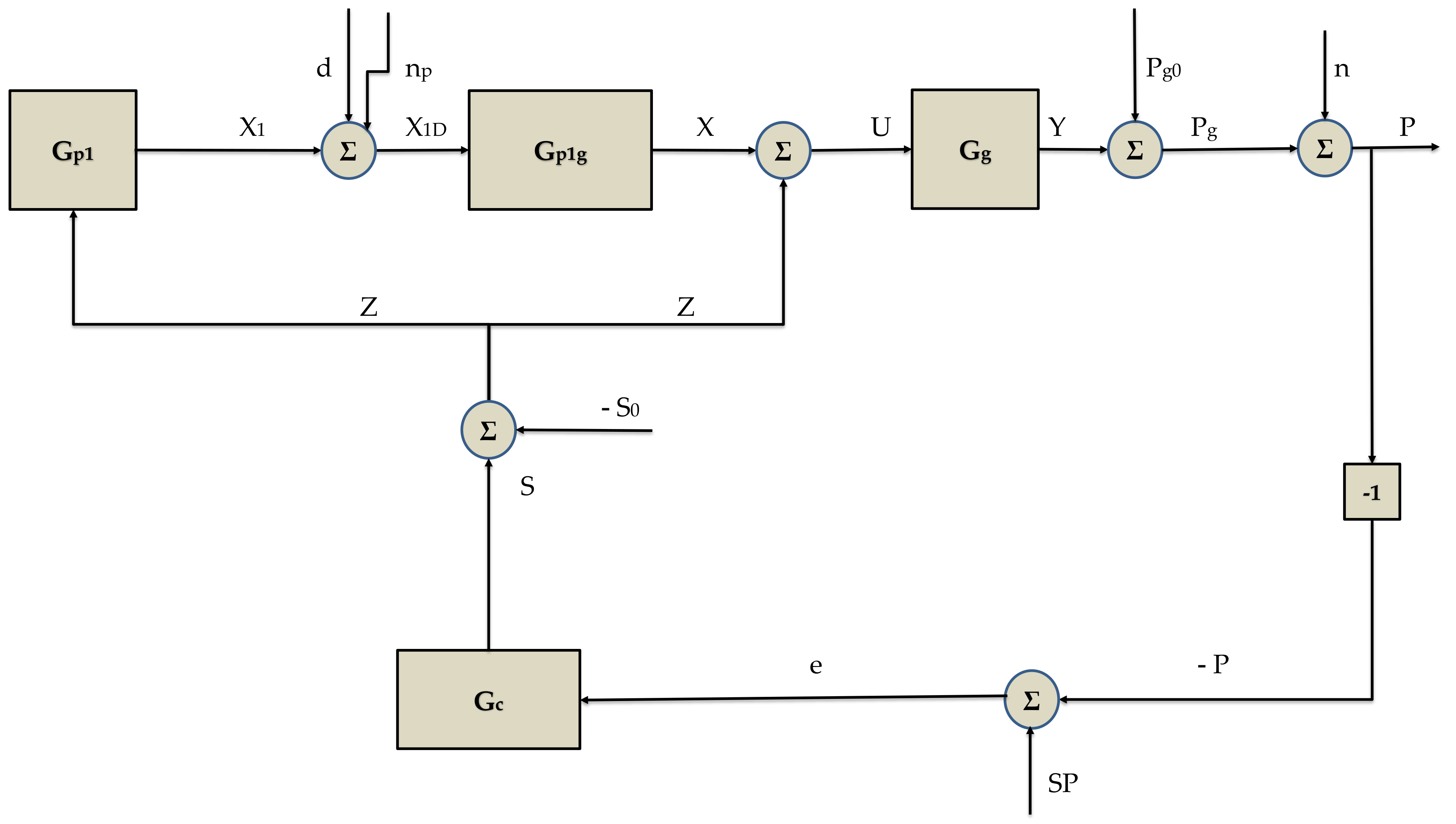
3. Process Model
The process model contains three transfer functions between the speed of the moving grate and the pressures of the static and moving grate, named Gp1, Gp1g, and Gg. The controller transfer function, Gc, is also included to realize the feedback control loop presented in Figure 3. All the signals are expressed as percentages.
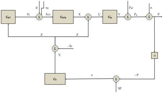
Figure 3.
Feedback control loop.
The transfer function between the speed of the grate, Z, and static grate output, X1, is given by the N-order Equation (1) in the Laplace domain.
where S is the speed of the moving grate and P1 represents the pressure of the fixed grate. The corresponding symbols of the steady state of the mentioned variables are S0 and P10, respectively. The dynamic parameters are the gain, kvp, the time constant, Tp, and the exponent, Np. A load disturbance, d, and noise, np, are added to X1, providing the input X1D to the second transfer function, Gp1g, as shown in Equation (2).
A first-order dynamic describes the transfer function between static and moving grates, according to Equation (3). The output of this function, X, if different from zero, constitutes a disturbance for the moving grate operation.
where the gain, kvpg, and the time constant, Tpg, are the dynamic parameters. The signals X and Z are summed up and inserted into the transfer function, Gg, of the moving grate, expressed by the N-order Equation (4).
where Pg is the pressure of the grate and Pg0 is the corresponding steady-state pressure for a speed equal to S0. U is the sum of the signals X and Z. The set of dynamic parameters consists of the gain, kvg, the time constant, Tg, and the exponent, Ng. The addition of the variable n, representing the noise, to the signal, Pg, derives the pressure, P. Equation (5) computes the control error which enters the controller transfer function, Gc, described by Equation (6).
The proportional, integral, and derivative gain of the PID controller are given by the set (kP, kI, and kD).
The sets of dynamic and steady-state parameters are the model parameters whose values need to be determined using actual process data. Process conditions and material characteristics affecting these parameters are:
- The flow rate and granulometry of clinker dropping from the kiln to the cooler;
- The flow rate, the number, and the quality of conventional and alternative fuels;
- The possible existence of rings inside the kiln;
- The pressures and probable clogging inside the preheater.
The variability of such conditions generates uncertainly as to parameters’ values. The parameters of each transfer function are estimated using the convolution theorem between the input signal, u, and the output variable, y, expressed by Equation (7).
where g(t) is the pulse system response. The following operating data were collected: (a) the speed, S, and pressure, P, of the first moving grate and (b) the pressure, P1, of the static grate. Appropriate software sampled these data. The optimal model parameters have been estimated by minimizing the residual error, sRes, using the Levenberg–Marquardt algorithm [23].
where M is the number of data in the defined period, k0 is the number of independent parameters, P(I) and P1(I) for I = 1 to M are the actual pressures of the moving and fixed grates, and PCalc(I) and P1,Calc(I) for I = 1 to M are the calculated pressures for the same period. The regression coefficient, RMod, is calculated by Equation (9).
where sP1 and sP are the standard deviations of the populations of P1 and P, respectively.
The sampling period corresponding to the time interval between two consecutive indices is Ts. At the time I, the errors between calculated and actual values are given by Equation (10) and represent both the signal noise and the modeling error. Autoregressive (AR) Equations (11) and (12) model both errors.
Equation (13) describe the same functions in the Laplace domain.
The disturbance, d, is modeled by a rectangular pulse of height, D0, and duration, TD.
4. Model Identification and Controller Design
4.1. Determining the Best Models
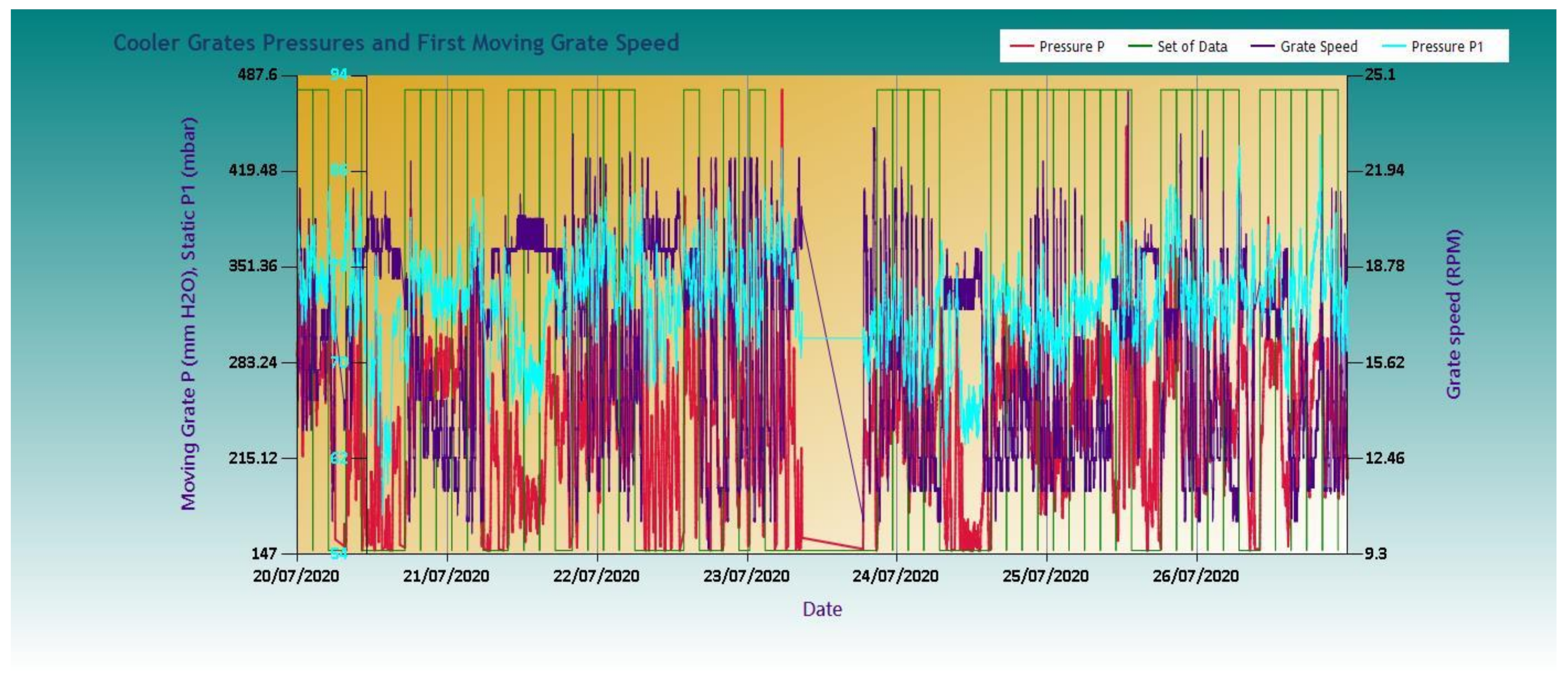
A module of the software is dedicated to loading and processing data of the cooler, directly extracted from the plant database with a sampling period, Ts, of 20 s. The selection of 20 s was made so that the sampling period is significantly shorter than the system time constants. The results should verify this decision. Along with the timestamp, the data of speed, pressure of the moving grate, and pressure of the fixed grate were extracted and then stored in an SQL database. Afterwards, the software downloads periods during which the kiln was operating from the database, removes the short downtime periods, and separates the remaining sets at 150-minute intervals. Table 1 shows the main characteristics of the cooler. Typical data sets, downloaded from the database and separated in 150-minute intervals, are demonstrated in Figure 4.

Table 1.
Cooler characteristics.

Figure 4.
Typical data sets extracted from the SQL database.
The following equations transform the process data into signals expressed as percentages:
where Sa is the speed of the first moving grate in RPM, P1a the pressure of the fixed grate in mbar, and Pa the pressure of the moving grate in mm H2O. Additionally, SaMin = 9.5 RPM, SaMax = 25 RPM, SMin = 33%, SMax = 55%, P1aMax = 100 mbar, and Pamax = 800 mm H2O.
A wide variety of models described by Equations (1), (3) and (4) were studied, selecting an extended range of exponents, Np and Ng. Np took all integer values in the interval (1, 9), while Ng took the integer values in the interval (2, 9). Equations (17) and (18) calculate the residual errors for each experimental data series. For every period of 150 min, the software utilizes the results of the first 30 min to build the initial values by convolution, while those of the last 120 min were used to compare experimental and calculated pressures. Therefore, for Ts = 20 s, M = 360. Equations (19) and (20) give the corresponding regression coefficients.
For each data set of 150-minute duration, the algorithm finds the optimal dynamic parameters first by minimizing the sRes and then calculates the other two residual errors and the regression coefficients. For some values of Np and Ng, the parameters needing determination are (a) the gains, kvp, kvpg, and kvg; (b) the time constant, Tp, Tpg, and Tg; and (c) the steady-state values, S0, P10, and Pg0, resulting in k0 = 9. The parameters kvp, Tp, S0, and P10 are entered into Equation (17), thus k1 = 4, while kvpg, kvg, Tpg, Tg, S0, and Pg0 are included in Equation (18), therefore k2 = 6. The processed data sets of 150-minute duration amounted to 949, resulting in approximately 450,000 groups of data. The validity of the modeling is assessed by comparing the achieved regression coefficients. The percentages of the data sets with regression coefficients, according to Equations (9), (19) and (20), higher than certain thresholds are presented in Table 2, Table 3 and Table 4.
Table 2.
Percentages of data sets with RMod ≥ 0.7.
Table 3.
Percentages of data sets with RP1 ≥ 0.7.
Table 4.
Percentages of data sets with RP ≥ 0.8.
The results of these three tables lead to the following conclusions:
- As far as the model regression coefficient is concerned, RMod, for 4 ≤ Ng ≤ 7 and 4 ≤ Np ≤ 9, more than 77% of the data sets present a RMod ≥ 0.7.
- The regression coefficient, RP, between P, P1, and S is higher than 0.8 for more than 67% of the data sets if Ng ≥ 4.
- As to the corresponding regression coefficient between P1 and S, there exist enough combinations of (Np, Ng) pairs where more than 42% of the total sets have a RP1 ≥ 0.7.
- RP1 is generally less than RP due to the load disturbances coming from the kiln side.
- The modeling verifies the measurable impact of the speed of the moving grate on the pressure of the static grate.
The determination of a suboptimum area in the plane (Np, Ng) is done as follows: in Table 3, suboptimal pairs (Np, Ng) are those where the percent is higher than 90% of the maximum value. Respectively, in Table 4, the pairs (Np, Ng) are defined as those with percentages higher than 95% of the highest value. The section of both regions, shown with the symbol “X” in the cells of Table 5, provides the area of exponents satisfying both suboptimal conditions.
Table 5.
Exponents of optimal models.
After selecting the data sets with a RMod ≥ 0.7, the mean values and standard deviations of the dynamic and steady-state parameters for (Np, Ng) = (6, 6) and (Np, Ng) = (4, 4) were calculated and are shown in Table 6. The variance in the dynamic parameters is very high, probably causing problems in a robust automatic control strategy. As the exponents of the models increase, the three constants, Tp, Tpg and Tg, decrease. The total time lag depends not only on the time constants but also on the exponent of the dynamics. For each set of exponents, the non-linear regression technique tries to find the time constants so that the adjustment of experimental and calculated values is optimal. The mean time constants are from 4.5 min to 6 min, 13 to 18 times bigger than the sampling period of 20 s. Therefore, the selection of this period is correct.
Table 6.
Dynamic and steady-state parameters.
Figure 5a,b depicts the experimental and calculated results for two models. These figures are part of the user-friendly interface provided by the software. One can observe that the fitting of calculated results to the actual ones is better for the moving grate than for the fixed, regardless of the model. The reason is that the pressure, P1, is affected not only by the speed, S, but also by disturbances arriving from the kiln.
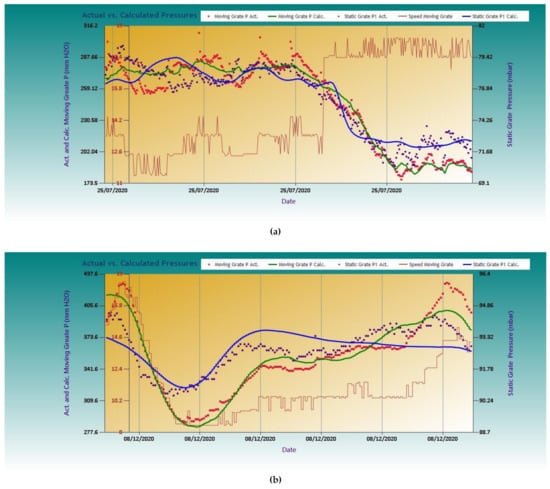
Figure 5.
Calculated vs. actual values for the models: (a) Np = 6, Ng = 6; (b) Np = 4, Ng = 4.
4.2. PID Controller Design
Guaranteeing robustness is a central theme in modern control theory. During the design and parameterization of the controller, when severe load disturbances or high uncertainty in the model parameters occur, the designer must ensure the stability and efficiency of the loop. A technique for adjusting PID controllers is the robust loop-shaping method [24,25]. Such an effective loop-shaping technique is the MIGO (M-constrained integral gain optimization) method, developed by Astrom, Panagopoulos, and Hagglund [2,3,16,26]. Tsamatsoulis successfully applied this method in other cases of automatic control of cement production processes [17,18,20,21,22]. The approach is to maximize the integral gain for a certain value of the maximum sensitivity, Ms, defined by Equations (21) and (22). The letter “M” in the MIGO method comes from the maximum sensitivity constraint.
where S is the sensitivity as a function of the frequency, ω, and GL the open-loop transfer function, given by Equation (23). This transfer function is calculated by interrupting the signal of pressure, P, before adding it to the set-point, SP, and opening the loop.
Among the models shown in Table 5, the model with Np = 6 and Ng = 6 was chosen because it is close to the middle of the region. Then, for Ms belonging to the interval of 1.1 to 1.7, and with a stepwise increase of 0.1, the sets (kP, kI, and kD) are computed. The two independent variables are the set (Ms, kD) and the method that calculates the set (kP, kI), satisfying the robustness constraint. The algorithm is given in [2] (pp. 206–221) and an analytical implementation in [17].
The Nyquist curve of a system is the locus of the complex number, GL(iω), as ω goes from 0 to ∞ [2] (p. 22). Figure 6 shows the Nyquist curve of the GL function for (kP, kI, and kD) = (0.6922, 0.0305, and 1), corresponding to Ms = 1.3. From this figure, the method becomes obvious: the algorithm for given values of Ms, kD finds values of kP, kI, if such values exist, so that the curve GL is tangent to a circle, centered at the point (−1, 0) and with a radius of 1/Ms. Figure 7 demonstrates the functions between kP, kI, and Ms, kD.
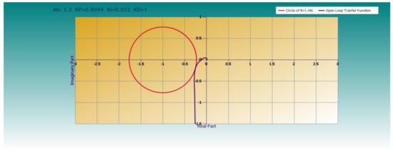
Figure 6.
Nyquist curve of the open-loop transfer function for Ms = 1.3 and kD = 1.
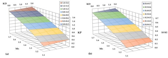
Figure 7.
Function between (a) kP and Ms, kD; (b) kI and Ms, kD.
4.3. Autoregressive Model
The algorithm checked the adequacy of the autoregressive model for ErrP and ErrP1 errors for the dynamic models with (Np, Ng) = (6, 6) and (Np, Ng) = (4, 4). Table 7 presents (a) the coefficients; (b) average standard errors; (c) regression coefficients, R, of Equations (11) and (12); and (d) the values of sResP1, sResP.
Table 7.
Autoregressive model parameters.
One can conclude the following from these results: (a) the regression coefficients of both autocorrelation models are sufficiently high, implying that the errors sResP1 and sResP represent a colored noise; (b) the coefficients are very similar for both dynamic models; and (c) the sum of the two coefficients has a significantly smaller standard deviation than each coefficient separately, meaning that one can consider this sum as constant.
5. PID Optimization by Simulation
The control variable affects not only the process variable but also a variable that is a process disturbance, making, for this reason, the control loop shown in Figure 3 particularly interesting. In addition, high uncertainty characterizes the dynamics. Therefore, to find the optimal PID coefficients, a simulation is required that considers as many process characteristics as possible. The optimization criterion is the integral of absolute error between P and SP, as a percentage of SP defined by Equation (24). The integration time is an interval, t0. IAE is an acceptable criterion of optimization because a sluggish or much faster controller would give higher errors compared to a robust controller, especially in the presence of load disturbances.
The simulator can select the PID sets found by the MIGO technique in Section 4.2 and simulates the cooler for each (kp, ki, and kd). Equation (25) provides the digital form of PID implementation.
where Ts is the sampling and actuator period in seconds, e(I), e(I − 1), and e(I − 2) are the errors, e, given by Equation (5) in time domain, at the moments I, I − 1, and I − 2, respectively, and Sold and Snew are the previous and the new speed, respectively. The operating system of the cooler uses the same digital form. The simulator settings are the following:
- (i)
- The setpoint of pressure, Pa, of moving grate, SPa;
- (ii)
- The current minimum value of speed, Scmin;
- (iii)
- The values of dynamic and steady-state parameters of the transfer functions (1), (3) and (4);
- (iv)
- Percent disturbance margin for each of the nine dynamic and steady-state parameters;
- (v)
- The values of coefficients, A1P and A2P, and of standard error, StdErrP, of Equation (11);
- (vi)
- The values of coefficients, A1P1 and A2P1, and of standard error, StdErrP1, of Equation (12);
- (vii)
- The values of residual errors, sResP1 and sResP, according to Equations (17) and (18);
- (viii)
- The sampling and actuator period, Ts;
- (ix)
- The total time of simulation, Toper;
- (x)
- The minimum and maximum number of sampling periods during which the load disturbance is present;
- (xi)
- The total number of simulations per software module execution, NI.
5.1. Short Description of the Simulator
The simulator uses the dynamic model with (Np, Ng) = (4, 4), which belongs to the optimal models’ area and shows the lowest residence time compared to other models due to its lower exponents. According to Astrom [2] (pp. 25, 33), the average residence time of an N-order model with a time constant, T0, is N·T0. The simulation uses the median values of dynamic parameters as reference values. The steady-state parameters are not independent of each other: when S0 increases, both P10 and Pg0 decrease. After grouping the steady-state parameters of the model with (Np, Ng) = (4, 4) and a RMod ≥ 0.7, linear expressions, described by Equations (26) and (27), were extracted.
Table 8 presents the values of the three steady-state parameters for several pressures, Pa, in mm H2O, according to Equations (16), (26) and (27).
Table 8.
Values of steady-state parameters.
The objective of the simulator is to find the PID sets, among those shown in Figure 7, which achieve the minimum IAE by performing both set-point tracking and load disturbance attenuation. The simulator starts at a moving grate speed and pressures equal to steady-state values so that the movable grate pressure is 75 mm H2O below the set-point. Table 9 shows the data used. The total operating time of the simulator is 360 min. During the first 30 min, the simulator performs the initial convolutions between input signals and frequency responses, and then each new point is calculated from the last 1800/Ts points. The cooler runs in manual mode during these first 30 min with constant grate speed and then runs in automatic mode. A random white noise belonging to the interval (−sResP, sResP) is added to the first two points, P, while for the following pressures, P, the noise is added according to Equation (11). The same procedure is followed for the pressure, P1, using the residual error, sResP1, and Equation (12). Disturbance, D, lasts from Tdist,min to Tdist,max minutes, and its amplitude is a random number belonging to the interval (−MP10/100·P10, MP10/100·P10). The disturbance enters the system halfway through the operating time. The simulator every Ts seconds provides the new speed based on Equation (25). In each of the NI simulations, the parameters change randomly around the reference values, within a range ± ma/100, where ma is the maximum disturbance margin. The value of the ma of each parameter is given in rows 8–11, 14–15, and 20–22 of Table 9. There is also a minimum grate speed, SLow, to prevent the grate from completely stopping when the thickness of the bed is too small.
Table 9.
Simulator settings.
The simulator calculates IAE in each run, then the average IAENI for all NI runs. Because the count of uncertainties is large and their magnitude is significant, a criterion for IAE convergence is required. If the simulator runs K times and NI times in each run, then the average IAE(K) is:
Then if in the next K + 1 iteration satisfies condition (29), IAE is converged to IAEAver. If not, further iterations are needed.
5.2. Initial Simulations
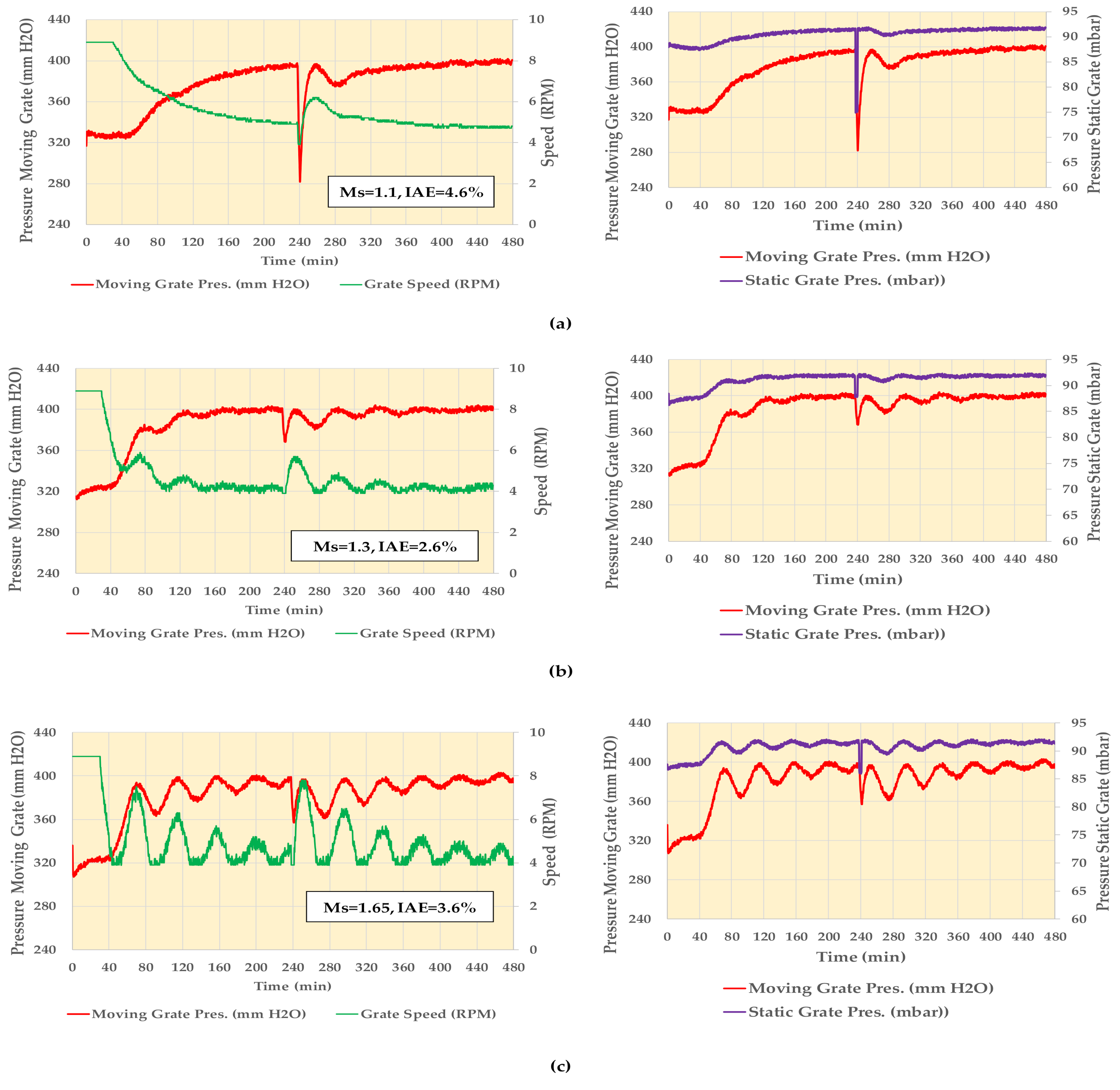
Before implementing the simulator, by using the full range of PID sets and parameter uncertainty, some preliminary simulations were performed to investigate the impact of maximum sensitivity function, Ms, on the performance and robustness of the control.
The simulator executed three times with SPa = 400 mm H2O, NI = 1, total simulation time equal to 480 min, and the following controller parameters:
- Ms = 1.1, kP = 0.289, kI = 0.011, kD = 0.0;
- Ms = 1.3, kP = 0.78, kI = 0.031, kD = 0.5;
- Ms = 1.65, kP = 1.348, kI = 0.056, kD = 0.0.
For the initial simulations, the selection of a run time higher than that of Table 9 is necessary for checking the behavior of the controllers in a better manner in a longer operating time. Figure 8 depicts the controller’s action with the different settings in set-point tracking and attenuating the load disturbances. All controllers stabilize the process, but each has its characteristics. One can observe the following in Figure 8a. The velocity of reaching the set-point is very slow with the low Ms controller. In particular, if the load disturbance results in a reduction of the static grate pressure, then it is hard for the controller to approach the set-point within a reasonable time. Such a disturbance occurs when the operator reduces the kiln speed to keep the material in the kiln. The response of the controller with the highest Ms, in Figure 8c, has oscillations, and if the load disturbance is in the same direction as the rate of change of the moving grate pressure, the amplitude of the oscillations increases. The controller with Ms = 1.3, in Figure 8b, is the more robust one: it reaches the set-point within a reasonable time and reacts with rapidly damped oscillation to an intense load disturbance.

Figure 8.
Function between pressure of moving grate, grate speed, and pressure of static grate for (a) Ms = 1.1, kD = 0; (b) Ms = 1.3, kD = 0.5; and (c) Ms = 1.65, kD = 0.
5.3. Full Simulation and PID Optimization
The simulation applies all the PID sets calculated in Section 4.2 to the process data and the uncertainty margins shown in Table 9. The required number of iterations to fulfill condition (19) is 5·NI = 1000. Figure 9 shows the values of IAEAver as a function of Ms and kD for SPa = 400 mm H2O.
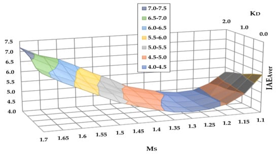
Figure 9.
IAEAver as a function of Ms, kD for SPa = 400 mm H2O.
The calculations for determining the PID area, which presents the best IAEAver, are the following:
- (a)
- The PID set providing the minimum IAEAver,Min was found;
- (b)
- The sets with IAEAver ≤ 1.1·IAEAver,Min were determined;
- (c)
- This area constitutes the optimum region of the PID coefficients.
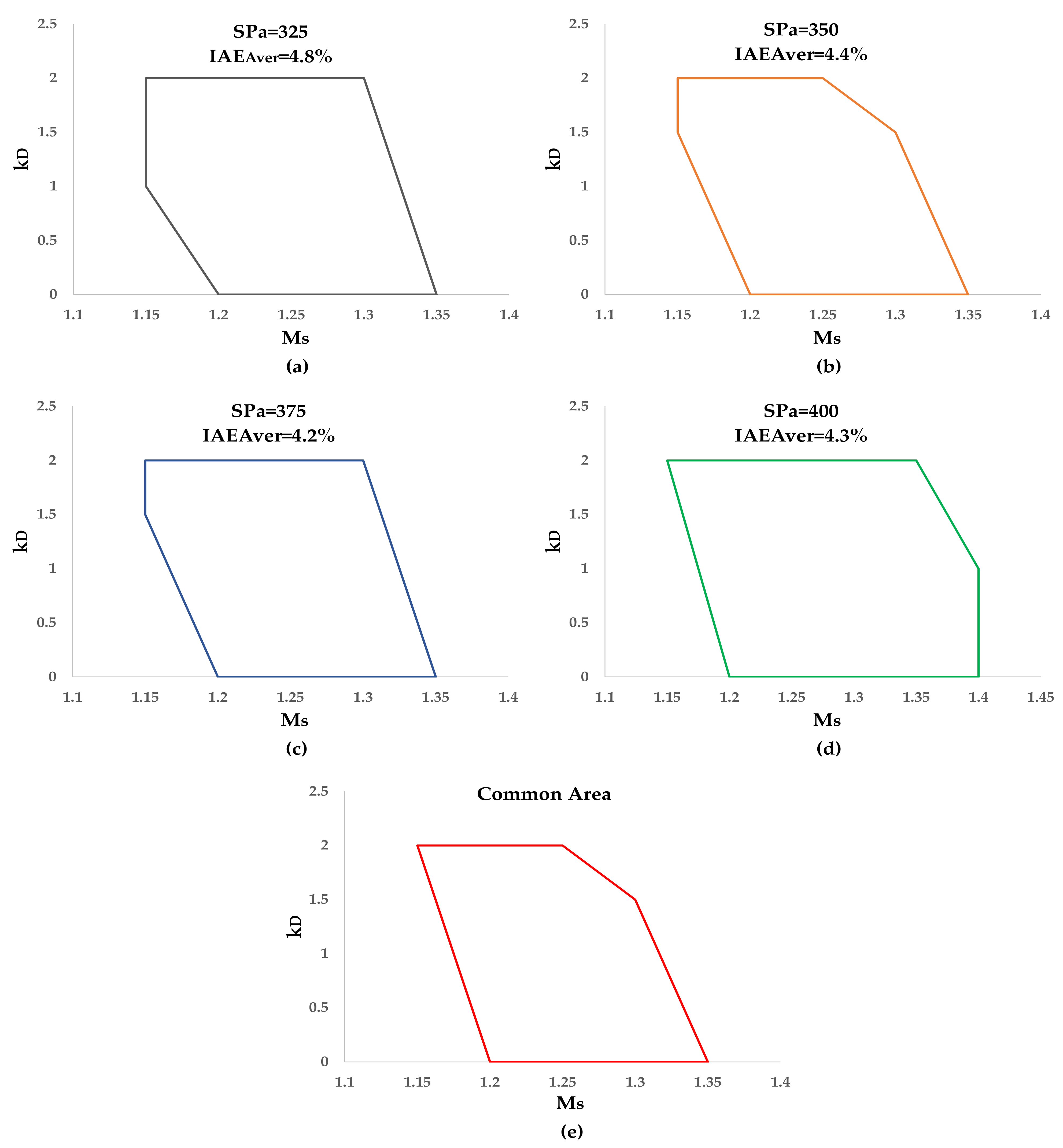
Figure 10 depicts the optimal region of PID controllers per set-point as well as the common area. The values of IAEAver,Min per set-point also appear in this figure.
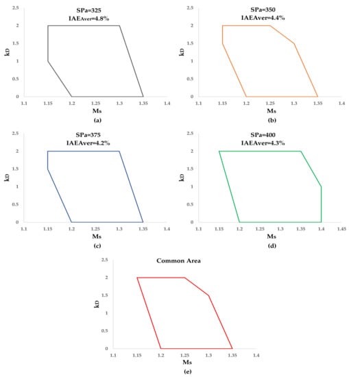
Figure 10.
Optimal PID controllers for SPa: (a) 325 mm H2O; (b) 350 mm H2O; (c) 375 mm H2O; (d) 400 mm H2O; and (e) common area of all SPa.
In conclusion, the combination of a robustness constraint with a performance criterion, maximum sensitivity, and integral of absolute error, respectively, leads to determining an optimal area of PID coefficients. PID sets located near the middle of this area can be chosen and implemented in the routine operation of the cooler under examination.
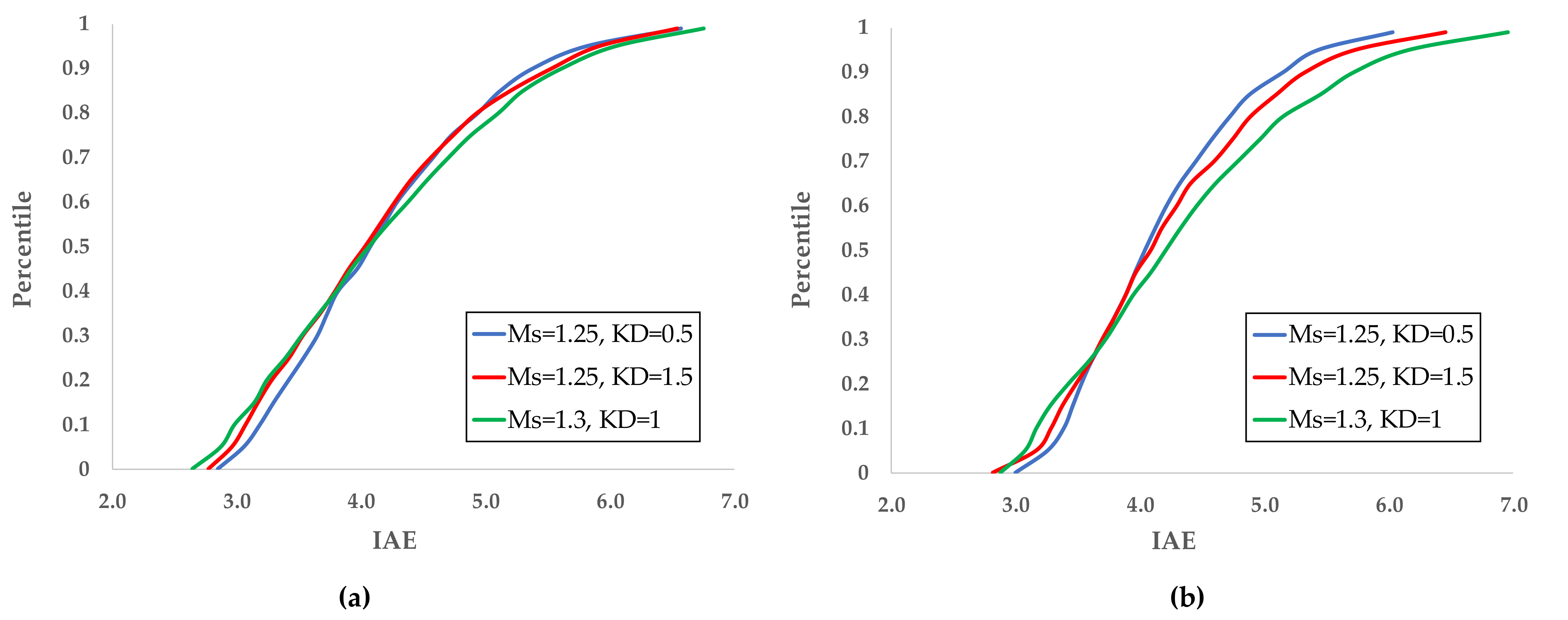
The study of the distribution of IAE for PIDs belonging to the optimal region was performed by applying the simulation for NI = 1000 and three sets (kP, kI, and kD) with values shown in Table 10. Figure 11a,b demonstrates the percentiles of IAE for SPa = 400 mm H2O and SPa = 375 mm H2O, respectively.
Table 10.
PID sets for studying IAE distribution.
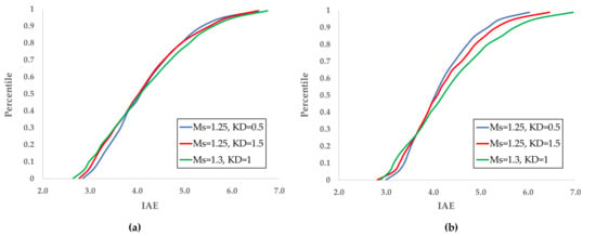
Figure 11.
IAE distributions for SPa: (a) 400 mm H2O; (b) 375 mm H2O.
For SPa = 400 mm H2O, the three controllers are almost equivalent: the median IAE is ~4%, while 80% of IAEs are less than ~5%. On the other hand, for SPa = 375 mm H2O, the performance differences of the three controllers are not negligible: the smaller IAEs occur with the slow controller, with Ms = 1.2 and kD = 0.5, and the differences become more significant for higher percentiles. Therefore, a weak impact of the set-point value on the optimal PID gains exists.
6. Conclusions
By implementing dynamic models of clinker cooling, efficient efforts have been made in optimizing the PID controller regulating the process. The modeling utilizes exclusively industrial data of the cooler of the Halyps cement plant. The process model contains three transfer functions between the speed of the moving grate and the pressures of the static and moving grate. The two transfer functions between the speed and the two pressures are expressed by N-order dynamics, while the third between the pressures of fixed and moving grate is expressed by first-order dynamics. The models include dynamic parameters such as gains and time constants, steady-state variables, and exponents of the dynamics. The best models’ identification was achieved by implementing non-linear regression methods. The process model uses high-efficiency autoregressive equations to express the signal’s noise and model mismatch and a rectangular pulse to describe the load disturbances.
Based on modeling results, the design of the PID controller follows according to a loop-shaping technique, which considers as a constraint the maximum sensitivity, Ms, of the open-loop transfer function. The output of this algorithm is a set of PIDs satisfying a range of Ms constraints. The control variable affects not only the process variable but also a variable that is a process disturbance, making, for this reason, the control loop particularly interesting. A simulator determines the optimal PID sets, among those calculated at the design step, using the IAE as a performance criterion, where a table of 35 inputs constitutes the simulator’s settings. The combination of a robustness constraint with a performance criterion, maximum sensitivity, and integral of absolute error, respectively, leads to controllers with Ms belonging to the range of 1.2 to 1.35. The IAE is between 4.2% and 4.8%, depending on the set-point value. These results are a strong argument that the cooler investigated can be effectively regulated by the designed PID.
Funding
This research received no external funding.
Institutional Review Board Statement
Not applicable.
Informed Consent Statement
Not applicable.
Data Availability Statement
Not applicable.
Conflicts of Interest
The authors declare no conflict of interest.
Nomenclature
| A1P, A2P | Coefficients of the autoregressive Equation (11) |
| A1P1, A2P1 | Coefficients of the autoregressive Equation (12) |
| d | Pressure load disturbance on the fixed grate, % |
| D0 | Maximum height of the disturbance, d, % |
| e | Control error between SP and P, % |
| ErrP | Error between P and PCalc |
| ErrP1 | Error between P1 and P1,Calc |
| IAE | Integral of absolute error, % |
| k0 | Number of independent variables in Equation (8) |
| kD | Derivative gain of the PID controller, min |
| kI | Integral gain of the PID controller, min−1 |
| kP | Proportional gain of the PID controller |
| kvp | Gain of the transfer function Gp1 |
| kvpg | Gain of the transfer function Gp1g |
| kvg | Gain of the transfer function Gg |
| Gc | Transfer function of the PID controller |
| Gg | Transfer function between moving grate speed and pressure of moving grate |
| GL | Open-loop transfer function |
| Gp1 | Transfer function between moving grate speed and pressure of static grate |
| Gp1g | Transfer function between pressures of static and moving grate |
| M | Count of data in the defined period |
| Ms | Maximum sensitivity |
| NI | Number of simulations |
| Np | Exponent of the function Gp1 |
| np | Pressure noise on the fixed grate, % |
| Ng | Exponent of the function Gg |
| ng | Pressure noise on the moving grate, % |
| P | Pressure of moving grate after the addition of the noise, n, % |
| Pa | Pressure of moving grate, mm H2O |
| PaMax | Maximum pressure of moving grate, mm H2O |
| P1a | Pressure of static grate, mbar |
| P1aMax | Maximum pressure of static grate, mm H2O |
| PCalc | Calculated pressure of moving grate, % |
| Pg | Pressure of moving grate, % |
| P1 | Pressure of static grate, % |
| P1,Calc | Calculated pressure of static grate, % |
| P10 | Steady-state pressure of static grate, % |
| Pg | Pressure of moving grate, % |
| Pg0 | Steady-state pressure of moving grate, % |
| RMod | Model regression coefficient for pressures P and P1 |
| RP | Regression coefficient between pressures P and PCalc |
| RP1 | Regression coefficient between pressures P1 and P1,Calc |
| S(iω) | Sensitivity function |
| S | Moving grate speed, % |
| Sa | Moving grate speed, RPM |
| SaMax | Maximum speed, Sa, RPM |
| SaMin | Minimum speed, Sa, RPM |
| SMax | Maximum speed, S, % |
| SMin | Minimum speed, S, % |
| S0 | Steady-state speed of moving grate, % |
| SLow | Low limit of grate speed, % |
| sP | Standard deviation of the population of pressures, P, % |
| SP | Set-point of pressure in moving grate, % |
| SPa | Set-point of pressure in moving grate, RPM |
| sP1 | Standard deviation of the population of pressures, P1, % |
| sRes | Residual error between actual and calculated pressures, % |
| sResP | Residual error between pressures P and PCalc, % |
| sResP1 | Residual error between pressures P1 and P1,Calc, % |
| StdErrP | Standard error of the Equation (11), % |
| StdErrP1 | Standard error of the Equation (12), % |
| t0 | Integration time in Equation (24), min |
| tD | Duration of the disturbance, d, min |
| Tp | Time constant of the transfer function Gp1, min |
| Tpg | Time constant of the transfer function Gp1g, min |
| Ts | Sampling and actuation period, s |
| Tg | Time constant of the transfer function Gg, min |
| U | Sum of the signals X and Z, % |
| Χ | Output pressure from the transfer function Gp1g, % |
| X1 | Difference between P1 and P10, % |
| Y | Difference between Pg and Pg0, % |
| X1D | Sum of the signals X1, d, and np, % |
| Z | Difference between S and S0, % |
References
- Miglay, H.G. The formation and phase composition of portland cement clinker. In The Chemistry of Cements, 2nd ed.; Taylor, H.F.W., Ed.; Academic Press Inc.: New York, NY, USA, 1972; Volume 1, pp. 103–106. [Google Scholar]
- Astrom, K.J.; Hagglund, T. Advanced PID Control; Instrumentation, Systems and Automatic Society: Raleigh, NC, USA, 2006; pp. 1, 25, 33, 206–221. [Google Scholar]
- Astrom, K.J. Model Uncertainty and Robust Control, Lecture Notes on Iterative Identification and Control Design, Lund University. 2000. Available online: https://www.researchgate.net/publication/228602986_Model_Uncertainty_and_Robust_Control/ (accessed on 1 July 2021).
- Tsamatsoulis, D. Simplified Modeling of Clinker Cooling Based on Long Term Industrial Data. In Proceedings of the Recent Researches in System Science, 15th WSEAS International Conference on Systems, Corfu Island, Greece, 14–16 July 2011; WSEAS Press: Stevens Point, WI, USA, 2011; pp. 143–147. Available online: http://www.wseas.us/e-library/conferences/2011/Corfu/SYSTEMS/SYSTEMS-21.pdf (accessed on 1 July 2021).
- Srividhya, G.; Guruprasath, M.; Jayalalitha, S. Maintenance of under Grate Pressure in Grate Coolers Used in Cement Kilns by IMC Based PID Controller. Int. J. Adv. Res. Electr. Electron. Instrum. Eng. 2015, 4, 1692–1699. Available online: http://www.ijareeie.com/upload/2015/march/63_MAINTENANCE_new.pdf (accessed on 1 July 2021).
- Yu, H.; Sun, Y.; Huang, B.; Zheng, Z. Research on Modelling of Grate Cooler Based on Typical Operating Conditions. In Proceedings of the 2nd International Conference on Intelligent Manufacturing and Materials—Volume 1, Guangzhou, China, 15–16 June 2018; Sup, K., Ed.; pp. 556–561. Available online: https://www.scitepress.org/Papers/2018/75356/75356.pdf/ (accessed on 11 June 2021).
- Wang, X.; Wu, S.; Shen, T.; Fan, Y. The Grey Predictive Control on Grate Cooler System. In Proceedings of the 2007 Chinese Control Conference, Zhangjiajie, China, 26–31 July 2007; pp. 218–221. Available online: https://ieeexplore.ieee.org/document/4347202 (accessed on 1 July 2021).
- Jun, Z.M.; Qingjin, M.; Hongliang, Y. The Application of Dynamic Matrix Control in the Grate Cooler. In Proceedings of the 2017 IEEE 2nd Advanced Information Technology, Electronic and Automation Control Conference, Chongqing, China, 25–26 March 2017; pp. 2630–2633. Available online: https://ieeexplore.ieee.org/document/8054501 (accessed on 1 July 2021).
- Wang, Z.; Yuan, M. A Self-Tuning Fuzzy PID Control Method of Grate Cooler Pressure Based on Kalman Filter. In Proceedings of the 2012 International Conference on Computer Science and Information Processing, Xi’an,China, 24–26 August 2012; Available online: http://www.greenid.ir/wpimages/13GREENID%20A%20Self-tuning%20Fuzzy%20PID%20Control%20Method.pdf/ (accessed on 12 June 2021).
- Zhang, X.; Lu, J. Fuzzy Control of Heat Recovery Systems of Cement Clinker Cooler. J. Theor. Appl. Inf. Technol. 2012, 4, 182–190. Available online: http://www.jatit.org/volumes/Vol42No2/5Vol42No2.pdf (accessed on 1 July 2021).
- Karikov, E.B.; Rubanov, V.G.; Korneevich, K.V. Construction of a Dynamic Neural Network Model as a Stage of Grate Cooler Automation. World Appl. Sci. J. 2013, 25, 227–232. Available online: https://www.idosi.org/wasj/wasj25(2)13/9.pdf (accessed on 1 July 2021).
- Elman, J.L. Finding Structure in Time. Cogn. Sci. 1990, 14, 179–211. [Google Scholar] [CrossRef]
- Seraj, M.; Shooredeli, M.A. Data-Driven Predictor and Soft-Sensor Models of a Cement Grate Cooler Based on Neural Network and Effective Dynamics. In Proceedings of the 2017 Iranian Conference on Electrical Engineering, Tehran, Iran, 2–4 May 2017; pp. 726–731. Available online: https://ieeexplore.ieee.org/document/7985134 (accessed on 1 July 2021).
- Geng, Y.; Wang, X.; Jiang, P. Prediction of the Cement Grate Cooler Pressure in the Cooling Process Based on a Multi-Model Fusion Neural Network. IEEE Access 2020, 8, 115028–115040. Available online: https://ieeexplore.ieee.org/document/9118923 (accessed on 1 July 2021). [CrossRef]
- Wang, S.; Yu, H.; Lu, S.; Wang, X.; Liu, H. Application of Least Square Support Vector Machine with Adaptive Particle Swarm Parameter Optimization in Grate Pressure Optimization Setting of Grate Cooler. In Proceedings of the 2020 35th Youth Academic Annual Conference of Chinese Association of Automation, Zhanjiang, China, 16–18 October 2020; pp. 632–637. Available online: https://ieeexplore.ieee.org/document/9337619 (accessed on 1 July 2021).
- Astrom, K.J.; Panagopoulos, H.; Hagglund, T. Design of PI Controllers Based on Non-Convex Optimization. Automatica 1998, 34, 585–601. [Google Scholar] [CrossRef]
- Tsamatsoulis, D. Effective Optimization of the Control System for the Cement Raw Meal Mixing Process: I. PID Tuning Based on Loop Shaping. WSEAS Trans. Syst. Control 2011, 6, 239–253. Available online: http://www.wseas.us/e-library/transactions/control/2011/52-480.pdf (accessed on 13 June 2021).
- Tsamatsoulis, D. Effective Optimization of the Control System for the Cement Raw Meal Mixing Process: II. Optimizing Robust PID Controllers Using Real Process Simulators. WSEAS Trans. Syst. Control 2011, 6, 276–288. Available online: http://wseas.us/e-library/transactions/control/2011/52-697.pdf (accessed on 13 June 2021).
- Tsamatsoulis, D. Modelling and simulation of raw material blending process in cement raw mix milling installations. Can. J. Chem. Eng. 2014, 92, 1882–1894. [Google Scholar] [CrossRef]
- Tsamatsoulis, D. Dynamic Behavior of Closed Grinding Systems and Effective PID Parameterization. WSEAS Trans. Syst. Control 2009, 4, 581–602. Available online: http://www.wseas.us/e-library/transactions/control/2009/29-816.pdf (accessed on 13 June 2021).
- Tsamatsoulis, D. Optimizing the control system of cement milling: Process modeling and controller tuning based on loop shaping procedures and process simulations. Braz. J. Chem. Eng. 2014, 31, 155–170. [Google Scholar] [CrossRef]
- Tsamatsoulis, D.; Zlatev, G. PID Parameterization of Cement Kiln Precalciner Based on Simplified Modeling. Available online: https://www.naun.org/main/NAUN/neural/2016/a142016-083.pdf (accessed on 14 June 2021).
- Marquardt, D.W. An Algorithm for Least-Squares Estimation of Nonlinear Parameters. SIAM J. Appl. Math. 1963, 11, 431–441. [Google Scholar] [CrossRef]
- Zolotas, A.C.; Halikias, G.D. Optimal Design of PID Controllers Using the QFT Method. IEE Proc. Control Theory Appl. 1999, 146, 585–590. Available online: https://digital-library.theiet.org/content/journals/10.1049/ip-cta_19990746 (accessed on 1 July 2021). [CrossRef] [Green Version]
- Yaniv, O.; Nagurka, M. Automatic Loop Shaping of Structured Controllers Satisfying QFT Performance. J. Dyn. Syst. Meas. Control 2005, 127, 472–477. Available online: https://www.researchgate.net/publication/229003095_Automatic_Loop_Shaping_of_Structured_Controllers_Satisfying_QFT_Performance (accessed on 1 July 2021). [CrossRef] [Green Version]
- Astrom, K.J.; Hagglund, T. Revisiting the Ziegler–Nichols step response method for PID control. J. Process. Control 2004, 14, 635–650. [Google Scholar] [CrossRef]


Publisher’s Note: MDPI stays neutral with regard to jurisdictional claims in published maps and institutional affiliations. |
© 2021 by the author. Licensee MDPI, Basel, Switzerland. This article is an open access article distributed under the terms and conditions of the Creative Commons Attribution (CC BY) license (https://creativecommons.org/licenses/by/4.0/).