Three-Dimensional CFD Model Development and Validation for Once-Through Steam Generator (OTSG): Coupling Combustion, Heat Transfer and Steam Generation

Abstract

The current research studies the coupled combustion inside the furnace and the steam generation inside the radiant and convection tubes through a typical Once-Through Steam Generator (OTSG). A 3-D CFD model coupling the combustion and the two-phase flow was developed to model the entire system of OTSG. Once the combustion simulation was converged, the results were compared to field data showing a convincing agreement. The CFD analysis provides the detailed flow behavior inside the combustion chamber and the stack, as well as the two-phase flow steam generation process in the radiant and convective sections. The flame shape and orientation, the velocity, the species, and the temperature distribution at the various parts of the furnace, as well as the steam generation and the steam distribution inside the pipes were investigated using the developed CFD model

1. Introduction

The oil extraction industry in northern Alberta relies on the use of large Once-Through Steam Generators (OTSGs). Efficient steam generation with as low as possible pollutant emissions is a high priority for economic and environmental reasons. The OTSGs are commonly used in Steam-Assisted Gravity Drainage (SAGD) operations which is an advanced oil recovery technology for heavy crude oil and bitumen production. There are several reasons for using OTSGs instead of conventional steam drum type boiler for this type of application, the two main reasons being the elimination of steam drum which reduces the maintenance cost, and lowers corrosion rate at the tubes inner surface.

Generally speaking, OTSGs are usually composed of three main parts: the burner, the radiant section, and the convective section. Natural gas is burned through staged diffusive flames stabilized by the burner. The heat generated by the combustion is transferred to the water flowing through the piping system in the radiant and convective sections. The steam produced within the pipes is then injected underground to reduce the oil viscosity and allow its pumping to the surface.

Until now, the design and operation of large OTSGs have been relying on somewhat simplified models and calculations heavily backed by experience developed over the years on evolving design of increasing size and complexity, in our opinion, this approach has reached its limits. The availability of powerful numerical simulation techniques will certainly be of benefit to the field, as it has been proved in other industries (Charles and Baukal [1]). The progress towards increasing efficiency and reliability of the equipment can be achieved only through the use of more advanced numerical simulations (Charles and Baukal [1]).

Simulation and computer assisted engineering services are not sufficiently developed to satisfy the current needs of producers. Improvements in the modeling methodologies to make them faster, more reliable, and efficient for solving large problems are necessary to encourage the producers to adopt and deploy these tools widely. The development of such tools and approaches gives a competitive advantage in the marketplace and will help producers meet production; financial; and health, safety, environmental (HSE) goals in a more stringently regulated industry.

Computational Fluid Dynamics (CFD) has become an accepted tool to help with the design and operation of oil and gas industry equipment. More recently, CFD has also found an increasing application in the analysis of combustion equipment, such as industrial burners. In particular, CFD models are valuable assets for OTSG designers to study the efficiency in steam generation (Charles and Baukal [1]).

In comparison with empirical techniques, CFD would substantially reduce the total cost and design cycle time. However, CFD model development for such complex equipment is challenging and requires a deep understanding of the interacting physics as it simultaneously deals with the fields of combustion, heat transfer, and phase change. To perform the CFD analysis in a timeframe compatible with the design and engineering process on such large and complex models, powerful computers are an indispensable requirement.

Khoshhal et al. [2] carried out a numerical simulation in a boiler of a petrochemical company. They indicated that NOx emissions obtained by CFD simulation were in fair agreement with measured values in the plant. They concluded that the NOx emissions are highly dependent on temperature, as well as oxygen concentration.

Thornock et al. [3] performed a numerical simulation including Large Eddy Dissipation (LES) for a steam generator in order to predict the NOx formation. They compared their simulation data with the field data in terms of NOx concentration, oxygen concentration, and gas temperature. They proposed a design for the burner which resulted in lower overall NOx values.

Liu Bo et al. [4] performed a 3-D numerical simulation to study fuel-staged Low-NOx Burners (LNB). They investigated the effect of the number of staged guns and quarl style on the burner performance. They predicted the flow field, as well as temperature, OH molar fraction, and NO distribution within the domain. They concluded that the impact of staged guns numbers on the flow field, temperature, and NO emission is negligible. However, their effect on OH distribution is significant.

Ye et al. [5] developed a 3-D CFD model to gain a better understanding of fluid behaviors inside an OTSG. They calculated the velocity profile and the pressure drop through the helical-coil OTSG, as well as studying the effect of different structure designs on the coolant flow parameters.

Liu et al. [6] optimized the staged gas injection angle and the position of the staged gun based on the NO pollutant and chemical flame size using numerical simulation. They validated their predicated results with the experimental measurements at different excess air factors.

Singha and Forcinito [7] proposed a methodology to reduce emissions from a staged combustion burner in a typical OTSG. They produced a characterization map of the combustion system which was useful as a guideline towards the efficient optimization of OTSG during the field testing. Singha and Forcinito [8] reached the conclusion that the use of CFD can minimize the number of experiments you need to characterize a burner and in a particular case, they succeeded in eliminating Flue-Gas Recirculation (FGR).

Drosatos et al. [9] did not take into account the whole system of their proposed boiler. They simulated the flue gas of convection section of a boiler using ANSYS Fluent software. Echi et al. [10] developed and validated a CFD model for an industrial boiler and proposed a new design all carried out in ANSYS Fluent. They managed to investigate the local characterization of the fluid flow and heat transfer using their CFD model.

According to research literature, the major CFD studies of boilers focused only on the combustion part of the furnaces and NOx emissions prediction (Du et al. [11], Kang et al. [12], Schluckner et al. [13]). There is still plenty of room to investigate such complex equipment. In fact, both Fireside and Waterside of the OTSG are required to be modeled, simultaneously. Each model should be connected to form a full system model of the OTSG where the inputs and results from each can be used interchangeably between the two. The main purpose of this work is to better understand the operational results observed with respect to flame shape, temperature distribution, tube heat fluxes, steam generation, and proactively anticipate them for effective monitoring and optimization.

The present work outlines a three-dimensional (3-D) full CFD model development of a pilot OTSG. Initially, a combustion CFD simulation was performed to predict flow and temperature field and, following that, a two-phase CFD model with phase change was carried out in an attempt to follow the coupled CFD strategy. The present research intends to serve as a typical case and aims to provide the detailed flow behavior inside the combustion chamber and stack, the flow of steam inside the tubes in the radiant section, and the two-phase flow steam generation process in the radiant and convective sections.

The remainder of this article is organized as follows. First, the problem is briefly described in Section 2. Next, the modeling approach is explained in Section 3. The CFD model used in the present study is summarized in Section 4. The results obtained for the selected OTSG are presented in Section 5, comparing them to the field measurements for validation of the model. Then, a brief comparison between the CFD approach and the traditional design approach is provided in Section 6. Finally, the conclusions are drawn in Section 7.

2. Problem Description

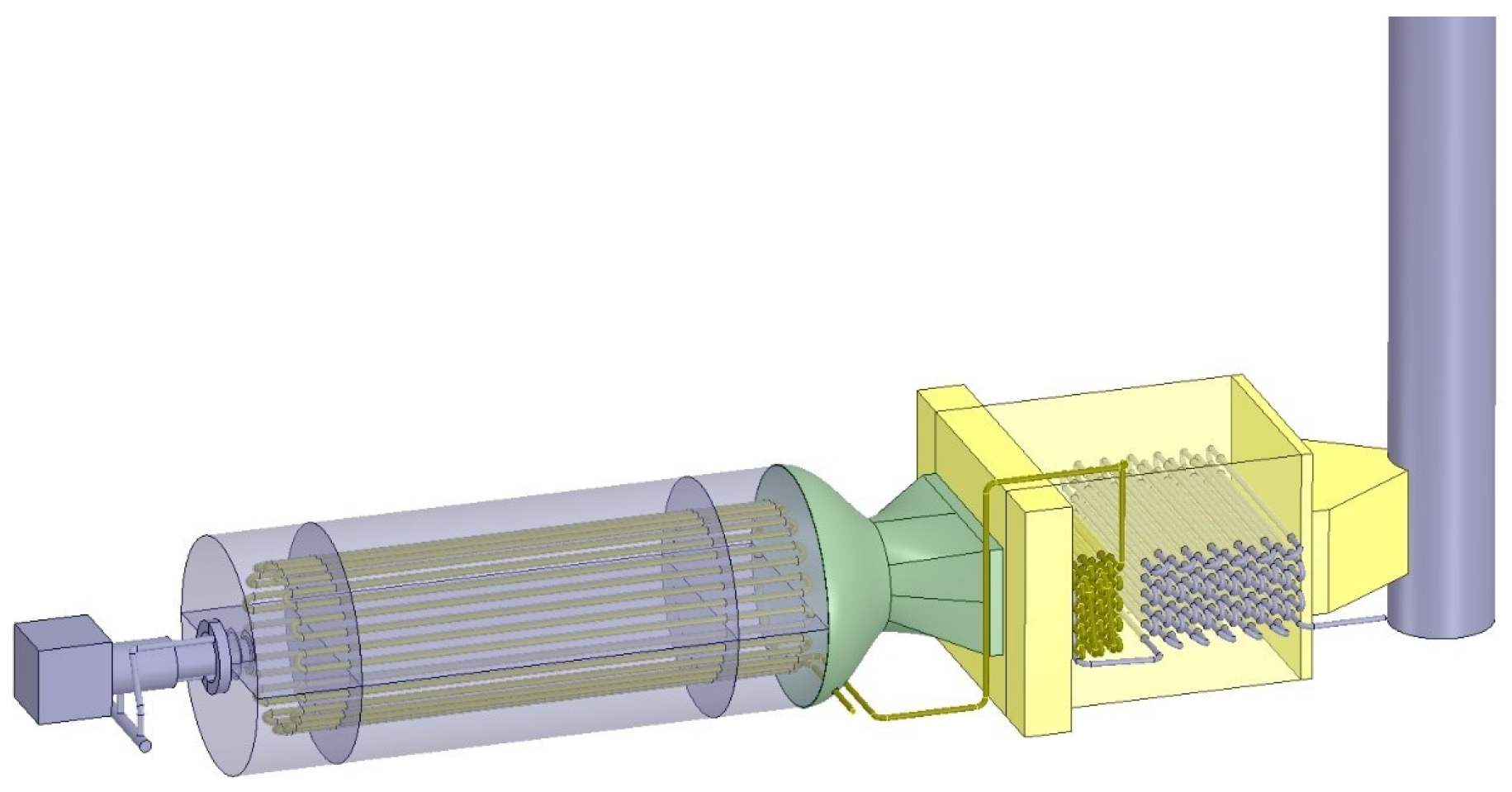
The OTSG for this research is on the pilot scale. The schematic of the OTSG is shown in Figure 1. In it, the burner is on the left, where the fuel and air are mixed, reacted, and combustion takes place. The first section of the OTSG is called the radiant section since the primary mechanism of heat transfer is radiation at this location. After the radiant section, the flue gas enters the second part of OTSG (convection section), where heat is transferred primarily through convection.

The OTSG operations specs aim to achieve the wet steam of 80–90% steam quality (by mass). For this purpose, Boiler Feed Water (BFW) enters the horizontal convection section of the OTSG, where heat is exchanged from flue gases to the water running through the tubes. As illustrated in Figure 2, the BFW travels through a series of the finned tubes (Second Tubes in Figure 2) prior to exiting the OTSG and jumping to the first row of smooth tubes (First Tubes in Figure 2) closest to the OTSG flame. The BFW then run in co-current flow with the flue gases until it reaches the last row of smooth tubes and exits the convection section. The BFW then enters the radiant tube section located closest to the burner where the radiant heat from the burner flame further heats the water until the desired outlet steam quality is achieved.

The problem is split into two, a first part focused on the combustion (Fireside) and second part focused on the steam generation inside the tubes (Waterside).

Table 1. OTSG characteristics.

Item	Description
Size	Pilot scale
Firing rate	1.7 MW
Burner type	Free-Jet
Target steam quality	80%

summarizes the key characteristic parameters in the OTSG which is modeled in the current work.

Table 2. Operating conditions of the OTSG.

Parameter	Value
Fuel inlet mass flow	0.0345 kg/s
Combustion air inlet mass flow	0.67 kg/s
Combustion air inlet temperature	75 ${}^{°}$C
Fuel inlet temperature	40 ${}^{°}$C
Stack outlet pressure	Atmospheric

shows the key process operating parameters and

Table 3. Fuel gas composition.

Component		mol. %
Hydrogen	${\mathrm{H}}_2$	0.04
Methane	${\mathrm{CH}}_4$	92.46
Ethane	${\mathrm{C}}_2{\mathrm{H}}_6$	5.85
Propane	${\mathrm{C}}_3{\mathrm{H}}_8$	1.64

points out the fuel composition feeding to the burner in Fireside of the CFD model.

3. Mathematical Model

In an OTSG, numerous transport phenomena are present. In this section we list all the governing equations that are required to characterize the system.

The mathematical details of each part of the model are not mentioned here, and more information on the constituent parts can be obtained from the respective references. A brief explanation is brought here to summarize the governing equations as follows:

3.1. Fireside (Combustion CFD Model)

The combustion CFD model was solved using commercial software ANSYS Fluent, using three-dimensional Reynolds Averaged Navier Stokes (RANS) equation with Realizable model of turbulence.

Since the flow inside the furnace would be fully turbulent, the Realizable k-$ϵ$ turbulence model (Shih et al. [14]) was employed for the present simulation. This is an empirical model based on the transport equations for turbulence kinetic energy (k) and the dissipation rate ($ϵ$), and is suitable for predicting the flows involving high shear flow spreading.

In the combustion CFD model, the energy governing equation plays an important role as it resolves the temperature distribution in the computational domain. In the Partial Differential Equation (PDE) of energy, the two source terms correspond to the radiation heat flux and the chemical reaction.

The Discrete Ordinance (DO) Model was used to model the radiation in the energy equation. The DO Model (Carvelho et al. [15]) considers the radiative transfer equation. The absorption coefficient for the gas mixture was computed using the Weighted-Sum-of-Grey-Gases (WSGGM) model (Coppalle and Vervisch [16]).

As air and fuel are multicomponent flows in the model and combustion reactions take place in the furnace where fuel and air mix, species transport equation is an essential part of any combustion CFD model. A five-step combustion mechanism (

Table 4. Five-step combustion mechanism [17].

Reaction	Arrhenius Expression
${\mathrm{CH}}_4+\frac{3}{2}{\mathrm{O}}_2\to \mathrm{CO}+2{\mathrm{H}}_2\mathrm{O}$	$R_{i,1}=1.0\times {10}^{10}\exp \left(\frac{-125,604}{RT}\right){\left[C{H}_4\right]}^{-0.3}{\left[O_2\right]}^{1.3}$
${\mathrm{C}}_2{\mathrm{H}}_6+\frac{5}{2}{\mathrm{O}}_2\to 2\mathrm{CO}+3{\mathrm{H}}_2\mathrm{O}$	$R_{i,2}=1.0\times {10}^{12}\exp \left(\frac{-125,604}{RT}\right){\left[C_2{H}_6\right]}^{0.1}{\left[O_2\right]}^{1.65}$
${\mathrm{C}}_3{\mathrm{H}}_8+\frac{7}{2}{\mathrm{O}}_2\to 3\mathrm{CO}+4{\mathrm{H}}_2\mathrm{O}$	$R_{i,3}=1.0\times {10}^{12}\exp \left(\frac{-125,604}{RT}\right){\left[C_3{H}_8\right]}^{0.1}{\left[O_2\right]}^{1.65}$
$\mathrm{CO}+\frac{1}{2}{\mathrm{O}}_2\to {\mathrm{CO}}_2$	$R_{i,4}=1.0\times {10}^{14}\exp \left(\frac{-167,472}{RT}\right)\left[CO\right]{\left[H_{2}O\right]}^{0.5}{\left[O_2\right]}^{0.25}$
${\mathrm{H}}_2+\frac{1}{2}{\mathrm{O}}_2\to {\mathrm{H}}_2\mathrm{O}$	$R_{i,5}=1.0\times {10}^{15}\exp \left(\frac{-100}{RT}\right)\left[H_2\right]\left[O_2\right]$

), combined with the Eddy-Dissipation Model (EDM) and finite rate models was chosen to simulate the combustion, based on the kinetics of Westbrook and Dryer [17]:

It is worthwhile to mention that the the heat transfer resistances associated to conduction for the wall of tubes were assumed to be zero and, thus, no conduction model was considered for the tube walls. Additionally, no boundary layers cell was taken into account in the mesh grid. These simplification assumptions were performed in the model to reduce the mesh complexity and optimize the computational time. In addition, the effect of buoyancy force was neglected since this particular OTSG is horizontal.

The PDEs of combustion CFD model in Fireside along with the corresponding submodels are shown in

Table 5. Governing equations of Fireside [18].

Equation	Formulation
Continuity (single-phase)	$\frac{\partial \rho }{\partial t}+\nabla · \left(\rho \mathbf{U}\right)=0$
Momentum (single-phase)	$\frac{\partial }{\partial t}\left(\rho \mathbf{U}\right)+\nabla ·\left(\rho \mathbf{U}\mathbf{U}\right)=-\nabla p+\nabla ·{\overline{\overline{\tau }}}_{\mathrm{effi}}$
Reynolds stress tensor	${\overline{\overline{\tau }}}_{\mathrm{effi}}=\left({\mu }_{\mathrm{lam}}+{\mu }_{\mathrm{t}}\right)\left(\nabla \mathbf{U}+\nabla {\mathbf{U}}^T\right)-\frac{2}{3}\left(\rho k+\left({\mu }_{\mathrm{lam}}+{\mu }_{\mathrm{t}}\right)\nabla ·\mathbf{U}\right)\overline{\overline{I}}$
Realizable k-$ϵ$ model	$\frac{\partial }{\partial t}\left(\rho k\right)+\nabla ·\left(\rho \mathbf{U}k\right)=\nabla ·\left(\frac{\mu }{{\sigma }_{\mathrm{k}}}\nabla k\right)+G_k+G_b-\rho ϵ-Y_M+S_k$
	$\frac{\partial }{\partial t}\left(\rho ϵ\right)+\nabla ·\left(\rho \mathbf{U}ϵ\right)=\nabla ·\left(\frac{{\mu }_{\mathrm{t}}}{{\sigma }_{\mathrm{ffl}}}\nabla ϵ\right)+\rho C_{1}Sϵ-\rho C_2\frac{{ϵ}^2}{k+\sqrt{\nu ϵ}}+G_{ϵ}\frac{ϵ}{k}{C}_{3ϵ}{G}_b+S_{ϵ}$
	$C_1=max\left[0.43,\frac{\eta }{\eta +5}\right]$, $\eta =S\frac{k}{ϵ}$, $S=\sqrt{2S_{ij}{S}_{ij}}$
Energy equation	$\frac{\partial }{\partial t}\left(\rho E\right)+\nabla ·\left(\rho \mathbf{U}E\right)=\nabla ·(k+k_t·\nabla T)+\nabla ·(\tau ·\mathbf{U})+\nabla ·\left(p\mathbf{U}\right)+S_r+S_k$
DO model	$\nabla ·\left(I(\overrightarrow{r},\overrightarrow{s})\right)\overrightarrow{s}+(a+{\sigma }_s)I(\overrightarrow{r},\overrightarrow{s})=a{n}^2\frac{\sigma T^4}{\pi }+\frac{{\sigma }_s}{4\pi }{\int }_0^{4\pi }I(\overrightarrow{s},\overrightarrow{s^{\prime }})d{\mathrm{\Omega }}^{\prime }$
Species transport equation	$\frac{\partial }{\partial t}\left(\rho m_l\right)+\nabla ·\left(\rho \mathbf{U}{m}_l\right)=\nabla ·\left((\rho D+\frac{{\mu }_t}{{\sigma }_m})\nabla m\right)+R_l$
EDM model	$R_{i,r}={\nu }_{i,r}^{\prime }{M}_{w,i}A\rho \frac{ϵ}{k}{\min }_{\Re }\left(\frac{Y_R}{{\nu }_{\Re ,r}^{\prime }{M}_{w,\Re }}\right)$
	$R_{i,r}={\nu }_{i,r}^{\prime }{M}_{w,i}AB\rho \frac{ϵ}{k}\left[\frac{{\mathrm{\Sigma }}_p{Y}_p}{{\mathrm{\sum }}_j^N\nu {″}_{j,r}{M}_{w,j}}\right]$

. Additionally,

Table 6. Basic setup of CFD model in ANSYS Fluent (Fireside).

Model	Type or/and Value
Turbulence	realizable k-$ϵ$ model
Wall function	non-equilibrium
Radiation	DOM
Gas absorption properties	grey-gas model
Combustion	5-step mechanism EDM/Finite rate model
Heat Transfer towards Tubes	steam/water temperature and inside heat transfer coeff.
Tube metal	emissivity = 0.85
Burner tile	adiabatic; emissivity = 0.65
Transition from the convection section to stack	adiabatic; emissivity = 0.65
Refractory walls of the radiant section and the convection section	adiabatic; emissivity = 0.65
Stack walls	adiabatic; emissivity = 0.65

indicates more details regarding the basic combustion CFD submodels and their configuration.

3.2. Waterside (Multiphase CFD Model)

Inside the steam tubes placed in the convection and the radiant sections of the OTSG, a multiphase CFD approach should be adopted as BFW is converted to steam due to the exerted heat fluxes on the tubes originating from Fireside.

Here, the goal is to apply a multiphase CFD model which is applicable at an industrial scale. For this model to be computationally and industrially usable, the micro scale models are not efficient and a macro scale model is required.

In the current study, a Eulerian–Eulerian approach (E-E) is selected as it falls under the category of macro scale models. The E-E model is applied when a relatively large number of particles (bubbles/droplets) with a continuous phase exists in the system. Although the E-E model consumes less computational power, it requires an adequate closure relation for the interfacial coupling terms (i.e., drag and lift forces) and phase change with the presence of boiling in the system.

The boiling physics involved in the present system is complex. Due to the complexity and the lack of validated theoretical models, most boiling models are based on sets of hard to obtain experimental correlations, and their closure parameters are often extremely sensitive to the geometry and type of problems. There is only one reliable model for boiling available, the outcome of continued research and development efforts at the Rensselaer Polytechnic Institute (RPI) called the RPI boiling model (Kurul and Podowski [19]).

The multiphase CFD model was built using commercial software ANSYS CFX, using three-dimensional Eulerian–Eulerian equations with mixture k-$ϵ$ model of turbulence.

The PDEs of the multiphase CFD model in Waterside along with the corresponding submodels are shown in

Table 7. Governing equations of Waterside [22].

Equation	Formulation
Continuity	$\frac{\partial }{\partial t}\left({\rho }_{\mathrm{i}}{\alpha }_{\mathrm{i}}\right)+\nabla ·\left({\alpha }_{\mathrm{i}}{\rho }_{\mathrm{i}}{\mathbf{U}}_{\mathrm{i}}\right)={\mathsf{\Gamma }}_{ij}^{+}-{\mathsf{\Gamma }}_{ji}^{+}$
Momentum	$\frac{\partial }{\partial t}\left({\rho }_{\mathrm{i}}{\alpha }_{\mathrm{i}}{\mathbf{U}}_{\mathrm{i}}\right)+\nabla ·\left({\alpha }_{\mathrm{i}}{\rho }_{\mathrm{i}}{\mathbf{U}}_{\mathrm{i}}{\mathbf{U}}_{\mathrm{i}}\right)=-{\alpha }_{\mathrm{i}}\nabla p+\nabla ·\left({\alpha }_i{\overline{\overline{\tau }}}_{\mathrm{effi},i}\right)+{\mathbf{R}}_{\mathrm{i}}+{\mathbf{F}}_{\mathrm{i}}+{\alpha }_{\mathrm{i}}{\rho }_{\mathrm{i}}\mathbf{g}++({\mathsf{\Gamma }}_{ij}^{+}{\mathbf{U}}_{\mathrm{j}}-{\mathsf{\Gamma }}_{ij}^{+}{\mathbf{U}}_{\mathrm{i}})$
Reynolds stress tensor	${\overline{\overline{\tau }}}_{\mathrm{effi},\mathrm{i}}=\left({\mu }_{\mathrm{lam},\mathrm{i}}+{\mu }_{\mathrm{t},\mathrm{i}}\right)\left(\nabla {\mathbf{U}}_{\mathrm{i}}+\nabla {\mathbf{U}}_{\mathrm{i}}^T\right)-\frac{2}{3}\left({\rho }_i{k}_i+\left({\mu }_{\mathrm{lam},\mathrm{i}}+{\mu }_{\mathrm{t},\mathrm{i}}\right)\nabla ·{\mathbf{U}}_{\mathrm{i}}\right)\overline{\overline{I}}$
Interfacial momentum exchange	${\mathbf{R}}_{\mathrm{G}}=-{\mathbf{R}}_{\mathrm{L}}={\mathbf{R}}_{\mathrm{G},\mathrm{drag}}+{\mathbf{R}}_{\mathrm{G},\mathrm{lift}}+{\mathbf{R}}_{\mathrm{G},\mathrm{vm}}$
Liquid–gas exchange coefficient	$K=\frac{3}{4}{\rho }_{\mathrm{L}}{\alpha }_{\mathrm{G}}\frac{C_{\mathrm{D}}}{d_{32}}\mid {\mathbf{U}}_{\mathrm{G}}-{\mathbf{U}}_{\mathrm{L}}\mid ({\mathbf{U}}_{\mathrm{G}}-{\mathbf{U}}_{\mathrm{L}})+{\alpha }_{\mathrm{G}}{C}_{\mathrm{l}}{\rho }_{\mathrm{L}}{\mathbf{U}}_{\mathbf{r}}\times (\nabla \times {\mathbf{U}}_{\mathbf{L}})+{\alpha }_{\mathrm{L}}{C}_{\mathrm{vm}}{\rho }_{\mathrm{L}}\left(\frac{D_L{\mathbf{U}}_{\mathbf{L}}}{Dt}-\frac{D_G{\mathbf{U}}_{\mathbf{G}}}{Dt}\right)$
Ishii–Zuber drag coefficient [23]	$C_D=max\{min[\frac{2}{3}\sqrt{\mathrm{Eo}},\frac{8}{3}],\frac{24}{\mathrm{Re}}(1+0.1{\mathrm{Re}}^{0.75})\}$
Energy	$\frac{\partial }{\partial t}\left({\rho }_{\mathrm{i}}{\alpha }_{\mathrm{i}}{h}_{\mathrm{i}}\right)+\nabla ·\left({\alpha }_{\mathrm{i}}{\rho }_{\mathrm{i}}{h}_{\mathrm{i}}{\mathbf{U}}_{\mathrm{i}}\right)=\nabla ·\left[\alpha \mathrm{i}\left({\mathbf{q}}_{\mathrm{i}}+{\mathbf{q}}_{\mathrm{i}}^t\right)\right]+{\alpha }_{\mathrm{i}}\frac{DP}{Dt}+({\mathsf{\Gamma }}_{ij}^{+}{h}_{\mathrm{j}}-{\mathsf{\Gamma }}_{ij}^{+}{h}_{\mathrm{i}})+Q_i+q_{\mathrm{wall}}^{″}{A}_{\mathrm{wall}}^{″}$
	${\mathbf{q}}_{\mathrm{i}}=-\frac{{\lambda }_i}{C_{p,i}}\overrightarrow{\nabla }{h}_{\mathrm{i}}{\mathbf{q}}_{\mathrm{i}}^t=-\frac{{\lambda }_i^t}{C_{p,i}}\overrightarrow{\nabla }{h}_{\mathrm{i}}$
	${\mathsf{\Gamma }}_{\mathrm{ij}}^{+}=\frac{q_{\mathrm{wall}}^{e″}}{h_{tv}}A{″}_{\mathrm{wall}}$
	${\mathsf{\Gamma }}_{\mathrm{ji}}^{+}=\frac{h_{\mathrm{int}}\left(T_{\mathrm{sat}}-T_b\right)a_{\mathrm{int}}}{h_{\mathrm{tv}}}$
RPI boiling model	$q{″}_{\mathrm{wall}}=q_{\mathrm{wall}}^{c″}+q_{\mathrm{wall}}^{e″}+q_{\mathrm{wall}}^{q″}$
	$q_{\mathrm{wall}}^{c″}=h_c(T_w-T_l)(1-A_b)$
	$q_{\mathrm{wall}}^{q″}=\frac{2K}{\sqrt{\pi {\lambda }_{l}T}}(T_w-T_l)$
	$q_{\mathrm{wall}}^{e″}=V_d{N}_w{\rho }_{\nu }{h}_{\mathrm{fv}}$
Tomiyama lift coefficient [24]	$C_l=\left\{\begin{array}{c}min(0.288tanh\left(0.121\mathrm{Re}\right),f\left({\mathrm{Eo}}_G\right)){\mathrm{Eo}}_G<4\hfill \\ f\left({\mathrm{Eo}}_G\right)4\le {\mathrm{Eo}}_G\le 10.7\hfill \end{array}\right.$
Mixture k-$ϵ$ model [25]	$\frac{\partial }{\partial t}\left({\rho }_{\mathrm{m}}{k}_{\mathrm{m}}\right)+\nabla ·\left({\rho }_{\mathrm{m}}{\mathbf{U}}_{\mathrm{m}}{k}_{\mathrm{m}}\right)=\nabla ·\left(\frac{{\mu }_{\mathrm{t},\mathrm{m}}}{{\sigma }_{\mathrm{k}}}\nabla k_{\mathrm{m}}\right)+P_k^{\mathrm{m}}-{\rho }_{\mathrm{m}}{ϵ}_{\mathrm{m}}+S_k^{\mathrm{m}}$
	$\frac{\partial }{\partial t}\left({\rho }_{\mathrm{m}}{ϵ}_{\mathrm{m}}\right)+\nabla ·\left({\rho }_{\mathrm{m}}{\mathbf{U}}_{\mathrm{m}}{ϵ}_{\mathrm{m}}\right)=\nabla ·\left(\frac{{\mu }_{\mathrm{t},\mathrm{m}}}{{\sigma }_{ϵ}}\nabla k_{\mathrm{m}}\right)+\frac{{ϵ}_m}{k_m}\left(C_{1ϵ}{G}_{\mathrm{k},\mathrm{m}}-C_{2ϵ}{\rho }_{\mathrm{m}}{ϵ}_{\mathrm{m}}\right)+C_{ϵ3}\frac{{ϵ}_m}{{ϵ}_k}{S}_k^{\mathrm{m}}$

. For further details about boiling and two-phase flow, readers are referred to Askari [20] and Rabiee [21].

Table 8. Basic setup of CFD Model in ANSYS CFX (Waterside).

Model	Type or/and Value
Turbulence	Mixture k-$ϵ$ model
Drag coefficient	Ishii-Zuber
Lift coefficient	Tomiyama lift coefficient
Boiling	RPI model
Bubble size model	constant (${\mathrm{d}}_{\mathrm{o}}=5\mathrm{mm}$)

summarizes the basic submodels and configuration of the developed two-phase CFD model.

3.3. Coupling between Waterside (Multiphase CFD) and Fireside (Combustion CFD)

A strong coupling between the CFD modeling of both Fireside and Waterside of the OTSG is desired in this work. Each model is connected to form a full system model of OTSG where the inputs and results from each can be automatically used interchangeably between them.

As combustion CFD in the furnace calculates the heat fluxes on the tubes, the multiphase CFD captures the heat transfer coefficient and temperature of the steam inside the tube. Hence, the parameters which have a duty to establish the coupling between Fireside and Waterside are as follows:

• Heat fluxes (from Fireside);
• Heat transfer coefficient and Temperature (from Waterside).

The coupling is provided by equation below:

$$q″=h(T-T_{\infty })$$

(1)

where $q″$ is heat flux calculated by combustion CFD, $T_{\infty }$ is process fluid (BFW) temperature and h is the heat transfer coefficient of the flow inside the tubes. The $q″$ stands for the boundary condition in multiphase CFD model, while h and $T_{\infty }$ are used to form the boundary condition for combustion CFD part. Figure 3 and Figure 4 display the coupling algorithm and the schematic of the degree of coupling, respectively.

4. CFD Model Setup

4.1. Geometrical Model

The following simplification features were adopted to create the geometry for the CFD model:

1.

The structural members (beams, etc.) inside the furnace were not modeled. They do not take part into the fluid flow simulation, and the effect of their presence is assumed to be negligible;

2.

The inlet boundaries of the simulation are the air inlet duct to the windbox and the fuel pipe inlet. It is assumed that the flow is steady and homogeneous;

3.

For this particular case, the burner model consists of the two burner tips. One half circle is type 1 burner tips and another half circle is the type 2 burner tips according to the burner manufacture drawings. Type 1 burner tips direct the fuel jet inward (Figure 5) while Type 2 burner tips jet the gas parallel to the centerline or slightly outward (Figure 6).

4.

The outlet of the simulation was cut off after the end point of stack where the flue gas exit joins with the stack. Atmospheric pressure was applied at the stack outlet;

5.

All furnace surfaces were assumed to be adiabatic with a specific radiant emissivity;

6.

For the sake of simplicity, the geometry of finned tubes was not considered in the geometry model. The computational time would be substantially increased without this simplification. Instead, the equivalence diameter approach for finned tubes was adopted, thus the physical shape of individual fins is not included in the solid model.

Figure 5. Burner type 1 schematic.

Figure 5. Burner type 1 schematic.

Figure 6. Burner type 2 schematic.

Figure 6. Burner type 2 schematic.

Figure 7 demonstrates the geometry used in the OTSG CFD model development.

4.2. Mesh Generation

The discretization of the geometry utilized high order elements. The resulting mesh cell count is shown in

Table 9. Mesh statistics.

Assembly	No. Cells
Burner-Radiant section (Fireside)	33 M
Convective-Stack section (Fireside)	6 M
First Tubes (Waterside)	12 M
Second Tubes (Waterside)	13 M
Radiant Tubes (Waterside)	14 M

.

The meshed geometry is shown in Figure 8, Figure 9 and Figure 10. The whole geometry was broken into two general assemblies for Fireside and three assemblies for Waterside and mesh was generated separately for each part. After completion of mesh generation, the merging tool in ANSYS Fluent was used to connect the two meshes in Fireside section. This approach optimized the mesh processing time and provided one single mesh grid for Fireside computational domain.

4.3. Solution Strategy

A single-node cluster containing four Intel Xenon CPUs with four cores running at 3.2 GHz was used to run the simulations. This cluster was equipped with a memory of 64 Gb per CPU meaning 256 Gb in total.

The simulation on Fireside was initialized using the Hybrid-Initialization of ANSYS Fluent and started without combustion reactions no the radiation model. The simulation was run to capture a stable behavior in terms of velocity and energy residuals. In the second step, the ignition process was performed to include the combustion reactions in the domain. To ignite, a spherical volume was defined next to burner tiles and given small values of combustion products with a high temperature (3000 ${}^{°}$C).

The simulation was restarted with a very low under-relaxation density factor, and as the solution progresses, the under-relaxation factors were slowly increased to ensure that the solution achieved a stable state. In the last step, the radiation model was activated and the simulation process was launched to reach the end point. The complete Fireside simulation required 500 h of wall-clock time to run. In addition to monitoring the velocity, energy, and species residuals, the net mass and energy imbalance of the simulation were also monitored.

Once the combustion CFD model was converged, the heat fluxes on the tube surfaces were computed and passed to Waterside two-phase simulation as boundary conditions. In two-phase flow CFD simulation, the value of the vapor phase fraction at the tube outlet was being monitored to confirm the simulation convergence. A breakdown of wall-clock time for Waterside is shown in

Table 10. Breakdown of wall-clock time for Waterside simulation.

Assembly	Approximate Wall-Clock Time [h]
First Tubes (convection section)	120
Second Tubes (convection section)	300
Radiant Tubes	320

.

5. Results and Discussion

5.1. Validation

In the first validation step, the composition of combustion products was compared to field data. It was found that the CFD results are in good agreement with field values as the pie charts in Figure 11 show:

As

Table 11. Comparison between field datasheet and CFD results in the radiant section.

Parameter	Field Data	CFD
Average radiant section flux [kW/m${}^2$]	52.77	47.576
Flue gas temperature leaving the radiant section [${}^{°}$C]	1144	1152.18

and

Table 12. Comparison between heat fluxes for field datasheet and CFD model in First Tubes.

Tube ID	Field Data [kW/m${}^2$]	CFD [kW/m${}^2$]
$\#1$	52.96	51.85
$\#2$	30.57	24.5

indicate, there is a fair agreement in terms of heat flux between the field datasheet and CFD model in the radiant section and the first group of convection tubes (First Tubes). However, the third column of

Table 13. Comparison between heat fluxes for field datasheet and CFD model in Second Tubes.

Tube ID	Field Data [kW/m${}^2$]	CFD (w/o Fins) [kW/m${}^2$]	CFD (with Fins) [kW/m${}^2$]
$\#3$	54.06	20.85	50.6
$\#4$	29.87	17.78	28.61
$\#5$	13.30	16.18	17.17

demonstrates a discrepancy for heat fluxes on the second group of tubes (Second Tubes). This difference corresponds to the fins geometry simplification as explained in Section 4.1. The fourth column of Table 13 shows a comparison of heat fluxes when a detailed model of the fins is considered in the CFD model. Although the addition of fins geometry substantially complicates the mesh network and consequently increases the computational time, it leads to improvement in heat fluxes of fined tubes in the simulation. The details of this additional CFD analysis will be discussed further in Section 5.

5.2. Coupling

A strong coupling between Waterside and Fireside was established using the algorithm shown in Figure 3.

Table 14. Comparison among three iterations in coupling section.

Tube Number	${\mathbf{q}″}_{\mathbf{intial}\mathbf{point},\mathbf{furnace}-5}[\mathbf{kW}/{\mathbf{m}}^2]$	${\mathbf{q}″}_{\mathbf{first}\mathbf{iteration}}[\mathbf{kW}/{\mathbf{m}}^2]$	${\mathbf{q}″}_{\mathbf{second}\mathbf{iteration}}[\mathbf{kW}/{\mathbf{m}}^2]$
#1	9612	16,932	16,839
#2	9509	16,772	16,683
#3	9408	16,552	16,454
#4	9310	16,748	16,635
#5	9212	16,962	16,855
#6	9112	17,003	16,886
#7	12,073	16,689	16,581
#8	11,971	16,847	16,746
#9	11,871	16,821	16,709
#10	11,774	16,339	16,223
#11	11,676	16,629	16,518
#12	11,574	16,807	16,682
#13	15,361	17,739	17,629
#14	15,193	17,842	17,716
#15	15,029	17,969	17,850
#16	14,864	17,985	17,855
#17	14,701	18,022	17,897
#18	14,540	18,080	17,943
#19	19,421	17,351	17,249
#20	19,260	17,341	17,246
#21	19,094	17,395	17,291
#22	18,936	17,501	17,402
#23	18,783	17,516	17,425
#24	18,626	17,574	17,469

indicates the model coupling with respect to the calculated heat fluxes over three loops/cycles. It is worthwhile to mention that, to speed up the convergency, a 1-D software (Furnace-5) was employed to provide the initial heat fluxes in the model. Table 14 confirms that the coupling is achieved within an acceptable accuracy in the first loop (the second column). The reason is the accurate initialization values that were obtained from 1-D software.

5.3. Results

Figure 12, Figure 13 and Figure 14 display the temperature and velocity profile through a vertical cuts inside the OTSG domain. These figures represent the shape of the jet in the radiant section. The flue gas passing the transition zone entering the convective section has a considerably high temperature, which is the consequence of combustion and the heat production in the radiant section. The prediction of the blue zone in the middle of the convective section confirms the cooling effect imposed by BFW entering the tubes of the convective part. Then, the flue gas coming from the convective section enters the stack and moves upwards with a fixed temperature due to exposure to the adiabatic stack surface.

An analysis on the convection box with a more detailed model of the fins was performed and it concludes that fins addition drops the stack temperature (Figure 15). The fins in this analysis modeled as baffles. A baffle is recognized as a zero-thickness wall. The conduction resistance of the wall fins was neglected to simplify the model and no conduction term was taken into account in the wall boundary condition in the fin/tube. The lack of heat absorption is not entirely captured on the tubes without consideration of fins geometry. It is plausible to attribute this issue to the absence of detailed fin geometry on the tubes in the model. The presence of fins leads to additional disruption of the gas-side flow (Figure 16), and enhances the heat transfer characteristics of the fin. The trade-off for this enhanced performance is increased pressure loss.

Figure 17 illustrates the duty distributions within OTSG volume. If the effect of fins is not present in the CFD model, the radiant section and the convection section absorb 43% and 36% of the input duty, respectively. The addition of fins geometry to the CFD model increases the absorbed heat in the radiant section by 10%.

Table 15. Duty distribution and overall OTSG comparison between field datasheet and CFD model.

	Absorbed Heat Rate at Radiant Section [MW]	Absorbed Heat Rate at Convection Section [MW]	Overall OTSG Efficiency %
Field data	0.71	0.834	90.8
CFD (w/o fins)	0.735	0.617	79
CFD (with fins)	0.735	0.806	90.6

summarizes an overall comparison between field data and CFD simulation results with respect to absorbed heat transfer in the radiant section, the convection section, and overall OTSG efficiency. Table 15 confirms that the overall OTSG efficiency that the CFD model obtains matches the reported OTSG efficiency in the field datasheet.

The tile temperature should be above the autoignition temperature of the fuel otherwise it may lead to flame instability. Autoignition Temperature (AIT) is defined as the temperature at which vapors ignite spontaneously from the heat of the environment. Figure 18 depicts that the tile temperature is higher than AIT of the fuel (i.e., 810.15 ${}^{°}$K). This finding concludes that flame instability is not present in this particular burner under the stated operating conditions.

As mentioned earlier, the mass flow inlet was defined as the boundary condition. Consequently, the CFD model calculated the pressure at fuel inlet. CFD results show that the fuel inlet pressure is 24.37 psi which is in the available pressure range for the fuel line in the refineries. The pressure of fuel line can assist burner designers for fuel port sizing if the fuel composition is known (API-560 [26]).

According to industry accepted definition, the flame is visualized based on the iso contour of 2000 ppm CO. That means 99.8% combustion is completed within the flame. Figure 19 visualizes the flame based on the iso-surface of 2000 ppm CO concentration. The volume average of CO concentration at the convection section (6.84 ppm) is smaller than 10 ppm (Figure 20). This shows that the spontaneous combustion is not possible in the convection section. However, the flame shape shown in Figure 19 is an indication of flame impingement in the furnace. The presence of oxygen confirms the presence of flame within the long distance from the burner tips and the end of the radiant section.

CFD results are post-processed to determine the Tube Metal Temperature (TMT).

Table 16. Comparison between maximum TMTs per design and TMTs per CFD results.

Tube ID	Max. TMTs [${}^{°}$C] Coil Design Datasheet	Max. TMTs [${}^{°}$C] CFD
$\#1$	395.3	338.3
$\#2$	347.5	324.4
$\#3$	347.5	328.2
$\#4$	377.4	265.1
$\#5$	377.4	222
$\#6$	377.4	200

illustrates that TMTs from CFD is lower than Maximum TMTs which satisfies tube/coil design condition. The maximum TMTs that are found in the coil design datasheet cannot be exceeded. The tube temperature should be below the maximum TMT to avoid metallurgical issues.

Figure 21 provides the radiative heat flux over the radiant tubes. This contour profile shows that the heat absorbent in the tube backside is lower than their frontside surfaces (blue as the dominant color in the backside surfaces).

Here, the circumferential flux factor (CFF) needs to be calculated. The CFF is defined as the maximum to average radiation flux ratio in the radiant section. The CFF should be around 1.2–1.3 since the backside of the tube absorbs heat by indirect radiation from the refractory and the frontside experiences the direct radiation. Additionally, the tube metal emissivity is 0.85 while the refractory walls of the radiant section have the emissivity of 0.65 (Table 6). This means that the refractory walls of radiant section absorb a lower amount of radiative heat compared to the tube metal surface. Since the tube backside only sees the refractory walls of the radiant section, it cannot receive the same amount of radiative energy as the tube frontside. Thus, by the radiant tube backside is cooler than the radiant tube frontside.

As CFF value approaches unity, the improvement in the radiant efficiency is increased.

Table 17. CFF values at the three locations of the radiant section.

Zone #	Maximum [kw/m${}^2$]	Average [kw/m${}^2$]	CFF
$\#1$	30.56	19.7	1.5
$\#2$	68.5	28.15	2.43
$\#3$	129.4	59.07	2.91

exhibits the CFF values at the three locations which are identified in Figure 22. As the calculated CFF values are considerably higher than unity, it can be concluded that the radiant section is not optimized. This can lead to a decrease in the OTSG efficiency.

The steam generation through the pipes was modeled and then coupled with the flue gas side using those heat fluxes predicted by the combustion CFD model on the tube surfaces. The results are shown in Figure 23, Figure 24, Figure 25, Figure 26, Figure 27, Figure 28 and Figure 29.

For the convective part as shown in Figure 23, Figure 24 and Figure 25, at the elbows most of the vapor remains towards the intrados of the elbow, whereas the remaining liquid resides at the extrados of the elbow. The distribution is more drastic for Second Tubes due to the presence of more liquid compared to the radiant section (Figure 26 and Figure 27).

When approaching the elbow, most of the vapor occupies the upper portion of the pipe due to the buoyancy effect. Similarly, at the elbow, most of the vapor resides at the intrados of the elbow due to the centrifugal force acting on the vapor particles. To understand this flow behavior holistically,

Table 18. Bulk velocity values at the BFW inlet and the radiant section outlet.

	Steam Quality	Bulk Velocity [m/s]
BFW inlet (OTSG inlet)	0%	1.6
Radiant section outlet (OTSG exit)	80%	18

provides the representative bulk velocities at the BFW inlet (OTSG inlet) and the radiant section outlet (OTSG exit). The increase in the bulk velocity along the axial direction of the tubes leads to the tendency of the vapor phase towards the intrados.

Liquid Droplet Impingement (LDI) erosion could be regarded to be one of the major causes of unexpected troubles occasionally occurring in the inner bent pipe surface. The bent pipe wall thinning phenomena might be an issue at the elbow of the pipes as Li et al. [27] showed in their study.

The model results predict the location where evaporation starts in First Tubes in the convection section. The vapor volume fraction contour from row 15 in First Tubes shows the bubbly flow and the transition from single phase to two-phase flow (Figure 28). Figure 29 illustrates the temperature contour from row 14 in the convective section where the water temperature approaches the saturation value.

6. Cost and Benefit of CFD Approach

The main benefit derived from performing CFD in relation to OTSGs is the reduction in cost achieved when developing new designs or in the design of modifications aimed at increasing throughput or efficiency. In the traditional design approach, extensive testing is required to confirm the design meet certain performance standards, including heat transfer, minimum emissions, flame orientation, and flame stability. Testing informs the iterative design process and in most practical cases full-scale testing is not feasible, leaving room for uncertainties.

Table 19. Comparison of cost/benefit between CFD approach and OTSG traditional design approach.

Project Type	Timeframe	Cost
Traditional design approach [28]	2 years	$2 M
CFD approach	up to 12 months	$500 K–$750 K (based on industrial experience)

shows a cost comparison between a CFD approach which was studied as an example. Based in our experience the estimated shortening of the design cycle and the shortening of the timeline are in line with those put forward by Charles and Baukal [28]. The CFD simulation decreases the traditional OTSG design cost by a minimum 75% and shortens the development cycle by an estimated 20% (Charles and Baukal [28].

7. Conclusions

A complete CFD model of the combustion in an OTSG was performed. The results represented the shape of the jet and showed that the flue gas goes through the transition part and passes over the convective tubes and then reaches the entrance of the stack. Then, the gas moves upwards to exit at the stack outlet. The temperature profiles indicated that the flue gas passing the transition zone and entering the convective section have a considerable high temperature (1152.8 ${}^{°}$C), which is the consequence of combustion and the heat production in the radiant section.

The prediction of a low temperature zone in the middle of the convective section confirms the cooling effect imposed by BFW entering the tubes of the convective part. Then, the flue gas coming from the convective section enters the stack and moves upwards with a fixed temperature due to the exposure of the adiabatic surface of the stack.

First, the CFD results were compared to available field data for which a good agreement of our model results was found. In the next step, it was shown that CFD simulation is able to predict the flame shape and orientation. The CFD results were post-processed to study the possibility of flame instability. Additionally, the split between radiative duty and convective duty was assessed to inspect the radiation and the convection efficiency inside the OTSG. The fuel flow rate at the fuel inlet was determined from the model outputs and it was found that the fuel flow rate value lies on an acceptable refinery range. The temperature distribution on the radiation/convection tube walls showed that the maximum tube temperature does not exceed the design temperature.

An analysis with the inclusion of fins geometry on the second bank of tubes of the convection box was performed. This analysis indicated that the addition of fins to our model improves the results as it drops the flue gas temperature at the stack outlet. The increased pressure loss caused by the fins in flue gas flow is the main reason for the temperature drop in the stack.

Results of the steam generation model showed the majority of the vapor remains towards the intrados of the elbow, whereas the remaining liquid resides at the extrados of the elbow. On the other side, while approaching the elbow most of the vapor occupies the upper portion of the pipe due to the buoyancy effect. Similarly, at the elbow, most of the vapor resides at the intrados of the elbow due to the centrifugal force acting on the vapor particles.

This work confirmed a CFD approach can shorten the traditional process timeline for an industrial OTSG design and reduce its associated design cost.

References

1. Charles, E.; Baukal, J. The John Zink Hamworthy Combustion Handbook; CRC Press: Boca Raton, FL, USA, 2013. [Google Scholar]
2. Khoshhal, A.; Rahimi, M.; Alsairafi, A.A. The CFD Modeling of NOx Emission, HiTAC and Heat Transfer in an Industrial Boiler. Numer. Heat Transf. Part A Appl. 2010, 58, 295–312. [Google Scholar] [CrossRef]
3. Thornock, J.N.; Spinti, J.P.; Hradisky, M. Evaluating the NOx Performance of a Steam Generator for Heavy Oil Production; American Flame Research Committee: Houston, TX, USA, 2014. [Google Scholar]
4. Liu, B.; Wang, Y.-H.; Xu, H. Numerical Study of the Effect of Staged Gun and Quarl on the Performance of Low-NOx Burners. J. Energy Eng. 2016, 142, 04015040. [Google Scholar] [CrossRef]
5. Ye, K.; Zhang, Y.; Lin, J.; Li, N.; Yang, Y.; Li, Z.; Hao, J.; Chen, Y. CFD Analysis of the Primary Side in a Helical-Coil Once-Through Steam Generator. In Proceedings of the 2017 25th International Conference on Nuclear Engineering, Shanghai, China, 2–6 July 2017. [Google Scholar] [CrossRef]
6. Liu, B.; Bao, B.; Wang, Y.; Xu, H. Numerical simulation of flow, combustion and NO emission of a fuel-staged industrial gas burner. J. Energy Inst. 2017, 90, 441–451. [Google Scholar] [CrossRef]
7. Singha, A.; Forcinito, M. Emission Characteristic Map and Optimization of NOx in 100 MW Staged Combustion Once-Through-Steam-Generator (OTSG). In Proceedings of the AFRC Indsutrial Combustion Symposium, Salt Lake City, UT, USA, 17–19 September 2018. [Google Scholar]
8. Singha, A.; Forcinito, M. Modelling Different Aspects of Once though Steam Generators. In Proceedings of the NAFEMS World Congress (NWC), Quebec City, QC, Canada, 17–20 June 2019. [Google Scholar]
9. Drosatos, P.; Nikolopoulos, N.; Kakaras, E. An in-house built code incorporated into CFD model for the simulation of boiler’s convection section. Fuel Process. Technol. 2020, 202, 106333. [Google Scholar] [CrossRef]
10. Echi, S.; Bouabidi, A.; Driss, Z.; Abid, M.S. CFD simulation and optimization of industrial boiler. Energy 2019, 169, 105–114. [Google Scholar] [CrossRef]
11. Du, Y.; Wang, C.; Lv, Q.; Li, D.; Liu, H.; Che, D. CFD investigation on combustion and NOx emission characteristics in a 600MW wall-fired boiler under high temperature and strong reducing atmosphere. Appl. Therm. Eng. 2017, 126, 407–418. [Google Scholar] [CrossRef]
12. Kang, M.S.; Jeong, H.J.; Massoudi Farid, M.; Hwang, J. Effect of staged combustion on low NOx emission from an industrial-scale fuel oil combustor in South Korea. Fuel 2017, 210, 282–289. [Google Scholar] [CrossRef]
13. Schluckner, C.; Gaber, C.; Landfahrer, M.; Demuth, M.; Hochenauer, C. Fast and accurate CFD-model for NOx emission prediction during oxy-fuel combustion of natural gas using detailed chemical kinetics. Fuel 2020, 264, 116841. [Google Scholar] [CrossRef]
14. Shih, T.H.; Liou, W.W.; Shabbir, A.; Yang, Z.; Zhu, J. A new k-ϵ eddy viscosity model for high reynolds number turbulent flows. Comput. Fluids 1995, 24, 227–238. [Google Scholar] [CrossRef]
15. Carvelho, M.G.; Farias, T.; Fontes, P. Predicting radiative heat transfer in absorbing, emitting and scattering media using the discrete transfer model, in FiveLand. In Fundamentals of Radiation Heat Transfer; ASME: New York, NY, USA, 1991; pp. 17–24. [Google Scholar]
16. Coppalle, A.; Vervisch, P. The total emissivities of high-temperature flames. Combust. Flame 1983, 49, 101–108. [Google Scholar] [CrossRef]
17. Westbrook, C.K.; Dryer, F.L. Chemical kinetic modeling of hydrocarbon combustion Prog. Energy Combust. Sci. 1984, 10, 1–57. [Google Scholar] [CrossRef]
18. ANSYS Fluent Theory Guide; Ansys, Inc.: Canonsburg, PA, USA, 2014.
19. Kurul, N.; Podowski, M.Z. On the modeling of multidimensional effects in boiling channels. In Proceedings of the 27th National Heat Transfer Conference, Minneapolis, MN, USA, 28–31 July 1991. [Google Scholar]
20. Askari, E. Development, Validation and Application of Population Balance Models in Eulerian Approach for Bubbly Flow Reactors. Ph.D. Thesis, Sherbrooke University, Sherbrooke, QC, Canada, 2018. [Google Scholar]
21. Rabiee, R. Analysis of Heat Transfer by Boiling and Condensation Inside a Horizontal Heat Pipe. Ph.D. Thesis, Sherbrooke University, Sherbrooke, QC, Canada, 2019. [Google Scholar]
22. ANSYS CFX Theory Guide; Ansys, Inc.: Canonsburg, PA, USA, 2014.
23. Ishii, M.; Zuber, N. Drag coefficient and relative velocity in bubbly, droplet or particulate flows. AIChE J. 1979, 25, 843–855. [Google Scholar] [CrossRef]
24. Tomiyama, A.; Celata, G.; Hosokawa, S.; Yoshida, S. Terminal velocity of single bubbles in surface tension force dominant regime. Int. J. Multiph. Flow 2002, 28, 1497–1519. [Google Scholar] [CrossRef]
25. Behzadi, A.; Issa, R.I.; Rusche, H. Modeling of dispersed bubble and droplet flow at high phase fractions. Chem. Eng. Sci. 2003, 59, 795. [Google Scholar]
26. API Standard 560; Fired Heaters for General Refinery Service; Energy API: Washington, DC, USA, 2016.
27. Li, R.; Yamaguchi, A.; Ninokata, H. Computational Fluid Dynamics Study of Liquid Droplet Impingement of Erosion in the Inner Wall of a Bent Pipe. J. Power Energy Syst. 2010, 4, 327. [Google Scholar] [CrossRef] [Green Version]
28. Charles, E.; Baukal, J. The Industrial Burners Handbook; CRC Press: Boca Raton, FL, USA, 2003. [Google Scholar]
Figure 1. Schematic of the OTSG showing the burner, the radiant and the convection sections.
Chemengineering 06 00023 g001
Figure 2. Tubes and flow arrangement in the convection section.
Chemengineering 06 00023 g002
Figure 3. Coupling algorithm between the CFD models.
Chemengineering 06 00023 g003
Figure 4. Degree of coupling between combustion and steam generation.
Chemengineering 06 00023 g004
Figure 7. OTSG geometry model for Fireside.
Chemengineering 06 00023 g007
Figure 8. Mesh-close up of the interior mesh of fuel gas ring showing the burner tips.
Chemengineering 06 00023 g008
Figure 9. Fireside mesh grid for the convection-stack section.
Chemengineering 06 00023 g009
Figure 10. Mesh grid for the convection tubes.
Chemengineering 06 00023 g010
Figure 11. Composition of combustion products.
Chemengineering 06 00023 g011
Figure 12. Velocity contour in a vertical cut in the middle of OTSG.
Chemengineering 06 00023 g012
Figure 13. Temperature contour in a vertical cut in the middle of OTSG.
Chemengineering 06 00023 g013
Figure 14. Flow streamlines in a vertical cut in the middle of OTSG.
Chemengineering 06 00023 g014
Figure 15. Temperature distribution in the convection box with and without fins on Second Tubes.
Chemengineering 06 00023 g015
Figure 16. Flue gas streamlines with drop pressure contour profile on the convention box with (a) and without fins (b) on Second Tubes.
Chemengineering 06 00023 g016
Figure 17. Duty distribution within OTSG volume.
Chemengineering 06 00023 g017
Figure 18. Temperature contour profile on burner tile.
Chemengineering 06 00023 g018
Figure 19. Flame visualization in the radiant section.
Chemengineering 06 00023 g019
Figure 20. CO concentration distribution in the convection section-[CO] volume average = 6.84 [ppm].
Chemengineering 06 00023 g020
Figure 21. Wall radiative heat flux over the radiant tubes.
Chemengineering 06 00023 g021
Figure 22. Zones definition to identify the local CFF in the radiant section.
Chemengineering 06 00023 g022
Figure 23. Temperature contours within Second Tubes in the convection box–whole pipes.
Chemengineering 06 00023 g023
Figure 24. Vapor phase fraction contour within First Tubes in the convection box on a vertical cut.
Chemengineering 06 00023 g024
Figure 25. Vapor phase fraction contour within First Tubes in the convention box-whole pipes.
Chemengineering 06 00023 g025
Figure 26. Vapor phase fraction contour within the radiant tubes.
Chemengineering 06 00023 g026
Figure 27. Vapor phase fraction contour within the radiant tubes-whole tubes.
Chemengineering 06 00023 g027
Figure 28. Gas volume fraction distribution through First Tubes in the convection section.
Chemengineering 06 00023 g028
Figure 29. Temperature distribution through First Tubes in the convection section.
Chemengineering 06 00023 g029