Source Attribution of Atmospheric Dust Deposition to Utah Lake

Abstract

Atmospheric deposition (AD) is a significant source of nutrient loading to waterbodies around the world. However, the sources and loading rates are poorly understood for major waterbodies and even less understood for local waterbodies. Utah Lake is a eutrophic lake located in central Utah, USA, and has high-nutrient levels. Recent research has identified AD as a significant source of nutrient loading to the lake, though contributions from dust particles make up 10% of total AD. To better understand the dust AD sources, we sampled suspected source locations and collected deposition samples around the lake. We analyzed these samples using Inductively Coupled Plasma (ICP) for 25 metals to characterize their elemental fingerprints. We then compared the lake samples to the source samples to determine likely source locations. We computed spectral angle, coefficient of determination, multi-dimensional scaling, and radar plots to characterize the similarity of the samples. We found that samples from local dust sources were more similar to dust in lake AD samples than samples from distant sources. This suggests that the major source of the dust portion of AD onto Utah Lake is the local empty fields south and west of the lake, and not the farther playa and desert sources as previously suggested. Preliminary data suggest that dust AD is associated with dry, windy conditions and is episodic in nature. We show that AD from dust particles is likely a small portion of the overall AD nutrient loading on Utah Lake, with the dry and precipitation sources contributing most of the load. This case identifies AD sources to Utah Lake and provides an example of data and methods that can be used to assess similarity or perform attribution for dust, soil, and other environmental data. While we use ICP metals, any number of features can be used with these methods if normalized.

1. Introduction

Atmospheric deposition (AD) of nutrients to water bodies often includes quantifying the amounts of nitrogen and phosphorous deposited directly from the atmosphere to the water surface [1,2,3,4,5,6,7]. AD of nitrogen can occur through dry (includes gaseous), dust, and bulk (precipitation) deposition. Unlike nitrogen, phosphorus does not have a stable gaseous phase, but is often associated with small particles < 2.5 µm, and larger dust particles that behave as gases with limited settlement from gravity, while phosphorous does not have a gas phase, dry, dust, and bulk (precipitation); therefore, AD deposition associated with particulates occurs [8]. Many human activities, including combustion, mining, agriculture, and transportation, increase particulate dust generation, and therefore atmospheric deposition [8]. In recent history, dust generation has increased due to anthropogenic activities and climate change [9,10], with one study estimating that over the last 100 years, 40% more dust has been put into the atmosphere due to anthropogenic activity [11]. Some anthropogenic activities, like agriculture, not only increase dust production [12], but can increase the nutrient content of the dust, especially during planting and fertilization [13]. Human diversions of water have combined with climate change to cause lakes around the world to dry up, exposing lakebeds that further increase mineral dust generation [14,15,16]. In addition to nutrients, atmospheric dust can also contribute other materials such as heavy metals, organic pollutants, and plastics [17,18,19,20,21], and effect lake geochemistry [22].

The way particulates settle from the atmosphere depends on their size and weight. Larger particulates settle faster than smaller particulates [23]. Hinds and Zhu [23] state that particle size is the most important parameter for characterizing aerosol behavior and state that particles with equivalent diameters of 0.1, 1.0, 10, and 100 µm settle in perfectly calm air at 8.8 × 10⁻⁷, 3.7 × 10⁻⁵, and 3.1 × 10⁻³, and 2.5 × 10⁻¹ m per second (m/s), respectively. This means that for particles smaller than about 10 µm, a light breeze can keep the particle from settling. Particulates, such as photochemical smog (mostly nitrogen particles), smokes, and fine dust less than 2.5 µm, do not settle from the atmosphere, but are essentially kept aloft by Brownian motion and wind currents [23]. Particles in the poor-settling 0.2–10 µm range are often enriched in phosphorus, leading to higher nutrient deposition when that fraction is involved [24].

For discussion and analysis purposes we break AD in this paper into three categories: dust, dry, and precipitation. The sum of these three processes is bulk or total nutrient AD. We define dust AD as larger particles that settle, dry AD as smaller particles that are less apt to settle, such as gases, fumes, and smokes that are deposited by contact with the wet lake surface, and precipitation AD as nutrients deposited by a precipitation event, which includes any dry, dust, gases or smaller particles in the atmosphere at the time of the precipitation event. Nutrients related to dry AD and the smaller particles associated with precipitation AD can travel long distances, are well mixed, and can be difficult to attribute to a specific source. Dust particles (>2.5 µm) settle out of the atmosphere, and, subsequently, often do not travel as far, making source attribution possible. Dust AD is often associated with high-wind events or mechanical activities that mobilize and transport dust from the surface.

Utah Lake is a large but shallow eutrophic freshwater lake located in the center of Utah county. The lake has large population centers on the north and east sides that potentially increase nutrient pollution loadings to the lake. While the south and west sides of the lake are not yet densely populated, they are being developed and will likely continue to grow in the future. The lake is classified as hyper-eutrophic by the Larsen–Mercier Trophic State model, but is only moderately eutrophic by the Carlson Trophic State Index [25]. The lake has a surface area of roughly 375 km² (~92,665 acres), but an average depth of less than 3 m (~10 ft) during non-drought years, and even shallower during drought years [26]. The shallow depths create a surface-area-to-volume ratio that makes the lake more susceptible to nutrient deposition from the atmosphere than deeper lakes [26,27,28]. While nutrients like nitrogen and phosphorus are often the limiting factor in aquatic plant growth [29], Utah Lake plant growth may be limited by high turbidity, causing reduced light penetration [25]. This is supported by recent studies showing algal blooms, as measured by remote sensing methods, showing no trends over the last 40 years while both population and anthropogenic nutrient loads have increased [30,31,32].

Recently, interest in the nutrient loadings to Utah Lake has grown significantly as the Utah Division of Water Quality (DWQ) looks to reduce wastewater treatment plant phosphorus discharge limits to 0.1 mg/L [26]. It is estimated that, for Utah Lake, these reductions could cost up to 1 billion dollars to meet the limits; however, it is not certain that the algal blooms are directly related to nutrient loadings from wastewater treatment plants because of other nutrient sources for the lake and other limiting factors to algal growth, so these limits may not significantly affect algal blooms [26]. Using satellite data, researchers showed that the algal blooms have slightly decreased over the last 40 years despite the likely increase in nutrient loadings during that time [30,33,34]. Abu-Hmeidan et al. [35] have shown that phosphorus levels in ancient Utah Lake sediments are not statistically different from current sediments, suggesting that the historically recent wastewater plants are not causing nutrient increases in the lakebed [35], and Randall et al. [26] presented evidence that water column phosphorous concentrations are mediated by sediment recycling rather than external inputs. The lake has been shown to retain 90 percent of influent phosphorus loadings, likely stored in the sediments, further supporting a system controlled by sediments [25].

Several past studies, including research performed by DWQ, have looked at nutrient loadings to the lake through natural water inflows and wastewater treatment effluents and have quantified nutrient loads [25]. However, the studies failed to consider atmospheric deposition or geologic conditions, such as sediments and soils, as a significant source of nutrients [36]. More recent studies have shown that AD is a major contributor of both phosphorus and nitrogen to waterbodies, and even suggest that atmospheric deposition alone could keep Utah Lake eutrophic [11,27,36,37,38,39]. In Utah Lake, via research evaluation, nutrients from sediments were found to be a significant source, and sediment sources alone, without external loadings, provide as much as 19 mg/L of phosphorus to laboratory water column samples [26,35]. The Utah Lake watershed contains major phosphorus deposits in several geologic formations, which result in high-phosphorous concentrations in sediments and soils and contributes to the large potential load from this source [26,35,40,41].

There has been published research focused on characterizing different nutrient AD processes to Utah Lake. Brown et al. [42] measured precipitation AD and estimated that approximately 100 tons/year of total phosphorus falls on Utah Lake. Unpublished works by Brahney [8] and Carling for the Utah Lake Science Panel have focused on dust AD only and estimate between 4 and 13 tons/year of total phosphorus. Barrus et al. [36] used lakeside measurements to estimate total AD rates and estimated between 130 and 260 tons/year of total phosphorus through deposition [36]. These studies all use different measurement methods that preferentially measure AD from different processes.

Research by Carling et al. [43] looked at sources and composition of atmospheric deposition of dust on the Wasatch Front, the region bordering Utah Lake, finding distant desert playas in southwest Utah to be the main source of deposition [43,44], with dust being transported by southern winds funneled by area geography. However, these studies focused on larger wind events that average only 4.3–4.7 events per year, used deposition sampler designs that discriminate against local sources, and never tested the samples against local areas. While Carling et al. [43] found distant desert playas to be the main source of dust on the Wasatch Front, other works have shown proximal sources to be an underrepresented source in AD studies [45]. We extend this work by testing both local and distant sources, and, specifically, evaluating dust deposited near the shore of Utah Lake.

This paper aims to provide further understanding of the sources and composition of atmospheric deposition of dust or solids to Utah Lake. We hypothesize that smaller, local storms transport local soil near the lake in smaller quantities, but much more frequently. With elemental fingerprinting of area soils, we show that local sources provide most of the dust AD to Utah Lake, even though dust is a minor portion of the total nutrient load to Utah lake from AD. Through the sampling program that generated the material, our study was not designed to quantify dust deposition to the lake; the resulting data support the conclusion that dust is not a major source of AD. This is based on the large number of samples required to obtain enough dust for measurements, which indicates that the mass of dust deposited to Utah Lake is small. This manuscript is based on the Master’s thesis by Telfer [46].

2. Materials and Methods

2.1. Utah Lake Deposition Samples

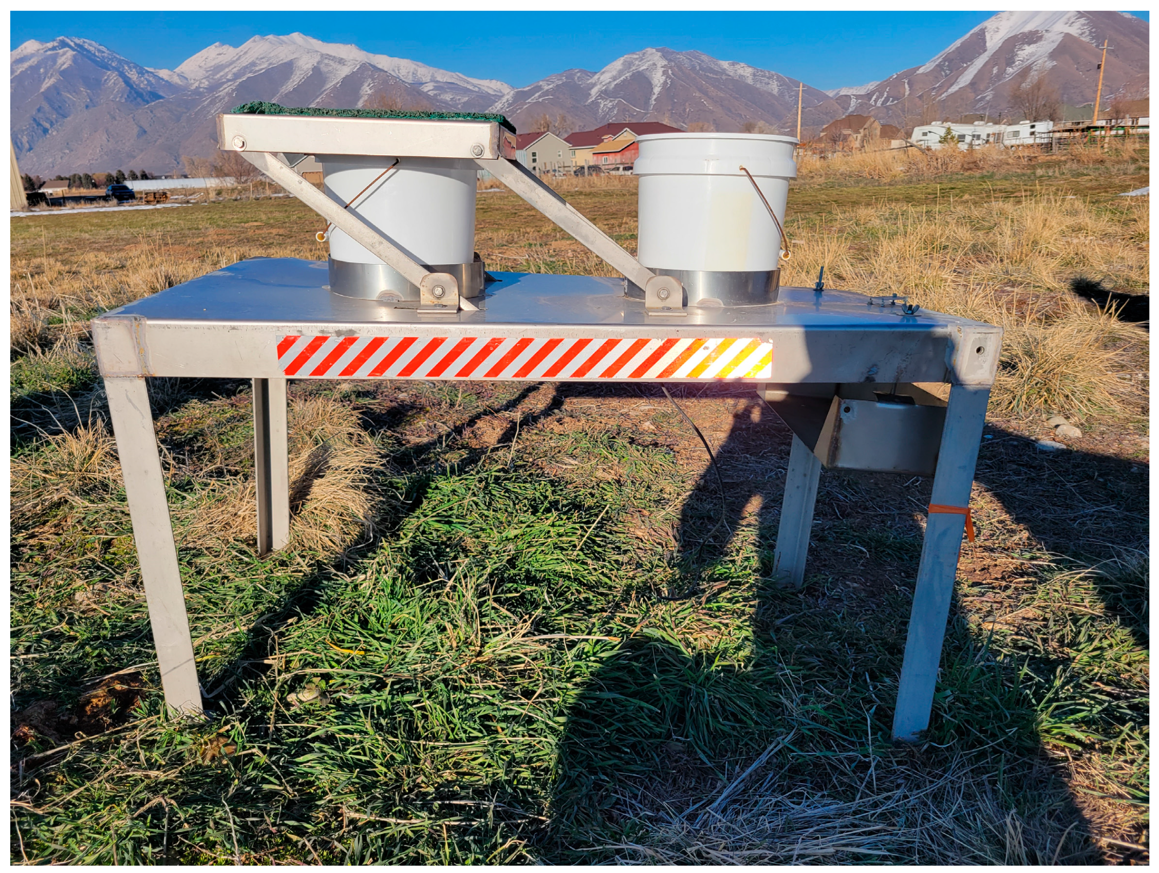
The geologic materials in the deposition samples were obtained from the sample network and design reported by Barrus et al. [36]. This earlier work, and the samples we analyzed here, were designed to quantify total AD to the lake, not to collect dust. For this dust attribution study, we used samples taken at five sites surrounding the lake. The sampler design, seen in Figure 1, consisted of a dry deposition bucket with 3–4 L of water and an empty wet deposition bucket for precipitation with a lid moving to cover one bucket at a time. The dry bucket collects any particulates that contact the water surface, and the wet bucket collects precipitation. Details on sampler placement, design, and operation are provided in [36]. The operation, maintenance, and sampling procedures were performed in accordance with the design of previous studies [27,36].

We collected samples weekly, when possible, from May to October of 2022. Once in the laboratory, we decanted 300–400 mL of liquid collected in the field for nutrient testing, with the remainder stored and later used for this study. After decanting the remaining collected solids in the remaining sample, some solids were likely lost. The wet deposition samples (precipitation events) rarely contained more than 300–400 mL of total liquid. Because this left over sample liquid was not stored, we did not use wet deposition samples for this study, only solids collected in the dry sample buckets. At times, the samplers did not open for precipitation events, and thus, the dry buckets did contain some deposition from precipitation events.

The individual samples did not contain much dust, so we combined individual samples to obtain enough dust to analyze based on season. We combined the weekly samples from May through July into a spring sample and the weekly samples from August through October into a fall sample for each sample location.

Once the samples were combined, we filtered the water using a 0.45 µm cellulose acetate vacuum filter to separate particulates from water to obtain the dust (i.e., solids) for analysis. Traditionally, 0.45 µm is considered the boundary between dissolved and non-dissolved solids in water, so this filtration step separated all suspended solids including colloids [36].

2.2. Prevailing Winds

While smaller dust particles can be transported significant distances at relatively low wind speeds, larger particles require higher wind speeds. In addition, higher wind speeds are required to suspend dust from potential source areas. We expect a significant portion of the dust may be suspended because of mechanical disturbance such as vehicle travel, though we have no data to support this statement, so we discuss only the impacts of wind speed.

We obtained wind data from the Utah Climate data center for 6 different weather stations around Utah Lake [47]. The data consists of 10 min average data for wind speed and direction from 1 January 2017 to 7 July 2022. The data set contains 1.6 million total records. Figure 2 shows five different wind roses from three weather stations located around Utah Lake, selected to demonstrate different wind regimes. The color scale for all the plots is the same. The length of each segment on the roses indicates how frequently the wind blows in that direction (expressed as a percentage of time over the study period), while the color represents the wind speed. The panels, from left to right, show wind roses based on all winds, and winds over 15, 20, 25, and 30 km/h. For panels 2–5, the segment length is scaled to represent percentages only for winds in that speed category rather than the entire study duration. Winds at the Tintic weather station (top row) show that the prevailing wind direction, considering all winds, is from the northeast (left panel); however, for winds over 15 km/h (other panels), it is from the south/southwest. Close examination of the left panel shows these higher winds as small segments, but difficult to see. The middle row, Lincon Point weather station, shows low-speed prevailing winds almost exclusively from the southeast, while higher speed winds are almost exclusively from the southwest. The bottom row, Lindon weather station, shows prevailing winds without a single dominant direction, though nearly all winds over 15 km/h are from the northwest.

These plots show that wind directions for winds over 15, 20, 25, and 30 km/h are similar. Figure 3 shows a map with wind roses for each of the six weather stations. The stations are marked with a small green diamond, with the wind rose for all winds and for winds over 15 km/h located above and below for each diamond, respectively. The color scale is the same as that for Figure 2.

Figure 3 shows that, south of the lake, strong winds are predominantly from the south/southwest, while on the northern portion of the lake, strong winds are predominantly from the northwest. These wind data will help explain the attribution results later in the analysis, and were used to help select potential source sample locations.

2.3. Source and Deposition Samples

Figure 4 shows the location of the five deposition sample locations in light purple, and the 17 potential source sample locations in light red. The deposition sample locations are: Pump Station (northwest corner of lake), Orem (northeast region), Bird Islan (in the lake), Lake Shore (southcentral), and Mosida (southwest). The Lake Shore location is isolated from the Mosida by West Mountain. The 17 potential source locations are, with name and number: 1 = Lake Shore, 2 = Eagle Mountain, 3 = 5-Mile Pass, 4 = Chimney Rock Pass, 5 = Goshen WMA, 6 = Elberta, 7 = Mouth of Spanish Fork Canyon, 8 = Cherry Creek, 9 = Fumarole Butte, 10 = Sunstone Knoll, 11 = Sevier Dry Lake, 12 = Cricket Mountain, 13 = White Hills near Sevier Lake, 14 = Mid-Sevier Lake near road, 15 = Highway 6 South of Delta, 16 = Burraston Ponds, and 17 = Miners Canyon. There is a deposition sample location and a potential source location both named “Lake Shore”, but they are in different locations.

Previous work by Goodman et al. [44] and Carling et al. [43] sampled surface soils from southwestern playa sources near Sevier Dry Lake. We collected our samples representing potential dust source areas (Figure 4) in a larger area. We collected three samples as close as possible to the locations reported in Goodman et al. [44], which are called Sevier Dry Lake, Sunstone Knoll, and Fumarole Butte (Figure 4). We collected additional surface soil samples of potential dust source areas in the open areas between Sevier Dry Lake and Utah Lake (Figure 4), from potential sources areas surrounding the lake, and to the west of the Lake (Figure 4).

We collected soils samples following the EPA AP-42 method, which was used by previous researchers studying surface soils as dust sources [48,49]. We scraped the surface soils with a shovel in an upward direction to a depth of ~2.5 cm (1 inch) or the diameter of the largest particle, whichever was less. As recommended by the EPA method, we collected all the particles in the area and did not avoid large particles. The EPA recommends collecting 10 pounds per site, but we only collected 1–2 pounds to allow for easier storage and transport.

2.4. Sample Preparation and Analysis

We first sieved the potential source soil samples with a 250-µm sieve for 5 min to remove the large particles unlikely to be transported by wind. This sieve size was chosen based on previous particle size analysis performed by Dansie et al. [50], Chepil [51], and Péwé [52], who recommended this size to eliminate particles too large to travel long distances. We did not treat the soil samples to remove organics if the organic material could pass the sieve, as this indicates it was small enough to be transported with the dust. When we collected the Sevier Dry Lake sample it was wet and was allowed to dry over time; this caused the sample to dry into hard clumps that were not easily broken. We broke these clumps apart using a soil flail grinder. Six of the source dust samples were collected when damp and dried in a drying chamber at 45 degrees Celsius overnight. This drying procedure caused some small clumping of the samples; we broke these clumps gently using a clean spatula before sieving.

The previous study filled buckets with 3–4 L of water and collected the water from the buckets weekly to collect dry atmospheric deposition nutrients (and solids) [27,36]. They transported each weekly sample to the laboratory and decanted 300–400 mL of liquid, ~7.5–15% of the sample from the top, and used this liquid to measure nutrient concentrations. Decanting the small sample for nutrient analysis left most of the collected solids in the remaining sample, though some solids were likely lost in the decanting. After decanting, the samples were stored for later analysis. We used these samples to represent deposition to Utah Lake. We only used samples collected from the dry deposition buckets, shown in Figure 1, that had been stored after analysis by the previous study.

We had to discard a few samples that had algae growing in the archived samples, as these would have clogged the filter. We used the remaining archived samples, i.e., the liquid remaining after decanting 300–400 mL for nutrient analysis, to perform source attribution analysis and to quantify mass deposition. For source attribution, this mass loss from either decanting or the few excluded samples is not an issue. Estimates of the mass deposition rates are only approximate as some samples and solids were excluded.

To separate the solids deposited as dust from the water samples, we filtered the sample liquid through 0.45-µm cellulose acetate vacuum filters. We selected this filter type to separate any particles too large to be dissolved and so that the filter material would not affect the nitric acid digestion and ICP-OES analysis. We explored other separation techniques and filter types with little success. The last dust sample collected on 10 October at the Pump Station and had heavy contamination from the seal material on our sampler’s lid. We processed this sample, labeled “Pump Station Contamination” or PS contamination, separately from the other Pump Station samples, rather than including it in the fall sample. However, after analysis, the samples results were not significantly different.

We selected the cellulose acetate filters because they have extremely low-ash content. After filtering the samples to separate the particulate matter, we placed the filters and accompanying solids in a muffle furnace at 500 degrees Celsius for 2.5 h to remove the filter from the samples before digestion [53].

Once the samples were either filtered and reduced to ash (dust samples) or sieved (soil source samples), we digested the resulting samples using a nitric acid microwave digestion method. This digestion method uses 69.9% nitric acid at 170 degrees Celsius for 20 min with 50 min of warmup and cooldown time. As the temperature is above boiling, the digesting is performed in a pressure vessel.

We analyzed the digested samples for element concentrations using a Thermo-Scientific iCAP7400 Radial ICP-OES for 25 elements Al, As, B, Ba, Ca, Cd, Co, Cr, Cu, Fe, K, Mg, Mn, Mo, Na, Ni, P, Pb, S, Se, Si, Sr, Ti, V, and Zn. The results showed that cadmium and selenium were below detection limits for all samples, except for one sample taken at Goshen WMA that had 2 mg/kg selenium. Because of these low concentrations, we removed these elements from the analysis. Thus, we measured 23 elements for each sample. We treated these data as vectors in a 23-dimension sample space. Treating these data as vectors allowed us to compare similarity between samples and potential sources. We computed detection limits according to the EPA method detection limit procedure using the BYU Environmental Analytic Lab soil standard.

2.5. Data Analysis

We used four different methods, two statistical and two visual, to compare the elemental spectral signatures of the dust samples collected near the shore of Utah Lake with soil samples collected in suspected source areas. We used these metrics to determine which source samples were most similar to the deposition samples. The analysis methods were spectral angle (SA) [54], coefficient of determination (R²), and Multidimensional Scaling (MDS) to visualize these two distance measurements [55]. We used multidimensional radar plots to visualize similarities and differences between the samples and potential sources. We computed SA, R², and the radar plots using python. We used SAS JMP Pro version 16 to compute and visualize MDS plots results. The R² value is similar to a Euclidean distance as it is the squared pair-wise difference between two samples normalized by the difference of the sample with the average. While the Euclidean distance is the square route of the squared distances, R² does not apply the square root, but can be thought of as a distance measure in a higher dimensional space.

Figure 5 presents the difference between the two distance measures we used, showing one sample in two-dimensional space (orange) with two potential sources shown in grey and blue for Source A and Source B, respectively. This is analogous to using only 2 of the 23 metals for attribution. The left pane shows that the distance between the two source measurements, and the sample in Euclidian measured using Euclidean distance. In this panel, Source A is much closer to the sample than Source B. In the right panel, we show the SA distance between the sources and samples. In this plot, spectral angle B is much closer to the sample that spectral angle A, indicating that the sample is most likely from Source B. In these plots, if you dilute the sample values with a 1:1 dilution, you obtain Source B, which is closer in chemical composition to the sample than Source A.

SA, rather than measuring the Euclidean distance between two measurement vectors, measures the angle between two measurement vectors in multi-dimensional space [56]:

$$\alpha =arcos\left(\frac{{\sum }_{i=1}^c{x}_i{y}_i}{\sqrt{\sum _{i=1}^c{x}_i^2}\sqrt{\sum _{i=1}^c{y}_i^2}}\right)$$

(1)

where $x_i$ and $y_i$ are the source and measurement data vectors, each with a of length c, which for our data is a value of 23. SA indicates how well the shape of the two series match with an angle of 0, indicating vectors pointing in identical directions. SA is not influenced by differences in magnitude. Spectral angles are the angles created between two vectors in multidimensional space. We created vectors for our samples by assigning each analyzed value a point in an n-dimensional space, where n is the number of values, or 23 for our data. We assume each metal concentration is a separate dimension. The angle between these vectors is then measured, small spectral angles indicate similar samples. Using spectral angles allows us to compare datasets that have similar ratios between the different elements so that concentration or magnitude differences do not interfere. This technique was used to find similarities between geologic samples in previous studies [57]. We used a spectral angle script found in the Hydroerr Python package [58].

MDS is a parameter reduction technique that attempts to preserve pairwise distances from higher dimensions in a lower dimension. We compute a complete pair-wise distance matrix with values for the distance between every set of points. The MDS plot tries to distribute samples such that the Euclidean distance in two-dimensional space between each set of points is proportional to the distance in the higher dimensional space.

MDS allows visualization of similarity between samples, generally using a two-dimensional plot [54]. An MDS plot is interpreted by comparing the proximity of samples in the reduced MDS space where similar samples, those close in higher dimensional space, are placed close together, and dissimilar samples are spread apart. This technique has been used to interpret similarities in geologic samples [59,60]. We evaluated the MDS transform using a Shepard Diagram, which plots the pairwise higher-dimensional distance against the MDS distance for each pair of points. Then, we computed an R² value of the correlation of the MDS distance with the actual distance for both metrics.

We computed MDS plots using both a pair-wise distance matrix, computed using Euclidean distance, and a pair-wise distance matrix, computed using the SA metric. We then used the MDS algorithm to plot these points in two-dimensional space while retaining the proportional distance between each pair of points. We computed distance matrices using phyton with the Hydroerr Package for SA and the Skikitlearn Package for R². We computed the MDS transform values using SAS JMP Pro V16.

Visualizing high-dimensional data is difficult. To show how similar and dissimilar samples are in 23 dimensions, we created radar plots of our data. Radar plots allow for the visualization of the similarities and differences between the samples via the shape of the plot. One feature is that the shapes presented in the plots are not influenced by concentration or magnitude of the data. We used the raw uncorrected ICP data for the radar plots because the dilution-corrected results span a large difference in magnitudes that are difficult to visualize on a single plot without normalizing each measurement. The uncorrected data can be thought of as data normalized for concentrations of each element as we dilute the samples to be within the operating range of the ICP. For these plots, we decreased the uncorrected calcium concentrations by a factor of 12 to fit the radar diagram scale. Soils in this study are calcareous with very high calcium values. With radar plots, magnitude is insignificant; the ratios between elements, and the shape they create, are what are visualized and analyzed. However, if one element is significantly larger than the others, the resulting plot does not show variations in the less concentrated elements well.

3. Results

3.1. Spectral Angle and Coefficient of Determination

We compared each of the deposition sample locations with each of the dust source locations using the spectral angle metric. Figure 6 shows the pair-wise results of the spectral angle analysis as a heat map, with blue, meaning lower angles, being the most similar. Cherry Creek is seen near the top of the map with a dark horizontal line denoting low spectral angles between deposition samples. We found high similarity, low-spectral angles between the Cherry Creek source sample and all the lake deposition sample locations. The Lake Shore deposition site is the least related to the Cherry Creek source. The Chimney Rock source (Figure 4) was next most similar source to all the deposition samples (Figure 6).

The Mosida and Pump Station fall deposition samples were most like the Cherry Creek source material, differing by only 0.34 and 0.35 radians in hyperspace, while the Lake Shore samples, Fall and Spring, were least like the Cherry Creek sources, with spectral angles of 0.79 and 0.67 radians, respectively. Figure 4 shows that based on the geography of the Cherry Creek area, winds from the southwest, which pickup dust from this region, are funneled towards the Mosida sampler, the most correlated in a narrow corridor which opens wider as it enters Utah valley. The Lake Shore location is separated from the Cherry Creek dust source location by West Mountain (Figure 4), which blocks these winds. Cherry Creek is the closest dust source location to the lake.

The Chimney Rock Pass and Elberta sources are similar to all the deposition locations and are subject to wind patterns similar to Cherry Creek. The Eagle Mountain source site is also similar to all the deposition sites. The Eagle Mountain site is located west of the Lake, and it is common to have winds from the west which transport and deposit material from this source. The mouth of Spanish Fork Canyon (S.F. Canyon in the figure) is similar to deposition at most sample locations, as hypothesized.

Figure 7 shows the pair-wise similarity using the coefficient of determination. The color map is reversed so blue represents pairs that are more similar to match Figure 6. These results are comparable to spectral angle results (Figure 6). Again, the most similar source locations are Cherry Creek and Chimney Rock Pass followed by Elberta to the south. Eagle Mountain to the west contributes to all the deposition sample locations.

We can look at each individual deposition location in turn. Mosida and Pump Station Fall samples are most similar to samples from the Cherry Creek and Chimney Rock Pass source locations. The SA measure shows that both spring and fall are essentially the same, while the coefficient of determination measure shows that spring values are slightly less similar to these sites. Mosida in the fall is somewhat similar to six additional source locations: 5-Mile Pass, Burraston Ponds, Eagle Mountain, Elberta, Miners Canyon, and Spanish Fork Canyon, but these similarities are not evident at the Mosida location in the spring. The Orem deposition location is most similar to the Cherry Creek source location, with some similarity to the Chimney Rock Pass source locations, with these similarities stronger in the fall than the spring. Orem is less similar to the other six source locations as Mosida in the fall, though this similarity is less; in the spring, this similarity is not evident. The Lakeshore deposition site is most similar to the Cherry Creek site, with some similarity to the Chimney Rock Pass location. In the fall, it is also somewhat similar to the Lakeshore source location, located near the deposition sampler, though this similarity is lower in the spring. It is not similar to the other source locations. The Pump Station deposition location exhibits behavior like the Mosida location, though similarities are a little lower. Bird Island did not have enough solids to break into two samples, so we only had a single combined sample. It is most similar to the material at the Cheery Creek location, with some similarity to Chimney Rock Pass, it is not similar to any of the other source locations. There was one sample from the Pump Station that was visually contaminated with material from our sampler’s lid seal that was analyzed separately. This sample is most similar to Cherry Creek, but is more similar to all the other sample locations in general—the similarity is more equal.

If we look at the source location, there are eight stations that have little similarity to any of the deposition sites; these are Cricket Mountain, Fumarole Butte, Goshen, Delta, Sevier Lake, Sunstone Knoll, and White Hills near Sevier Lake. Figure 4 shows that, with the exception of Goshen, these are all well to the south, a long distance from the lake. Goshen, while close to the lake, does not have winds that would transport dust as it is isolated by terrain features to the south and east of the location. Eagle Mountain and Five-mile Pass show similarity to all the sites in the fall, with less similarity in the spring, except for the Pump Station deposition location which is near these sources. This fits expectations as winds from the west are common during storm events with winds strong enough to transport solids.

3.2. Multi-Dimensional Scaling Comparison

The MDS results show that several source sample locations cluster closely with the lake deposition locations (Figure 8). The MDS analysis shows a strong similarity between the Cherry Creek and Chimney Rock Pass source locations and all the deposition samples, excluding the Lake Shore deposition samples. The distant playa sources are not grouped with the deposition source samples, although the two Lake Shore deposition samples are closer to several of the playa source samples. Looking wider, the MDS plot shows that source samples obtained west of Utah Lake, including Cherry Creek, Miners Canyon, Elberta, and Chimney Rock Pass, and from the mouth of Spanish Fork Canyon on the east side, are closer to lake deposition samples in the plot. The MDS plot analysis reinforces the results from the SA and R² analysis in Figure 6 and Figure 7.

The MDS plots show that the deposition samples are closer to each than they are to the source samples, which means the deposition samples are more similar to each other than to any source sample (Figure 8). The deposition samples are closer to each other using the R² metric than using the SA metric. Using the SA metric, most of the potential source samples are relatively close to each other.

Figure 8 shows that the two Lake Shore deposition samples are the least similar to local source samples using either distance metric. We attribute this to the fact that the Lake Shore sampler is at the base of the West Mountain on the east side (Figure 4). In this location, West Mountain blocks transport from local sources and the farther playas. The two Lake Shore deposition samples are close to the local source samples to the southwest or to source samples collected directly south of the deposition sampler. We collected the Lake Shore source sample directly south of the Lake Shore deposition location, but samples from these two locations are not close to each other in the MDS plots. This suggests that the main source of deposition to the Lake Shore location is from the southwest, but originating in West Mountain itself or the local agricultural land, neither of which were sampled. The Lake Shore deposition samples are about equal distance from the Lake Shore source location and the Sevier Dry Lake location. This suggests that West Mountain is blocking local transport, but not long-range transport from the distant playas. This is consistent with published results, which showed that Sevier Dry Lake is a dust source for the Utah Valley region [44].

The MDS plots of both error metric, the deposition samples, both fall and spring, from Mosida, Bird Island, and Orem cluster in a group, indicating that these samples are similar to each other (Figure 8). Previous criticisms of deposition research performed by Barrus et al. [36] claimed that deposition should differ between shoreline samples and mid-lake samples. Since these are clustered in the MDS plots, this implies that the source of the material is the same for all three deposition locations. Because Bird Island is in the middle of the lake, while Orem and Mosida are on opposite sides of the lake, this result supports Barrus et al.’s [36] claims of no statistical difference between shoreline to mid-lake atmospheric deposition amounts.

We collected a large number of source location sites around Sevier Dry Lake, which includes Sevier Dry Lake, Mid-Sevier Lake, White Hills, Cricket Mountain, Sunstone Knoll, and Highway 6 (Figure 4). Using either the R² or SA metric, the Sevier Lake sample is not similar to any of these samples (Figure 8). The Sevier Lake sample is from the playa, and, visually, had significant amounts of salts. The other samples are from various different geologic exposures, selected as potential sources; both distance metrics show that the Sevier Lake sample is unique and not similar to either the other potential source samples or the depositoin samples.

To check how well the two-dimensional MDS plots represent the distance metrics computed in 23-demensional space with the distance in the MDS plot, we created a Shepard diagram (Figure 9). A Shepard diagram plots the predicted distance in two-dimensions on the x-axis and with the actual distance in 23-dimension space on the y-axis. Figure 9 shows that the predicted distance in two-dimensions is very well correlated with the actual distance in 23-dimensions, with an R² value of 0.993.

3.3. Visual Comparison

Radar plots present muti-dimensional data in an easily interpreted form with each element plotted on radial lines. The shape of the plot presents the concentration ratios among the various elements. These shapes are invariant with dilution or concentration, but clearly show variations in relative concentrations among the elements. Figure 10 shows that the Cherry Creek source sample has a shape that is visually similar to both the Mosida fall and Orem fall deposition samples, but different from the Sevier Dry Lake source sample. Figure 10 shows that the main shape difference between the Cherry Creek source sample and the lake deposition samples is the high silica and calcium concentrations in the Cherry Creek sample. We attribute this to sample preparation, where the Cherry Creek sample had larger sand and limestone particles which would increase silica and calcium concentrations, which were not transported and captured in the deposition samples. To test this hypothesis, we sieved the Cherry Creek sample with a 150-µm screen, but found no major difference in the shape. We did not attempt to sieve the sample for smaller sizes, which could more easily be transported by wind. A 150-µm sample would only be transported under high winds and for short distances [8,61]. The similar shapes of the Mosida and Orem deposition samples indicated that dust sources are likely the same, supporting the claims that dust deposition across the lake does not change significantly.

4. Discussion

As discussed in Section 2.1, the samples we used for this analysis were not designed to quantify the amount of solids in atmospheric deposition to Utah Lake, rather they were designed to measure nutrient deposition [36]. To obtain a rough estimate of the mass deposition rate, we used weekly samples collected from the previous study collected over 6 months from May to October 2022. We discarded some samples (Section 2.1).

For source attribution we needed a large enough mass of the deposited solids for ICP analysis, about 0.03–0.04 g (i.e., 30–40 mg). Solids deposition rates at Utah Lake are so low that we needed to combine the individual weekly samples from any given deposition location to obtain enough dust to analyze. We combined the weekly samples into two seasonal samples, with samples from May through July combined into a spring sample and samples from August through October combined into a fall sample. This was performed for each sample location. The resulting composite samples consisted of the solids from about 12 weekly samples. At the Bird Island deposition location, we combined all the weekly samples into a single composite sample because the total mass was too low for analysis if split. One sample at the Pump Station deposition location was visibly contaminated so we did not combine this sample with the others but analyzed it separately.

As discussed in Section 2.1, we filtered the samples on 0.45 µm filters, then dried the filters to measure the mass of solids in each sample; 0.45 µm is considered the dividing line between dissolved and suspended solids, so this preparation method captured all the suspended solids. The filters were then reduced to ash and dissolved for analysis.

The resulting data (

Table 1. Weights of dust collected over the course of 5.5 months for this study.

Location	Spring (g)	Fall (g)	Total (g)
Mosida	0.07	0.05	0.12
Lake Shore	0.11	0.11	0.22
Pump Station	0.16	0.03	0.19
Orem	0.07	0.05	0.12
Bird Island			0.05
Pump Station (Contaminated)			0.04

) show that over the 6-month collection period, the total mass collected at any given location ranged from 50 mg to 220 mg at Bird Island and Lake Shore, respectively. The buckets have a surface area of 0.0615 m² [27,36] and Utah Lake has a surface area of approximately 40,000 ha (95,000 acres), which gives a total deposition mass over the 6-month period of about 325 to 1400 kg [42]. This is a unit deposition rate of 0.8 g/m² to 3.6 g/m² over the 6-month sample period for Bird Island and Lake Shore, respectively.

Brahney [8] reported dust deposition in Provo from 28 to 49 g/m²/yr, significantly higher than our values. We attribute this to our shorter sampling period and the fact that we excluded any precipitation samples. Brown et al. [42] found that about 50% of phosphorous deposition is related to precipitation. We did not capture any dust deposited during the winter months and we also excluded some samples.

While the samples we analyzed were not collected to measure the mass of dust falling on the lake, we did collect and weigh all solids greater than 0.45 µm in the archived samples (Table 1). These results indicate that the mass of solids greater than 0.45 µm deposited on Utah Lake is low, as are the corresponding estimated mass deposition rates.

Our estimates of mass deposition are not truly representative of the amount falling on the lake, but provide good order-of-magnitude data. The few discarded samples and decanted liquid are unlikely to have changed the mass estimates significantly. Members of the Utah Lake Science Panel have argued that the main source of nutrient loading to Utah Lake is dust [8]. They assumed that the dust had nutrient levels similar to those measured in Utah Lake sediments [26,35] and showed that if these concentrations were correct, then it would require unreasonable dust deposition to match the nutrient loadings calculated by Barrus et al. [36]. Our data show that neither dust is the primary vehicle for atmospheric deposition of phosphorous to Utah Lake, or that the small particles, less than 10–20 µm, can have significantly higher phosphorous concentrations. This is supported by the literature, which shows that phosphorous readily sorbs onto small particles.

This level of mass deposition strongly suggests that dust is not the primary source of nutrient loading to Utah Lake, as estimated phosphorous nutrient loads range from as low as 150 to 200 Mg per year [27,36,42]. These mass dust measurements support the research by Brahney [8], who estimated about 15 Mg/yr of phosphorus when considering solid particulates alone, whereas the Utah Lake Science Panel estimated 30 Mg/yr [62]. Brown et al. [42] measured about 120 Mg/yr from precipitation. Barrus et al. [36] measured about 230 Mg/yr from all sources. This implies that deposition from dust is about 6.5% to 13% of total phosphorus deposition, precipitation is about 52%, and dry or contact deposition ranges from 35% to 41.5% of the total.

This is likely due to dust deposition consisting of larger settleable particulates compared to bulk deposition, which includes dry or contact processes, containing particulates that do not settle. Bulk deposition is able to wash the PM2.5 fraction during precipitation events, and these small particles contain higher phosphorus levels [24] than larger particles. The period of this study was during high-dust production for the area; in the months before and after the study, the area is often wet or snowy, preventing local dust generation. While we have no data, we do not expect significant solid mass deposition during the winter and spring months, i.e., November through April.

The dust weights provide insight into spatial dust deposition across the lake. The Orem and Mosida samplers are on opposite sides of the lake and collected nearly identical amounts of dust. The MDS plot in Figure 8 shows that dust collected at the Orem and Mosida samplers are similar and plot close to each other in MDS space. The similar weight and composition of the two samples suggests that deposition does not change significantly across the lake. The Bird Island sampler collected far less dust. Several Bird Island samples showed zero or near zero dust collected for the week, while a single sample in the last week of collection more than doubled the total dust collected at this site. This might be caused by Bird Island’s proximity to West Mountain. It is possible that the mountain is channeling the winds in a way that misses Bird Island while still crossing from Mosida to Orem. However, as shown by Barrus et al. [36], nutrient deposition at Bird Island is not statistically different from deposition at the other stations. Our data show that dust deposition is different. We attribute this to the fact that dust deposition is likely less than 15% of total deposition. Also, large particles make up the bulk of the mass for dust deposition, but have a lower associated nutrient concentration [24]. This supports the conclusion that nutrient deposition does not fall off across the lake, while dust deposition does.

While this study focused on Utah Lake dust attribution, the methods and approach presented here can be applied to many situations involving source attribution for particulate matter such as dust or sediments. Published dust source attribution studies often use methods such as strontium isotopes [43,63], atmospheric transport modeling [16], advanced spectroscopy methods [64,65], X-ray diffraction [65], and X-ray fluorescence [66]. In their introduction, Zhang et al. [66] provide a broad overview of methods used for dust attribution that includes additional methods. Our approach, using ICP analysis, generally requires a simpler sample preparation and analysis approach that can be cost effective compared to these more advanced geochemical methods. We showed that this approach is sensitive and clearly differentiates soil particles from different sources. The MDS plots clearly group locations from similar geologic formations together and match our understanding of atmospheric transport. The methods presented in this study can be used for dust, soil, and sediment attribution in an easy, cost-effective manner.

5. Conclusions

Our data show that most of the dust deposition on Utah Lake comes from local fields south and west of the lake. Both MDS distances and Spectral Angle analysis show that the Cherry Creek source location is most similar to all the deposition locations, closely followed by the Chimney Rock Pass source location. The more distant desert playa sources likely still contribute to deposition, but contribute less than local areas. The two Lake Shore samplers, both source and deposition, are less similar to the other local sources and show the strongest similarity to the desert playas. This is likely due to the sampler’s proximity to West Mountain, which blocks local transport from Cherry Creek, but not long-range transport from the desert playas. While these two sample locations are closer to the playa sources than the other deposition locations, they do not plot closely and are most similar to each other.

Dust deposition is likely a minor source of the nutrient loading onto Utah Lake. This was shown by the research of Brahney [8], who evaluated dust deposition in the literature and found small nutrient loads compared to Brown et al. [42] and Barrus et al. [36] who measured deposition using different methods at locations around the lake. We see evidence that dust is a minor contributor to nutrient loads when the dust weights at Bird Island are lower than the shore locations, but nutrient loadings at Bird Island are not statistically different from shore locations [36]. Large dust particles cannot be the main source of nitrogen and phosphorus when small amounts of dust were collected, but nutrients were still present. We attribute this to much higher nutrient concentrations on small, PM10 and PM2.5 size particles [24].

Dust deposition sources around Utah Lake appear to be relatively similar with similar deposition rates, as evidenced by the similarity between the Orem and Mosida deposition samples, which are most similar to the Cherry Creek and Chimney Rock Pass source locations. The near identical dust weights and similar source compositions suggest that the dust concentrations are not changing across the lake. The Bird Island sampler is located just south of the path between Orem and Mosida and collected similar dust compositions but far less dust. This may be due to Bird Island’s proximity to West Mountain, which may affect wind patterns and shield the island to some degree.

While this study focuses on source attribution for Utah Lake, we present methods and data that can be used for dust attribution in any setting. ICP data are relatively inexpensive and easy to obtain. They are precise and provide good fingerprints for attribution. The use of MDS and Radar plots simplifies attribution analysis, both visually showing both proximity in high-dimensional space. MDS plots provide analysts with clear metrics for attribution. We demonstrated MDS plots with two distance metrics, Euclidean distance and SA, but MDS plots can be used for any other error metric between two measurements with many parameters, such as R². Data from other sources can also be used in MDS plots, as long as the data are normalized so that the various parameters have similar magnitudes.

We present this study to both further the understanding of dust sources to Utah Lake and provide a method for soil and dust attribution. We encourage others to use and extend these tools. We showed that this approach is sensitive and clearly differentiates soil particles from different sources. The methods presented in this study can be used for dust, soil, and sediment attribution in an easy, cost-effective manner.