Abstract
The interaction between soil moisture (SM) and evaporative fraction (EF), which reflects the degree of exchange of water and energy between the land and the atmosphere, is an important component of the theory of land–atmosphere coupling. Exploring the relationship between SM and EF in the transitional climate zone of China can help deepen our understanding of the characteristics of water and energy exchange in this region of strong land–atmosphere coupling. Data on observations in fluxes in the transitional climate zone revealed that fluxes in the energy on the surface of the land in this region exhibited significant inter-annual variations. The sensible heat flux (SH) exhibited the largest fluctuations in July and August, while the latent heat flux (LE) varied the most from June to August. The EF was found to exhibit weak correlations with indicators of vegetation growth such as the leaf area index, Normalized Difference Vegetation Index, and gross primary productivity in the transitional zone of the East Asian summer monsoon. By contrast, the relationship of land–atmosphere coupling between EF and SM in the transitional climate zone was stronger. Based on an analysis of the consistency of the relationship of SM-EF coupling, when the SMP reached 35%, there was a significant transition in the linear relationship between the SMP and EF that was consistent between the shallower and deeper layers of soil (0–40 and 40–80 cm). However, neither level had SM that reached saturation during the six-year observational period (2007–2012), and the mean values of its probability density function showed that the deep soil was drier than the shallow soil. This characteristic shows that SM plays a dominant role in variations in the EF in the transitional climate zone, which in turn indicates that constraints on the moisture govern the SM–EF relationship. The results of this study provide a better understanding of the mechanisms of land–atmosphere coupling in the transitional climate zone of China.
1. Introduction
The interactions between the land surface energy and the water and carbon cycles profoundly influence the evolution of various layers in the Earth’s climatic system. Evapotranspiration plays an important role in the exchange of energy between the surface of land and the atmosphere. More than half of the net radiation (Rn) absorbed by the Earth’s surface is consumed by evapotranspiration (ET) [1], and approximately 60% of it is returned to the atmosphere [2].
Given the significant role of evapotranspiration in land–atmosphere coupling, establishing universal relationships between evapotranspiration and other factors to reflect land–atmosphere interactions has become a crucial objective in the field of land–atmosphere coupling. Drawing on the conceptual model proposed by Budyko et al. [3] and incorporating the findings from Koster et al. [4], Seneviratne et al. [5], and Teuling et al. [6], Seneviratne et al. [7] categorized the dominant factors controlling evapotranspiration into three types based on the quantitative relationship between evaporative fraction and soil moisture: A soil moisture-limited region, an energy-limited region, and a region with joint energy and soil moisture limitations.
Large variations in the soil moisture (SM) and ET in zones of climate transition can lead to the transfer of moisture and energy to the upper atmosphere through the exchange of water vapor and energy. This results in a weakening of atmospheric stability and an increase in atmospheric disturbances, because of which zones of climate transition are regions featuring strong land–atmosphere coupling [8]. For example, the climate transition zones in the North American Great Plains, the Sahara region, Equatorial Africa, and Asia are all global hotspots for land–atmosphere coupling [4]. The strength of the coupling between ET and the atmosphere is three times that of the coupling between the SM and the atmosphere in the climate transition zone in the Great Plains of the southern United States [9], and this leads to frequent and severe weather events in the region. The climate transition zone in China is not only the region with the highest variations in ET but also serves as a semi-arid zone of transition in which the humid climate of the southeast transitions into the arid climate of the northwest [8]. It is also a zone of ecological transition from broadleaf forests to grasslands and deserts [10]. Previous research has shown that some weather-related and climatic phenomena in the zones of climate transition are significantly different from those in other climatic regions. Zhang et al. [11] reported a significant increase in pan evaporation in the Chinese climate transition zone over the past 50 years, where this is opposite to the “evaporation paradox” commonly observed in other regions of the world and constitutes the unique “anti-evaporation paradox”. The thickness of the stable boundary layer, height of the residual layer, and thickness of the convective boundary layer all exhibit stepwise reductions from the non-monsoon regions to the transition zone and continue to decrease stepwise to the monsoon regions [12]. Zhang et al. [13] showed that a reversal occurs in the relationship between ET and other environmental factors when the SM, wind speed, Rn, and Normalized Difference Vegetation Index (NDVI) reach certain thresholds.
As a key factor in land–atmosphere coupling, ET is often described using complex mathematical relationships to capture the influence of the environment and the climate [14] and involves a certain degree of uncertainty [15]. Research has shown that the evaporative fraction (EF, defined as the latent heat flux normalized by latent plus sensible heat flux) can more clearly depict the constraining relationship between the process of ET and other elements in different climate zones than ET itself.
When values of the daily Rn exceed their average level in the climate transition zone in the southern Great Plains of North America, the EF exhibits a linear correlation with the SM, and the relationship of coupling between them shows significant interannual differences [16]. The slope of this relationship is more strongly correlated with the status of growth of the underlying surface vegetation under the influence of other meteorological conditions, which is often a non-linear relationship [17]. Zhang et al. [18] used sensitivity experiments on the parameters of the land surface to quantitatively estimate land–atmosphere interactions by using the relationship between the EF and the SM. The results showed that changes in the SM in the climate transition zone can lead to average variations of 1.1–1.3 K in the surface temperature (Ta) that can reach 6–7 K [19]. This parametric relationship provides theoretical support for modeling SM–EF interactions. Basara and Crawford [20] identified a strong linear correlation between the SM and the surface energy that represents strong land–atmosphere coupling under ideal weather conditions (i.e., clear skies, low winds, and no recent precipitation). Chen et al. [21] identified a third-order relationship of polynomial fit between the SM and the EF in the Qinghai–Tibet Plateau to confirm the strong EF-SM coupling in high-altitude regions. Studies have also shown that when the leaf area index (LAI) is used instead of the SM, the strength of EF-LAI coupling is three times that of EF–SM coupling. The gross primary production (GPP) is also strongly coupled with the EF when the underlying surface contains crops [9]. It is thus clear that the EF exhibits strong characteristics of coupling with the SM, LAI, and GPP in climate transition zones, where the coupling relationship and its strength vary owing to regional climatic and elemental environmental differences. However, research on the relationship between the SM and EF in China’s climate transition zone remains inadequate, such that the relationships between the LAI and EF and the GPP and EF remain unclear. To fill this gap in research, the authors of this study used a dataset based on environmental observations from the Lanzhou University (SACOL) station, which is located in a region with a semi-arid climate, to investigate the relationships between the SM and EF, the LAI and EF, and the GPP and EF in the climate transition zone of China.
2. Materials and Methods
2.1. Site and Dataset Descriptions
A comprehensive and continuous set of in situ measurements of flux is crucial for research on land–atmosphere interactions. The SACOL (shown in Figure 1) is among the few stations for the long-term and continuous measurements of flux in land–atmosphere interactions in the transitional zone of China’s summer monsoon. The reliability of data provided by the SACOL has proven to be instrumental for research on the surface energy and water and carbon cycles over transition zones [22,23,24].
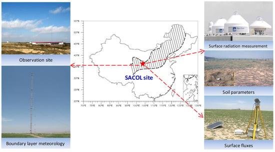
Figure 1.
Map and photographs of the SACOL station. The star in the middle represents the location of the SACOL station, and the shaded area represents the transitional climate zone in China. The two figures on the left show the observation field and the gradient tower, while the three figures on the right show observations of the surface radiation, parameters of the soil, and surface fluxes.
The SACOL station is located in the western part of China’s transitional climate zone (35°57′ N, 104°08′ E), with an elevation of 1965.8 m. The mean annual volume of rainfall and Ta are 386.5 mm and 7.4 °C, respectively [25]. More than 80% of the annual precipitation occurs in the growing season [13], while desert grasslands constitute the dominant vegetation on the land surface. The growing season is the period of the year when crops and other plants grow successfully. The growing season dates in a region are closely related to the climate. In China’s transition climate zones, the growing season typically spans from early April to the end of September [13].
An eddy covariance (EC) system was installed at SACOL that consisted of a three-dimensional (3D) sonic anemometer (CSAT3, Campbell Scientific, Salt Lake, UT, USA) and an open-path infrared gas analyzer (LI7500, LI-COR, Lincoln, RI, USA). The sonic anemometer was used to measure the 3D wind speed and the virtual temperature. The open-path infrared gas analyzer provided simultaneous measurements of the concentrations of water vapor and carbon dioxide. Boundary layer meteorological measurements were used to record the wind speed (014A-L, Met One, Salt Lake, UT, USA), the Ta of air, and the relative humidity (HMP45C-L, Vaisala, Helsinki, Finland) at heights of 1, 2, 4, 8, 16, and 32 m. The upward and downward shortwave radiations were measured using CM21 radiometers (Kipp & Zonen, Delft, The Netherlands), while the upward and downward longwave radiations were measured using CG4 radiometers (Kipp & Zonen, Delft, The Netherlands). The volumetric water content of the soil was collected by using CS616 (Campbell Scientific) at depths of 5, 10, 20, 50, and 80 cm. In addition, reliable methods were used to control the quality of the data, as well as the annual calibration of the instruments. Linear interpolation and Falge’s method [26] were used to enhance the reliability of the dataset [24]. Each time series was screened for spikes, and the discarded values were interpolated. Spikes are defined as points exceeding 4.0 times the standard deviation in a 60-s window. If spikes and unrealistic values surpassed 1% of the total data points, the entire run was discarded. Incomplete records (<5 min) were removed. The results indicate that spikes insignificantly impact turbulent flux measurements. Variances and covariances were computed through 30 min block-averaging. Addressing potential time delays, cross-correlation analysis corrected for sensor separation, and lag-time bounds were set at 1.0 s for each interval. Then, a series of tests were conducted to check the reliability of the data [24]. A specific QA/QC system, including data post-processing and quality control, was developed for SACOL. The procedure of post-processing included time delay correction, coordinate rotation, frequency response corrections, sonic temperature correction, and WPL correction. The procedure of quality control included the test for physically not possible values and spikes, the stationarity test, and the integral turbulence characteristics (ITC) test [24]. Furthermore, all of the instruments installed at the SACOL site were calibrated every year in order to ensure the reliability and continuity of the dataset [13]. More details regarding the profile of the SACOL station and the in situ measurements have been provided by Zuo et al. [24] and Liu et al. [23].
The NDVI was derived from the MOD09GA version 6.0 product and had passed phase 3 verification (https://doi.org/10.5067/MODIS/MOD09GA.006, (accessed on 20 June 2023). The gross primary productivity (GPP) represents the growth of the terrestrial vegetation and was derived from the Global OCO-2 based SIF product (GOSIF). This is a new global product of solar-induced chlorophyll fluorescence [27]. The LAI was derived from the MOD15A2H version 6.1 moderate-resolution imaging spectroradiometer (MODIS). The dataset consisted of eight-day composite data with a pixel size of 500 m (https://lpdaac.usgs.gov/products/mod15a2hv061/, (accessed on 20 June 2023).
Using the MODIS L1B as the primary input and performing corrections for the effect of gaseous absorption, molecules and aerosol scattering, coupling between atmospheric and surface bidirectional reflectance function (BRDF) and adjacency effect (atmospheric point spread function), surface reflectance was produced for high-level NDVI and LAI. NDVI (Level2G) and LAI (level 4) were radiometrically calibrated and atmospherically corrected [28].
2.2. Methods
The daily surface (mm day−1) was calculated as follows [29]:
where is the latent heat flux (MJ m−2 day−1), is the latent heat of vaporization of water (2.45 kJ g−1), and is the density of water (1 g cm−3). The evapotranspiration rate expresses the amount of water lost from land surface in units of water depth. Water depths can be expressed in terms of energy received per unit area. Formula (1) facilitates the conversion between the observed latent heat flux and water depth.
The was calculated as follows [9]:
where is the sensible heat flux (MJ m−2 day−1). The varied from zero to one and can reflect the land–atmosphere coupling in a region by characterizing the partitioning of net radiation among surface energy fluxes.
The soil moisture percentile was calculated as follows [30]:
or
where is the percentile, is the lower bound of the array containing , is the upper bound of the array containing , is the frequency of within the array, stands for the cumulative frequency below , represents the cumulative frequency above , and is the interval width [30]. In this study, percentiles were used to analyze the statistical characteristics of the soil moisture.
3. Results
Variations in Climatic Elements
The strength of land–atmosphere coupling in a climate region is closely linked to both the patterns of atmospheric circulation and the magnitude of the surface energy fluxes and the SM. The Bowen ratio (BR) is an important parameter representing the proportions of energy allocation and provides information on surface dryness or wetness. Understanding the statistical characteristics of the land surface and atmospheric climatic elements contribute to our understanding of the climatic background of land–atmosphere coupling in the study region.
Table 1 presents the statistical values of Ta, major surface energy fluxes, shallow and deep SM, EF, and BR recorded at the SACOL site during the seasons of vegetation growth (April–September) from 2007 to 2012. The average Ta during the growing season was 15.8 °C, with a daily average variance of 4.7 °C. The mean values of the SH, LE, and Rn were 42.2, 47.4, and 103.8 W m−2, respectively, with daily average variances of 23.2, 24.6, and 44.7 W m−2, respectively. It is evident that large fluctuations in the daily surface energy fluxes were the main reason for the large daily variations in Ta in the transitional climate zone. The annual average values of the SM in a depth range of 0–40 cm varied by a range of 0.109 to 0.153 m3 m−3, with a daily average variance of 0.038 m3 m−3. The annual average values of the SM varied from 0.092 to 0.148 m3 m−3 in a depth range of 40–80 cm, with a daily average variance of 0.032 m3 m−3. This indicates that the values of the SM and the amplitude of fluctuations in the deeper layer (40–80 cm) were smaller than those in the shallower layer (0–40 cm) in the transitional climate zone. The mean values of the BR during the growing season fluctuated between 1.22 and 2.27, with a daily mean variance of 1.66, while those of the EF ranged from 0.36 to 0.56, with a daily mean variance of 0.20 (Table 1).

Table 1.
Statistical information of the elements of land–atmosphere coupling in the growing season from 2007 to 2012.
The surface heat flux is transported upward to the atmosphere through turbulent processes and has a direct feedback effect on the atmosphere. Changes in the surface heat flux, regardless of whether it increased or decreased, had a direct impact on the state of the atmosphere. This is a key component of the process of land–atmosphere coupling and plays a determining role in the coupling between the ET and the SM.
Figure 2 shows the analysis of the variations in the Ta, Rn, and surface heat flux during the growing season from 2007 to 2012. The six-year averages show that the SH in the transitional climate zone generally exhibited a fluctuating trend of decrease in the growing season (April to September) (Figure 2a). The LE gradually increased, reaching its maximum from late August to early September, and then gradually decreased (Figure 2b). The variations in the Rn and Ta were relatively consistent, and both showed an increase to their maximum values in late July to early August, followed by a gradual decrease (Figure 2c,d). The interannual fluctuations in the Rn and SH were most pronounced in July, with values of 47.3 and 15.0 W m−2, respectively. The interannual fluctuation in the LE was most pronounced in July, with a value of 45.7 W m−2. This indicates that significant interannual variations in precipitation in the transitional climate zone in July induce substantial differences in the surface moisture necessary for the latent heat process. Consequently, this impacts latent heat flux and exerts a significant influence on it [13].
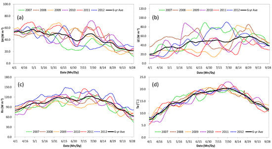
Figure 2.
Variations in the (a) SH, (b) LE, (c) Rn, and (d) Ta of air from April to September. All of the data represent the 21−point moving average of the daily values from 2007 to 2012.
The seasonal variations in the SM in the transitional climate zone in the depth range of 0–40 cm revealed distinct patterns. The average annual SM gradually decreased before mid−May and began to gradually increase from then on (Figure 3a). This reflects the characteristics of increased atmospheric precipitation and significant interannual differences in the transitional climate zone beginning in mid−May. An examination of the trends of the NDVI makes it clear that with the rising temperatures starting from April, the NDVI exhibited a gradual and fluctuating increase to reach its peak value in late August, followed by a gradual decline (Figure 3b). By contrast, values of the BR and EF exhibited opposite trends (Figure 3c,d). Specifically, the BR decreased during the growing season while the EF increased, once again highlighting the combined impact of the increasing SH and the decreasing LE on the distribution of surface energy fluxes. Furthermore, the SM, NDVI, BR, and EF all exhibited significant interannual fluctuations, demonstrating the pronounced interannual differences in land–atmosphere coupling in the transitional climate zone.
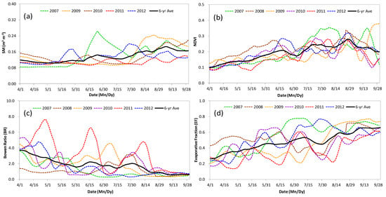
Figure 3.
Variations in the (a) SM at 0–40 cm, (b) NDVI, (c) BR, and (d) EF in the growing season from April to September. All of the data are the 21−point moving average of the daily values from 2007 to 2012.
The surface energy, water, and processes of carbon exchange are crucial components in the process of coupling between the land surface and the atmosphere. The process of carbon exchange is directly influenced by the levels of activity of the first two processes and is closely related to conditions of the surface vegetation, as reflected by the LAI and NDVI [31]. Bagley et al. [32] found that prior to the harvest season in the southern Great Plains of the United States, the EF was highly coupled with the LAI of winter wheat. However, the EF exhibited a higher correlation with the SM after harvest. Williams et al. [9] also researched the southern Great Plains region of the United States and discovered that the EF had a sound non−linear correlation with the LAI in grasslands and a good linear correlation with the LAI and GPP in areas with crops, with R−squared values of 0.53 and 0.67, respectively. Moreover, the correlation between the EF and the SM in the case of different underlying surfaces was not consistent.
Figure 4 depicts the relationships between the EF and the SM and indices representing the conditions of vegetation (GPP, LAI, and NDVI) in the transitional climate zone of China. It shows that there was no significant correlation between the EF and the LAI or the NDVI, with linear correlation coefficients (R−squared) of 0.11 and 0.02, respectively (Figure 4a,b). Figure 4b,c does not pass the significance test at the 95% confidence level. Although a higher correlation was observed between the EF and the GPP, with an R−squared value of 0.37 and a confidence level of 95%, it was not very strong (Figure 4c). A further examination of the relationship of distribution between the EF and the SM reveals that the former exhibited relatively consistent patterns of distribution with the latter in both the 0–40 and 40–80 cm layers of soil, suggesting some level of coupling between them (Figure 4d,e). It is evident that the correlations between the EF and the LAI, NDVI, and GPP were weak in the transitional zone of the Chinese summer monsoon, indicating a significantly lower degree of coupling compared with that in the southern Great Plains of the United States [9].
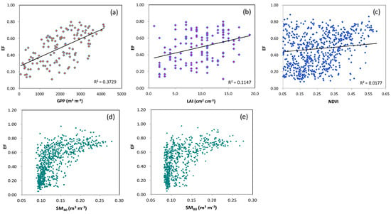
Figure 4.
Responses of the evaporative fraction (EF) to variations in the (a) gross primary productivity (GPP), (b) leaf area index (LAI), (c) Normalized Difference Vegetation Index (NDVI), (d) SM at 0–40 cm (SM40), and (e) SM at 40–80 cm (SM80) in the growing season in the transitional climate zone in China. All of the data are the daily values from 2007 to 2012.
Examining the relationship between the distributions of the EF and SM in different layers in the transitional climate zone of China revealed distinct and regular patterns. The EF had a cubic fitting relationship with the SM in all layers (0–80 cm), similar to the relation of the EF−SM distribution observed in the Qinghai–Tibet Plateau [21]. By comparison, the EF had a higher correlation with the SM in layers in the range of depth of 0–40 cm, with the fitting coefficients of the cubic distribution ranging from 100 to 200. The coefficients of the fitting of the cubic distribution of the EF and SM ranged from 200 to 300 in layers at depths of 40–60 and 60–80 cm, respectively, indicating a more consistent distribution of the correlation in these layers. Therefore, it is useful to study the SM in the transitional climate zone in two distinct layers, 0–40 and 40–80 cm, to better analyze the coupling relationship between the EF and SM.
In addition to directly exploring the fitting relationship between the EF and SM, as shown in Figure 5, Ford et al. [16] discovered that the EF exhibits certain regularities in its pattern of distribution with a sequence of soil moisture percentiles (SMPs). They segmented the relationship between the EF and SM into two stages based on the SMP. For example, the coupling relationship between the EF and SMP was found to undergo significant changes when the latter approached a critical value of around 30% in the southern Great Plains of the United States [16]. The above analysis shows that the critical value of the SMP in the transitional climate zone of China was close to 35% in both the 0–40 cm layer and the 40–80 cm layer (Figure 6). Figure 6 shows that while the EF increased with the SMP in the 0–40 cm layer, there were significant differences between their trends of growth. The EF exhibited a trend of decrease in the 40–80 cm layer, with an initial increase in the SMP followed by a reduction. A comparison with the original data shows that a sufficient amount of precipitation during the growing season led to a replenishment of the SM. The EF then gradually increased due to evaporation, leading to a gradual loss of the SM and a decrease in the SMP. This decrease in the latter intersected with values of the EF at or near the 35% percentile, indicating a change in their relationship.
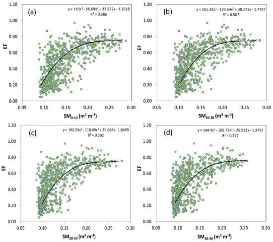
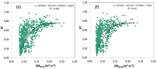
Figure 5.
Responses of the EF to variations in the SM at (a) 0–10 cm (SM0–10), (b) 10–20 cm (SM10–20), (c) 20–30 cm (SM20–30), (d) 30–40 cm (SM30–40), (e) 40–60 cm (SM40–60), and (f) 60–80 cm (SM60–80) in the growing season over the transitional climate zone in China. All of the data are the daily values from 2007 to 2012.
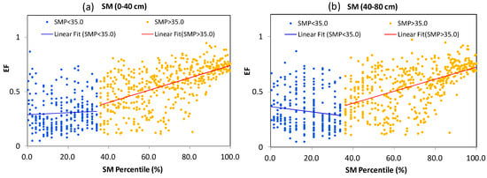
Figure 6.
Responses of the EF to changes in the SMP at (a) 0–40 cm and (b) 40–80 cm in the growing season over the transitional climate zone in China.
The EF–SM relationships over the study period also showed a turning point in the coupling relationship between the EF and the SMP when the latter reached 35%. The analysis of the relationship between the EF and SMP in the 0–40 cm layer (Figure 7a) shows that the former increased with the latter when it was less than 35% (except in 2011). This indicates that when the SM in the transitional climate zone had been replenished, a rapid loss of the SM occurred in the 0–40 cm layer, owing to strong solar radiation, and led to a decline in the EF with an increasing SMP. This trend was more pronounced in the wetter years of 2007 and 2012 [13]. By contrast, the limited replenishment of the SM due to precipitation, coupled with a high Rn on the surface, led to a rapid loss of the SM in the severely dry year of 2011, with an initial increase in evaporation followed by a decrease. When the SMP exceeded 35%, the EF consistently increased with the SM, reflecting the typical characteristics of evaporation being dominated by the SM [7].
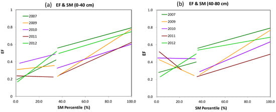
Figure 7.
Responses of the EF to changes in the SMP at (a) 0–40 cm and (b) 40–80 cm in the growing season from 2007 to 2012 (excluding 2008) over the transitional climate zone in China.
When the SMP was less than 35%, the EF decreased with increasing SMP in the 40–80 cm layer in all years except for the unusually wet years of 2007 and 2012 (Figure 7b). This shows that after the replenishment of the surface SM, the surface EF increased rapidly in the dry years. However, due to a lag in the replenishment of the deep SM [31], the values of the latter remained relatively low, even after an increase in the surface SM. When the deep SM was eventually replenished and its value increased, the loss of water from the shallow soil due to evaporation led to a decrease in evaporation and the EF. This led to a reduction in the EF with an increasing SMP in the 40–80 cm layer (Figure 7b). When the SMP was less than 35%, the surface SM was relatively high and stable, and the rate of water loss was closely related to evaporation. Therefore, the EF and the SMP were positively correlated in this scenario.
It is clear from the above analysis that the SM was the dominant factor controlling the EF in the transitional zone during the summer monsoon. We thus needed to better understand the overall characteristics of the distribution of the SM in this zone. The probability distributions of the SM in the dry and wet years (Figure 8) show that both the shallow and the deep SM exhibited skewed distributions overall, with coefficients of skewness of 1.75 in the dry years, 0.84 in the wet years, and 1.19 during the entire observational period. The average values of the shallow SM in the dry years, wet years, and the entire observational period were 0.124, 0.142, and 0.134 m3 m−3, respectively. Its average values in the dry and wet years exhibited symmetric distributions during the entire observational period in the 0–40 cm layer. However, the coefficients of skewness of the SM in the dry years, wet years, and the entire observational period were 1.97, 0.99, and 1.39, respectively, in the 40–80 cm layer. This indicates that the skewed distribution of the SM in deep soil was more pronounced than that in shallow soil, and deep soil tended to be drier on the whole. A comparison of the average values of the SM in dry and wet years relative to the average value over the entire observational period confirms this conclusion, as its average value during the overall observational period was closer to that in dry years than in wet years. This also suggests the infiltration of a large amount of water into sandy loam soils in the study area.
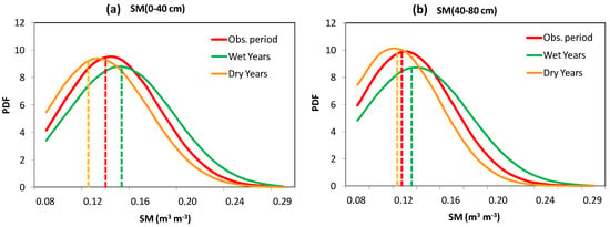
Figure 8.
Fitted normal probability distribution function of the SM in dry and wet years at (a) 0–40 cm and (b) 40–80 cm in the growing season from 2007 to 2012 (excluding 2008) over the transitional climate zone in China. (The dashed line represents the mean values for the different study periods).
4. Discussion
The relationship between the SM and EF is important for research on land–atmosphere coupling. It reflects strong land–atmosphere coupling in the climate transition zones, representing the distributions of water and energy when land surfaces interact with the atmosphere. The results of this study show that synergistic variations in the SM and EF had significant impacts on the regional weather and climate, and this has been confirmed by numerous past studies [7,33,34,35].
We investigated the relationships of land–atmosphere coupling between the SM and EF, GPP and EF, LAI and EF, and NDVI and EF in the climate transition zone of China. The results showed that the latter three relations (GPP−EF, LAI−EF, and NDVI−EF) did not exhibit strong coupling compared with their values in other regions of the world. This can be attributed to the relatively low annual precipitation in the Chinese climate transition zone and the dominance of desert grasslands as the primary type of vegetation that led to less vigorous transpiration. Moreover, the weak vegetation transpiration led to the lack of vigorous vegetation growth and the low values of GPP, LAI, and NDVI. Furthermore (Figure 9), the dry soil and strong incident radiation resulted in the surface precipitation being returned to the atmosphere through the evaporation process in the climate transition zones. Only a small amount of precipitation was absorbed by vegetation, which was not enough to meet the needs of sufficient vegetation growth [9].
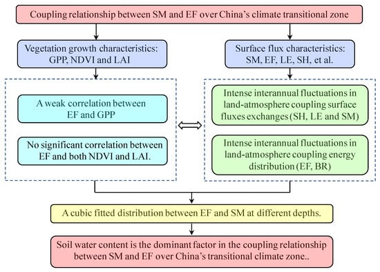
Figure 9.
A flowchart for analysis of the coupling relationship between SM and EF over China’s transitional climate zone.
Overall, the relationship between the EF and SM, as recorded at the SACOL station, exhibited strong coupling that was characterized by non−linear and non−monotonic variations. This result is evident not only from the third−order equations of polynomial fitting of the two variables but also from the segmented relationship of fitting between the EF and the SMP. The turning point in the relationship between the EF and SMP occurred within the SM range of 0.08–0.11 m3 m−3 and was relatively close to the wilting coefficient of soil.
The SM–EF relationship recorded at the SACOL station exhibited a stronger coupling−based correlation than in regions with a humid climate and did not show decoupling when the SM approached or reached saturation, as reported by Williams et al. in 2015 [9]. This was because the soil moisture values in the transitional climate zone are relatively small and cannot reach a sufficiently moist state (>0.3 m3 m−3). Additionally, this characteristic of soil moisture can influence the land–atmosphere coupling relationship [32]. This indirectly indicates the characteristics of a low SM, high ecological vulnerability, and weak resilience against droughts in the area of the SACOL station, which is dominated by desert grasslands.
The coupling relationship between the SM and EF is a crucial parameterization in land surface models [7]. In the transitional climate zone, this strong coupling relationship can offer more options for simulating land–atmosphere exchange processes. Moreover, this constraint relationship between the soil moisture and evaporative fraction, as reflected by SM−EF coupling, is utilized to analyze and assess the drought characteristics of a region [35]. The coupling relationship between the SM and EF is a crucial parameterization in land surface models [7]. This strong coupling relationship can provide more options for simulating land–atmosphere exchange processes in the transitional climate zone. Furthermore, the constraint relationship between soil water moisture and surface fluxes reflected by SM−EF coupling was also used to analyze and assess the drought characteristics in a region [35]. Therefore, in order to more comprehensively illustrate the characteristics of land–atmosphere coupling research in the transitional climate zone, further research is needed on such types of land cover as farmlands and grasslands, which are also part of the climate transition zone.
5. Conclusions
The coupling relationship between SM and EF in the climate transition zone is an important aspect of research on land–atmosphere coupling because it directly reflects the exchange of energy and moisture between the land and the atmosphere. In this study, we applied observation data on fluxes obtained from the SACOL station in the climate transition zone of China to analyze the coupling relationship between SM and EF during the season of vegetation growth. We also explored the relationships between the GPP and EF, LAI and EF, and NDVI and EF that reflect the coupling between vegetation and the atmosphere.
The results indicated that the indices representing the characteristics of vegetation growth, namely GPP, LAI, and NDVI, did not exhibit strong coupling relationships with the EF in the transition zone of China in the summer monsoon. This contrasts significantly with findings on the southern Great Plains of North America. Furthermore, both the components of surface energy and SM exhibited significant interannual variations. The components of surface energy showed the most pronounced interannual differences in July and August. Except for a few extremely wet years, the SM exhibited the greatest interannual differences in August of each year in the study period. An analysis of the coupling relationship between SM and EF revealed that both exhibited strong third−order polynomial correlations, with R-squared values ranging from 0.44 to 0.51 in both the shallower layer (0–40 cm) and the deeper layer of soil (40–80 cm). Further analysis showed that when the SMP reached 35%, there was a significant transition in the linear relationship between the SMP and EF that was consistent between the shallower (0–40 cm) and deeper layers (40–80 cm) of soil.
The SM in the shallower layer (0–40 cm) was higher than in the deeper layer (40–80 cm). Moreover, soils in the climate transition zone of China were characterized by high rates of infiltration of water. The responses of the deep SM to dry and wet years were more significant than those of the SM of the shallow layer. The findings of this study are expected to provide a valuable reference for optimizing the relationships of land–atmosphere coupling in land surface models of the zones of climate transition.
Author Contributions
Conceptualization, Q.Z.; methodology, L.Z. and Q.Z.; software, S.S.; validation, J.W. and Y.H.; formal analysis, L.Z.; investigation, F.Z., S.W. and H.H.; resources, H.L.; writing—original draft preparation, L.Z.; writing—review and editing, S.S.; visualization, J.Z. All authors have read and agreed to the published version of the manuscript.
Funding
This research was funded by the National Natural Science Foundation of China (grant Nos. 42230611, 41875020, and 42005097), the Meteorological Capacity Enhancement Joint Research Special Key Projects (23NLTSZ008), and the Natural Science Foundation of Gansu Province (grant No. 22JR5RA748).
Data Availability Statement
The NDVI data are available at https://doi.org/10.5067/MODIS/MOD09GA.006, accessed on 6 October 2023; and the LAI data are available at https://lpdaac.usgs.gov/products/mod15a2hv061/, accessed on 6 October 2023.
Acknowledgments
The authors thank SACOL and NASA for the data support.
Conflicts of Interest
The authors declare no conflict of interest.
References
- Trenberth, K.E.; Fasullo, J.T.; Kiehl, J. Earth’s global energy budget. Bull. Am. Meteorol. Soc. 2009, 90, 311–323. [Google Scholar] [CrossRef]
- Oki, T.; Kanae, S. Global hydrological cycles and world water resources. Science 2006, 313, 1068–1072. [Google Scholar] [CrossRef]
- Budyko, M.I. Теплoвoй Баланс Земнoй Пoверхнoсти (Heat Balance of the Earth’s Surface); Gidrometeoizdat: Leningrad, Russia, 1956; p. 255. [Google Scholar]
- Koster, R.D.; Dirmeyer, P.A.; Guo, Z.; Bonan, G.; Chan, E.; Cox, P.; Gordon, C.T.; Kanae, S.; Kowalczyk, E.; Lawrence, D.; et al. Regions of strong coupling between soil moisture and precipitation. Science 2004, 305, 1138–1140. [Google Scholar] [CrossRef]
- Seneviratne, S.I.; Lüthi, D.; Litschi, M.; Schär, C. Land–atmosphere coupling and climate change in Europe. Nature 2006, 443, 205–209. [Google Scholar] [CrossRef]
- Teuling, A.J.; Hirschi, M.; Ohmura, A.; Wild, M.; Reichstein, M.; Ciais, P.; Buchmann, N.; Ammann, C.; Montagnani, L.; Richardson, A.D.; et al. A regional perspective on trends in continental evaporation. Geophys. Res. Lett. 2009, 36, L02404. [Google Scholar] [CrossRef]
- Seneviratne, S.I.; Corti, T.; Davin, E.L.; Hirschi, M.; Jaeger, E.B.; Lehner, I.; Orlowsky, B.; Teuling, A.J. Investigating soil moisture–climate interactions in a changing climate: A review. Earth−Sci. Rev. 2010, 99, 125–161. [Google Scholar] [CrossRef]
- Zhang, Q.; Yang, Z.; Hao, X.; Yue, P. Conversion features of evapotranspiration responding to climate warming in transitional climate regions in Northern China. Clim. Dyn. 2019, 52, 891–3903. [Google Scholar] [CrossRef]
- Williams, I.N.; Torn, M.S. Vegetation controls on surface heat flux partitioning, and land-atmosphere coupling. Geophys. Res. Lett. 2015, 42, 9416–9424. [Google Scholar] [CrossRef]
- Zhao, F.; Lei, J.; Wang, R.; Zhang, Q.; Qi, Y.; Zhang, K.; Guo, Q.; Wang, H. Environmental determination of spring wheat yield in a climatic transition zone under global warming. Int. J. Biometeorol. 2022, 66, 481–491. [Google Scholar] [CrossRef]
- Zhang, Q.; Wang, W.; Wang, S.; Zhang, L. Increasing trend of pan evaporation over the semiarid loess plateau under a warming climate. J. Appl. Meteorol. Climatol. 2016, 55, 2007–2020. [Google Scholar] [CrossRef]
- Qiao, L.; Zhang, Q.; Yue, P.; Jin, H. Analysis of changes in the structure of atmospheric boundary layer from non-monsoon zone to monsoon zone. Chin. J. Atmos. Sci. 2019, 43, 251–265. (In Chinese) [Google Scholar] [CrossRef]
- Zhang, L.; Zhang, Q.; Zhang, H.; Yue, P.; Li, H.; Wang, J.; Zhao, F.; Wang, Y.; Wang, J. Environmental factors driving evapotranspiration over a grassland in a transitional climate zone in China. Meteorol. Appl. 2022, 29, e2066. [Google Scholar] [CrossRef]
- Wang, K.; Dickinson, R.E. A review of global terrestrial evapotranspiration: Observation, modeling, climatology, and climatic variability. Rev. Geophys. 2012, 50, RG2005. [Google Scholar] [CrossRef]
- Trenberth, K.E.; Fasullo, J.T. North American water and energy cycles. Geophys. Res. Lett. 2013, 40, 365–369. [Google Scholar] [CrossRef]
- Ford, T.W.; Rapp, A.D.; Quiring, S.M.; Blake, J. Soil moisture-precipitation coupling: Observations from the Oklahoma Mesonet and underlying physical mechanisms. Hydrol. Earth Syst. Sci. 2015, 12, 3617–3631. [Google Scholar] [CrossRef]
- Dirmeyer, P.A.; Zeng, F.J.; Ducharne, A.; Morrill, J.C.; Koster, R.D. The sensitivity of surface fluxes to soil water content in three land surface schemes. J. Hydrometeorol. 2000, 1, 121–134. [Google Scholar] [CrossRef]
- Zhang, H.; Pak, B.; Wang, Y.; Zhou, X.; Zhang, Y.; Zhang, L. Evaluating surface water cycle simulated by the Australian community land surface model (CABLE) across different spatial and temporal domains. J. Hydrol. Meteorol. 2013, 14, 1119–1138. [Google Scholar] [CrossRef]
- Schwingshackl, C.; Hirschi, M.; Seneviratne, S.I. Quantifying Spatiotemporal Variations of Soil Moisture Control on Surface Energy balance and Near-Surface Air temperature. J. Clim. 2017, 30, 7105–7124. [Google Scholar] [CrossRef]
- Basara, J.B.; Crawford, K.C. Linear relationships between root-zone soil moisture and atmospheric processes in the planetary boundary layer. J. Geophys. Res. Atmos. 2002, 107, ACL-10. [Google Scholar] [CrossRef]
- Chen, X.; Su, Z.; Ma, Y.; Sunt, F. Analysis of land-atmosphere interactions over the north region of MT. Qomolangma (Mt. Everest). Arct. Antarct. Alp. Res. 2012, 44, 412–422. [Google Scholar] [CrossRef][Green Version]
- Bi, J.; Huang, J.; Fu, Q.; Wang, X.; Shi, J.; Zhang, W.; Huang, Z.; Zhang, B. Toward characterization of the aerosol optical properties over loess plateau of Northwestern China. J. Quant. Spectrosc. Radiat. Transf. 2011, 112, 346–360. [Google Scholar] [CrossRef]
- Liu, Y.; Huang, J.; Shi, G.; Takamura, T.; Khatri, P.; Bi, J.; Shi, J.; Wang, T.; Wang, X.; Zhang, B. Aerosol optical properties and radiative effect determined from sky-radiometer over Loess Plateau of Northwest China. Atmos. Chem. Phys. 2011, 11, 11455–11463. [Google Scholar] [CrossRef]
- Zuo, J.; Huang, J.; Wang, J.; Zhang, W.; Bi, J.; Wang, G.; Li, W.; Fu, P. Surface turbulent flux measurements over the loess plateau for a semi-arid climate change study. Adv. Atmos. Sci. 2009, 26, 679–691. [Google Scholar] [CrossRef]
- Huang, J.; Zhang, W.; Zuo, J.; Bi, J.; Shi, J.; Wang, X.; Chang, Z.; Huang, Z.; Yang, S.; Zhang, B.; et al. An overview of the semi-arid climate and environment research observatory over the loess plateau. Adv. Atmos. Sci. 2008, 25, 906–921. [Google Scholar] [CrossRef]
- Falge, E.; Tenshunen, J.; Baldocchi, D.; Aubinet, M.; Bakwin, P.; Berbigier, P.; Bernhofer, C.; Bonnefond, J.; Burba, G.; Clement, R.; et al. Phase and amplitude of ecosystem carbon release and uptake potentials as derived from FLUXNET measurements. Agric. For. Meteorol. 2002, 113, 75–95. [Google Scholar] [CrossRef]
- Li, H.; Zhang, Q.; Yue, P.; Zhang, L.; Niu, X.; Zhang, H.; Xing, K.; Jing, Y.; Shang, G. Temporal duration of the East Asian summer monsoon substantially affects surface energy exchange over the summer monsoon transition zone of China. J. Clim. 2021, 34, 4643–4660. [Google Scholar] [CrossRef]
- Vermote, E.F.; El Saleous, N.Z.; Justice, C.O.; Kaufman, Y.J.; Privette, J.L.; Remer, L.; Roger, J.C.; Tanre, D. Atmospheric correction of visible to middle-infrared EOS-MODIS data over land surfaces: Background, operational algorithm and validation. J. Geophys. Res. Atmos. 1997, 102, 17131–17141. [Google Scholar] [CrossRef]
- Allen, R.G.; Pereira, L.S.; Raes, D.; Smith, M. Crop Evapotranspiration—Guidelines for Computing Crop Water Requirements—FAO Irrigation and Drainage Paper 56; FAO: Rome, Italy, 1998; Volume 300, p. D05109. [Google Scholar]
- Li, Y.; Zhang, L.; Zhang, H.; Pu, X. Drought Monitoring Based on CABLE Land Surface Model and Its Effect Examination of Typical Drought Events. Plateau Meteorol. 2015, 34, 1005–1018. (In Chinese) [Google Scholar] [CrossRef]
- Zhang, L.; Zhang, H.; Li, Y. Surface energy, water and carbon cycle in China simulated by the Australian community land surface model (CABLE). Theor. Appl. Climatol. 2009, 96, 375–394. [Google Scholar] [CrossRef]
- Bagley, J.E.; Kueppers, L.M.; Billesbach, D.P.; Williams, I.N.; Biraud, S.C.; Torn, M.S. The influence of land cover on surface energy partitioning and evaporative fraction regimes in the U.S. southern Great Plains. J. Geophys. Res. Atmos. 2017, 122, 5793–5807. [Google Scholar] [CrossRef]
- Qiao, L.; Zuo, Z.; Zhang, R.; Piao, S.; Xiao, D.; Zhang, K. Soil moisture-atmosphere coupling accelerates global warming. Nat. Commun. 2023, 14, 4908. [Google Scholar] [CrossRef] [PubMed]
- Qiao, L.; Zuo, Z.; Xiao, D. Evaluation of soil moisture in CMIP6 simulations. J. Clim. 2021, 35, 779–800. [Google Scholar] [CrossRef]
- Dirmeyer, P.; Balsamo, G.; Blyth, E.; Morrison, R.; Cooper, H. Land-Atmosphere Interactions Exacerbated the Drought and Heatwave Over Northern Europe During Summer 2018. AGU Adv. 2021, 2, e2020AV000283. [Google Scholar] [CrossRef]
Disclaimer/Publisher’s Note: The statements, opinions and data contained in all publications are solely those of the individual author(s) and contributor(s) and not of MDPI and/or the editor(s). MDPI and/or the editor(s) disclaim responsibility for any injury to people or property resulting from any ideas, methods, instructions or products referred to in the content. |
© 2023 by the authors. Licensee MDPI, Basel, Switzerland. This article is an open access article distributed under the terms and conditions of the Creative Commons Attribution (CC BY) license (https://creativecommons.org/licenses/by/4.0/).