Abstract
Floods are the most common and costliest natural disaster in Australia. Australian flood risk assessments (FRAs) are mostly conducted on relatively small scales using modelling outputs. The aim of this study was to develop a novel approach of index-based analysis using a multi-criteria decision-making (MCDM) method for FRA on a large spatial domain. The selected case study area was the Hawkesbury-Nepean Catchment (HNC) in New South Wales, which is historically one of the most flood-prone regions of Australia. The HNC’s high flood risk was made distinctly clear during recent significant flood events in 2021 and 2022. Using a MCDM method, an overall Flood Risk Index (FRI) for the HNC was calculated based on flood hazard, flood exposure, and flood vulnerability indices. Inputs for the indices were selected to ensure that they are scalable and replicable, allowing them to be applied elsewhere for future flood management plans. The results of this study demonstrate that the HNC displays high flood risk, especially on its urbanised floodplain. For the examined March 2021 flood event, the HNC was found to have over 73% (or over 15,900 km2) of its area at ‘Severe’ or ‘Extreme’ flood risk. Validating the developed FRI for correspondence to actual flooding observations during the March 2021 flood event using the Receiver Operating Characteristic (ROC) statistical test, a value of 0.803 was obtained (i.e., very good). The developed proof-of-concept methodology for flood risk assessment on a large spatial scale has the potential to be used as a framework for further index-based FRA approaches.
1. Introduction
1.1. Floods as a Natural Hazard
Floods are among the most hazardous and destructive natural disasters that affect global, regional, and local communities [1,2,3]. The Australian Bureau of Meteorology (BoM) describes a flood as “an overflow of water beyond the normal limits of a watercourse” [4] and is experienced in three major forms—fluvial (the overflow of a water body), pluvial (a result of extreme rainfall, also known as flash-flooding), and coastal inundation (caused by storm surge) [5]. Recent Australian flood events of 2021–2022 have been particularly destructive [6]. The year 2022 alone has seen, notably along the east coast of Australia in southern Queensland (QLD) and New South Wales (NSW), flood events repeatedly devastate communities. As the devastation of these flood events is analysed in their aftermath, crucial questions are being raised in Australia’s flood-prone regions regarding flood assessment and management. It is evident that research into how these frequently flooded regions experience flood risk is required to inform future flood management strategy.
Australia’s highly variable hydroclimate has historically subjected widespread regions to extreme rainfall events that lead to flooding [7]. In many traditional Australian water-based ecosystems, flood events were once a routine occurrence which is typically beneficial to the ecosystem. Such benefits include the distribution of sediments and nutrients across vegetated areas, which greatly assists agriculture, for example [8,9]. It is only after human communities begin to urbanise in these areas, with their infrastructure becoming more exposed, that destructive damages from flood events are experienced. This has become highly problematic in post-colonisation Australia, which commonly features settlements on floodplains [10]. The ensuing damages on a recurring basis in these settled communities have led floods to become Australia’s most expensive natural disaster [11]. More recently, the Insurance Council of Australia has estimated that flood events in 2022—as of May—are responsible for nearly AUD 3.3 billion in insured losses [12]. Deloitte (2021) have estimated that by 2060, flood events, as well as other natural disasters, will lead to a combined annual economic cost for the country of approximately AUD 73 billion [13]. Therefore, the preservation, restoration, mitigation, and resilience-building of flood-prone communities are of crucial importance.
Extreme rainfall events in Australia, especially in areas of NSW, have become increasingly concerning, with research suggesting that they are growing in intensity [14,15]. Multiple factors can be attributed to the intensification of pluvial floods, including important climate drivers such as the Indian Ocean Dipole, the Southern Annular Mode, the Madden–Julian Oscillation, and importantly the El Niño Southern Oscillation (ENSO) [16]. The negative phase of ENSO in particular, La Niña, is typically associated with elevated rainfall totals across eastern regions of Australia [17]. Coupled with anthropogenic climate change, which can contribute approximately 7% more moisture to the atmosphere per degree of warming, La Niña events have been found to be at risk of intensifying [18,19]. The three-year period of 2020–2022 saw three consecutive La Niña events, with corresponding flood events devastating areas of eastern Australia. This underscores the need for a more proactive approach to flood risk assessment.
1.2. Flood Risk Assessment
1.2.1. Risk Assessment
Risk is typically characterised as the probability of a loss and can be calculated as the product of hazard, exposure, and vulnerability elements (Equation (1)) as per Crichton’s Natural Hazard Risk Triangle [20,21]. This representation describes the complex interplay that exists between a given hazard and the corresponding area the hazard impacts, which modulates the extent of loss for a given event.
Risk = Hazard × Exposure × Vulnerability
The quantitative assessment of natural hazards risk is an important method of risk reduction and, in the case of flooding, this is no different. Being a highly trusted and influential body, the Intergovernmental Panel on Climate Change’s (IPCC) definitions provide strong context and guidance to this research, with some important terms being adapted for this study’s scope (see Section 2). In the context of climate change impacts, risks result from dynamic interactions between climate-related hazards with the exposure and vulnerability of the affected human or ecological system to the hazards [22]. In the context of climate change responses, risks result from the potential for such responses not achieving the intended objective(s), or from potential trade-offs with, or negative side-effects on, other societal objectives, such as the Sustainable Development Goals [22].
Exploring the concept of flood risk, the IPCC states that “the risk from flooding to human and ecological systems is caused by the flood hazard (the frequency and/or magnitude of flood events), the exposure of the system affected (e.g., topography, or infrastructure in the area potentially affected by flooding) and the vulnerability of the system (e.g., design and maintenance of infrastructure, existence of early warning systems). Statements about changes in the frequency and/or magnitude of flood events on their own should not be characterised as changes in flood risk, since this covers only the climate-related hazard part. Whether and how much the actual risk, i.e., adverse consequences for human and ecological systems will increase in future (or have changed in the past), will depend also on changes in the exposure and vulnerability of such systems. For example, the damage from flooding could be reduced, even if the frequency of flooding increases, if measures are taken that reduce the exposure and/or vulnerability of affected systems (noting river management in many parts of the world has reduced flood risk)” [22].
Thus, this research defines flood risk as “the potential for adverse consequences for human or ecological systems, recognising the diversity of values and objectives associated with such systems” [22]. Flood Risk Assessments (FRAs) are quantitative evaluations of a region’s risk of flooding using spatial-based inputs such as modelling and remote sensing data, as well as indicator methods [23]. Ali et al. (2016) [24] also describe “essential” tools such as Geographical Information Systems (GIS) software, which is frequently used to compile and evaluate the data in an FRA as well as to produce flood risk indices and maps. Proactive FRAs comprise a vital component of the concept of flood risk management and are a critical resource required to reduce both flood risk and flood losses in vulnerable communities. The ultimate role of an FRA is to highlight the most at-risk areas for flooding, which allows relevant decision makers to allocate resources and initiate mitigatory measures more effectively. As defined by Tiepolo et al. (2021) [25], FRAs typically comprise the following four steps: (i) Context definition; (ii) Risk identification; (iii) Risk analysis; and (iv) Risk evaluation.
1.2.2. Flood Risk Assessment Methods
FRAs are widely conducted using modelling outputs and multi-criteria decision-making (MCDM) methods (e.g., indices). The former is a common approach to FRAs on relatively small scales, and typically produces any of the following: flood hazard/depth/extent models (hydraulic and hydrologic flood models), flood vulnerability/hazard curves, and flood loss models, (e.g., [26,27,28], respectively). These assessments provide highly accurate flood behaviour data at high resolutions; however, this comes with the drawback of being resource intensive [29]. Additionally, this approach generally requires river and basin data, which limits these studies to smaller study areas with appropriate data availability [30].
Conversely, index-based MCDM methods use spatial data inputs with relatively lower resolution (e.g., from remote sensing) to assess flood risk. Completing this with a consideration of each of the risk elements creates a holistic FRA [31]. To do this, sub-indicators of each of the risk elements are standardised and then combined, typically using a form of MCDM such as the Analytical Hierarchy Process, Random Forest Technique, and Fuzzy Logic, (e.g., [32,33,34], respectively). In some instances, flood modelling data is used to provide data for indicator-based assessments, therefore crossover is seen between these two categories of assessment (e.g., [35]). However, whenever modelling data is not used, these MCDM FRAs are considered to be proxy assessments, as they are effectively carried out from afar and do not require any field measurements, for example. These index methods are frequently used to assess the risk of a wide variety of natural hazards, and are commonplace among the international scientific community.
1.2.3. Flood Risk Assessment in Australia
Australian FRAs primarily follow the Australian Institute for Disaster Resilience (AIDR) Flood Hazard Guidelines [27], which outlines best-practice FRA methods using modelling-based approaches. Despite this well-established practice, [36] found significant nationwide variability when it came to the level of flood planning in each Australian Local Government Area (LGA), of which FRAs are a key component. Local councils are given the responsibility of conducting local FRAs, and typically outsource to consulting companies. Consequently, this has created a system of individualistic FRAs on river basin or LGA scales; these studies are often limited in their public data availability. Additionally, FRAs using modelling approaches are flood hazard-centric in their tendency to focus on the flood behaviour characteristics they are modelling, and less so on the other traditional risk components of flood exposure and vulnerability. In a sense, this can lead to a subconscious conflation of the concept of hazard with risk, leading to hazard-based FRAs. This nature of the current Australian FRA landscape exposes two relevant research gaps, as described below.
Firstly, the prominence of modelling-based methods to conduct FRAs in Australia highlights a glaring absence of FRAs using alternative indicator-based methods, as was noted by [37]. The broader popularity and versatility of MCDM methods in natural hazard risk assessment suggests that their absence from Australian FRAs may be a perspective that is missing. Only [34,38] specifically assessed inland flood risk using indicator-based MCDM methods in Australia. As thus, the established nature of indices as a risk assessment method contrasts their sparse usage in an Australian flood context.
Secondly, the predominant modelling-based method is restricted to smaller study areas, both due to the resource-intensive nature of flood modelling data as well as the responsibility being given to local councils to assess their LGA. Yet, the NSW Government’s recent Flood Inquiry [39] highlights the need for larger-scale catchment-wide level knowledge, acknowledging that individual councils are under-resourced. The Inquiry further notes that state governments may be better positioned in managing and mapping catchment-scale flood risk. A greater focus upon catchment-wide flood risk management would prove valuable for decision-making on a local scale because of the importance of river catchment context to localised flood risk characteristics, NSW’s Hawkesbury-Nepean Catchment (HNC) being a prominent example of this. This notion of the need for large-scale FRAs is already supported by studies such as [40], which call for the need for an “evolutionary leap” in this form of assessment.
Ultimately, the use of indicator-based methods in flood risk management is a largely underrepresented perspective that provides a more detailed quantification of flood exposure and vulnerability risk elements. As such, it is clear that Australian communities stand to benefit from expanding this method, given the potential to draw new insights. This aligns with the explicit urging of the NSW Government Floods Inquiry [39] to develop community awareness of local flood risk and to invest in proactive disaster management across all levels of society. Assessments using a more well-rounded indicator-based approach stand as a method to build a holistic understanding of flood risk, being one that quantifies all risk elements. They also give equal focus to exposure and vulnerability in addition to hazard [31]. Linking assessments of different spatial scales to comprise a holistic understanding and assessment of flood risk has been identified as a “challenging task” [41], with this study looking to fit as an intermediary scale between local and national/global assessments. Thus, this research scoped a scalable and potentially replicable indicator-based methodology for assessing flood risk over larger spatial scales in inland Australia.
2. Data and Methodology
2.1. Study Area
The study area of this research was the HNC, which lies to the west of Sydney in NSW, Australia. It spans over 21,700 km2, contains twenty-six LGAs (Figure 1), and is NSW’s longest coastal catchment, stretching from Goulburn, through the Blue Mountains City Council, to the latitude of Newcastle. Figure 2 illustrates the topography of this region, as well as the layout of the rivers in the study area.
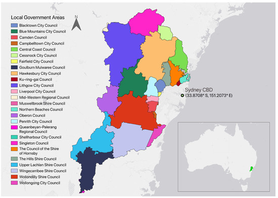
Figure 1.
Australia’s Hawkesbury-Nepean Catchment, visualised through its twenty-six Local Government Areas, as of 2022. Map generated using QGIS 3.24 software.
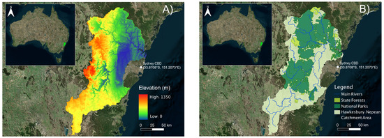
Figure 2.
Topographical and river outline maps of the Hawkesbury-Nepean Catchment region. (A) illustrates the topography, and (B) depicts the conservation areas and river system. Maps generated using ArcMap10.7 software.
There were several reasons for selecting the HNC as the study area for this research. Firstly, this region is widely considered to have the highest flood risk in NSW, if not potentially in all of Australia [42]. This is in part due to the fact that a well-known ‘bathtub effect’ is observed in the heart of the catchment in the Hawkesbury River [42]. The 2019 Hawkesbury-Nepean Valley flood study [43] documents the 18 ‘major’ floods (>12.5 m) that have occurred in the catchment since records began in 1790 to 2019, with a plethora of ‘moderate’ floods (>8 m) also occurring in this period. This alone highlights the severe propensity for flooding in this catchment area. This occurs because there are four major tributaries that feed into the Hawkesbury River, illustrated in Figure 2B, those being the Warragamba, Nepean, Grose, and South Creek tributaries, in addition to other smaller contributing waterways. Crucially, instead of widening closer to the sea, the Hawkesbury River features several tight ‘choke points’ which can quickly cause inundation of the flat floodplain when heavy rainfall events occur and overwhelm the river system (the bathtub effect). Figure 2A highlights the low-lying and flat nature of this central floodplain area, as well as the several surrounding higher-elevated areas that drain into it. Thus, this region is particularly susceptible to flood events in the wake of extreme rainfall events. This, in combination with the highly developed nature of the floodplain area, especially with some parts being of lower average socio-economic status, combines to create a particularly high flood risk catchment. This flood risk is set to increase in the future, with projections outlining a doubling in this catchment’s risk by 2041 due to anthropogenic climate change impacts [39].
Secondly, a catchment with an established propensity for flooding was selected given the better likelihood for relevant data availability for this proof-of-concept work in comparison to a less characterised basin. This is particularly important in relation to the validation aspect of this research, of which the HNC had more available flood observation data to use for validating the Flood Risk Index (FRI) in comparison to other catchments.
Section 2.2 outline the methodology used for the FRA for this study. The novelty of this methodology lies in datasets, including satellite remote sensing data, which were utilised to measure specific indicators, and which are integral to the simplicity and scalability of the study. The overall simplicity ensures that the method has the potential to be replicated over larger spatial scales than are typically studied.
2.2. Flood Risk Assessment Methodology
2.2.1. Scope
The FRA aspect of this research utilised the March 2021 significant flood event that occurred in this area as a case study event [43]. Spatial data used for calculating the FRI, namely the Maximum 3-Day Precipitation (M3DP) and Soil Moisture (SM) indicators, were acquired for this time period. This allowed for an assessment of this catchment area during a high rainfall event that was known to have regional impacts, and thus test our system during a period when high risk values may be expected from this index. The flood event occurred between the 17th and the 26th of March, whereby heavy rainfall over several days in the HNC resulted in the major Warragamba Dam spilling over 450 gigalitres in the downstream floodplain area (as context, this is close to the volume of NSW’s Sydney Harbour, being 500 gigalitres). This led to severe flooding in large parts of the floodplain area [43]. An intense East Coast low pressure system driven by the antecedent La Niña conditions was largely responsible for the extreme rainfall observed [43].
Specifically, the scope of this research entails using data from the March 2021 flood event as a temporal case study; time-dependent data (rainfall and soil moisture) came from within this period. This flood event occurred from the 17th to the 26th of March 2021. Large parts of eastern Australia experienced devastating floods, which killed five people and forced eighteen thousand people to evacuate. Heavy rainfall and wet antecedent conditions influenced by the 2020–21 La Niña event were largely attributed to causing this flooding to occur [43]. Persistent heavy rainfall resulted in the Warragamba Dam, the major dam in the HNC, releasing over 450 gigalitres of water per day for several days. The nearby major city of Sydney receives an average of approximately 1200 mm of rainfall, meaning that the catchment-wide 4-day rainfall average of just above 200 mm comprises a considerable amount of a given year’s rain all across the catchment. This resulted in an estimated AUD 65–97 million in insurance claims alone in this catchment [42]. Nearby regions received over 1200 mm of rainfall for the month of March 2021, which constitutes an entire year of annual rainfall in Sydney [42].
2.2.2. Indicators and Data Collection
There were several factors that contributed to the selection of the indicators that comprised each of the hazard, exposure, and vulnerability inputs that are used to calculate the overall FRI. Firstly, relevant prior literature was thoroughly consulted and strongly informed the inputs that were desired to be used. Secondly, characteristics of this study area and the Australian environment were also taken into account. For example, SM was employed as one of the indicators for the hazard index, as it was deemed to be an important representative of antecedent conditions across various hydrological literature. Data availability issues became an additional factor which limited some inputs from being used in this research. Given that a key element of novelty in this proof-of-concept FRA is the simplicity of the indices, risk components were limited to only 3–4 inputs.
Flood Hazard Indicators and Data Collection
This research defined flood hazard as an adaptation of the IPCC’s definition, being: “the potential occurrence of a natural or human-induced physical flood event or trend that may cause loss of life, injury, or other health impacts, as well as damage and loss to property, infrastructure, livelihoods, service provision, ecosystems and environmental resources” [22].
One of three flood hazard indicators was the Maximum 3-Day Precipitation input. This indicator is quantified as the maximum amount of rainfall received in a given 3-day period. Satellite-based rainfall estimates were used to provide data for this indicator. Rain gauge estimates would also be applicable; however, these are limited to the locations of gauge installations and do not always have a homogenous spatial distribution, which means that the use of satellite data makes this indicator more replicable to other study areas. FRAs using index methods frequently use a form of rainfall indicator, as rainfall is logically a key modulator of pluvial and fluvial flooding events. Some earlier studies, such as [44,45] quantify rainfall in their FRAs using annual rainfall; however, in this study, a 3-day period was chosen given how much more important rainfall over a shorter time frame is in a flooding context. This 3-day precipitation concept is observed sparsely in other literature, such as by [46]; however, it has not been applied in an Australian context. Ultimately, this 3-day period was chosen as a compromise to cover both single-day pluvial floods and multi-day fluvial flooding.
It is acknowledged that radar data are considered the most accurate precipitation estimates over large areas. However, in absence of radar data, precipitation estimates from satellite remote sensing provide an alternative to gauge- or radar-based measurements with greater spatial coverage and improving accuracy. Although meteorological services keep rain gauge records usually dating back decades, satellite precipitation data can complement and potentially improve conventional precipitation records, leading to an improved ability to place extreme precipitation events within a climatological context. This leads to better heavy precipitation and drought monitoring, amongst numerous other applications.
For this study, satellite precipitation data were obtained from the World Meteorological Organization’s (WMO) Space-based Weather and Climate Extremes Monitoring (SWCEM) [47]. For the SWCEM, satellite precipitation datasets were provided by the Japan Aerospace Exploration Agency (Global Satellite Mapping of Precipitation, or GSMaP) and the U.S. National Oceanographic and Atmospheric Administration (Climate Prediction Center morphing technique, or CMORPH). The SWCEM datasets for the East Asia and Western Pacific region (50° E–120° W; 40° N–45° S) are available from the WMO SWCEM website (https://public.wmo.int/en/programmes/wmo-space-programme/swcem accessed on 13 January 2023). A comprehensive analysis of the SWCEM satellite precipitation data performed over Australia showed that blended satellite-gauge products had higher correlations and smaller errors than gauge analysis [48,49,50,51,52,53]. Similarly, earlier studies demonstrated the usefulness of satellite precipitation data not only for Australia but also for countries in the Pacific region [54,55], which means that the SWCEM data as well as the developed in this study flood risk assessment methodology could potentially be used in other countries in the Asia-Pacific region.
Evaluating satellite precipitation estimates, earlier studies found that the Global Satellite Mapping of Precipitation (GSMaP) dataset had high performance over Australia [48,49,50,51]. GSMaP uses the Global Precipitation Mission (GPM) constellation and NOAA Climate Prediction Center 4 km infrared product [56,57]. The version used in this study is the Gauge Near-Real-Time (GNRT) version where the Climate Prediction Center daily global dataset of rain gauges is used to calibrate the GSMaP estimates by roughly matching their values across the past 30 days. Based on extensive validation of GSMaP data over Australia conducted in earlier studies [48,49,50,51] and conclusions that is it a high performing dataset, in this study, using GSMaP data, 3-day precipitation estimation periods from the 17th to the 26th of March 2021 (the length of the flood event; see Appendix D for detail) were calculated, and the highest 3-day precipitation total at each specific grid cell (0.1 degrees resolution) was used for the indicator. The resultant input was a gridded dataset of 3-day accumulation values from a combination of date ranges, depending on which was the highest at each point.
The second of three flood hazard indicators used was Distance to River—Elevation-Weighted (DREW). This input quantifies the distance of any point in the study area to the nearest river. This is an important metric in an FRA context because of how strongly the river locations modulate the locations of flooding in fluvial and pluvial scenarios. Particularly in the HNC, the proximity of a given point to the lower-elevated, downstream Hawkesbury River areas corresponds strongly to flooding outputs. This is the motivation for combining a typical Distance to River input (seen commonly in FRAs) (e.g., [58,59]) with an elevation layer, to capture that lower-elevated areas are more likely to flood after an extreme rainfall event, as opposed to weighting all river areas at different elevation levels equally.
This input was created by calculating the distance of each grid point to the nearest river line using an ‘Euclidean Distance’ function. Then, this layer was multiplied with an elevation layer to account for the influence of elevation. The resulting input described the distance of each point to the nearest river, whilst being weighted as more hazardous if the elevation were lower.
Finally, Soil Moisture was the third input used for the flood hazard quantification. SM is considered an important modulator and representative of the antecedent conditions of an environment. SM has been found to have a direct influence on Australian flood timing, particularly in southern Australia [60]. Other recent literature notes the consensus among Australian research that consideration of changes in the antecedent conditions are crucial to predictive flood modelling [61,62,63]. As thus, SM prior to the case study flooding event, being representative of the antecedent conditions, was quantified in this FRA.
The SM data were collected from the BoM’s Australian Water Resources Assessment Landscape model (AWRA-L), which is a daily gridded SM dataset measuring absolute moisture content in the root zone (0–1 m) [64]. SM content is measured as the amount of water in the soil as a volumetric quantity, for example, a SM percentage of 50% would mean that half of the soil’s total water carrying capacity has been filled. To represent the antecedent conditions of this study area, a 7-day SM average was taken prior to the beginning of the flood event (11 March 2021–17 March 2021).
Flood Exposure Indicators and Data Collection
This research utilised the IPCC’s flood exposure definition as “the presence of people; livelihoods; services and resources; infrastructure; or economic, social, or cultural assets in places and settings that could be adversely affected by a flood event” [22]. Three indicators were chosen to capture flood exposure in the HNC for this study: population density, land use type, and critical infrastructure density.
Population density was selected as an indicator for flood exposure because it is commonly used in FRAs to capture population exposure to floods (e.g., [65,66]). Population density is positively correlated with flood exposure in that an increase in population density results in a proportional increase in people directly exposed to flood exposure. This indicator was available at the Statistical Area 2 (SA2) level and was sourced from the Australian Bureau of Statistics (ABS) via a 2021 regional population estimate dataset. It was then rasterised using QGIS 3.24 software, being cut to boundaries applicable to that of the HNC. Importantly, density was calculated in particular as this standardises between differently sized SA2s.
Land use type is an important indicator for a Flood Exposure Index (FEI) because it ranks different land use types based on the extent to which they are flood-exposed, indicating which land use types are associated with the greatest cost (e.g., [65,67]). This indicator can be correlated to flood exposure by assigning values to land types (e.g., [58]), where higher values indicate greater flood exposure. The land use type analysis for this study prioritised the built environment, such as infrastructure and roads (note that it remains different to the critical infrastructure density indicator described below). Capturing these elements is critical to a flood exposure analysis as inland flooding is, as mentioned, prevalent in urban environments, which may present poorer flood-conscious urban planning. For this study, this indicator was sourced as a 50 m vector from the NSW Government’s 2017 Land use v1.2 dataset. It was then rasterised and cut to HNC boundaries. Importantly, this clipped dataset had thirty-one land use types, which was too complex for this study’s scope. Therefore, the dataset was reclassified into a subset of eight: water bodies, nature conservation, forestry, cropping, grazing, horticulture, infrastructure, and other. Such reclassification is common in the literature (e.g., [68,69]). Having done this, a flood exposure value with a respective rating was then assigned to each reclassified land use type, as described in Table A1, Appendix A.
Critical infrastructure (CI) density, which describes the amount of CI over a given land area, is critical to an FRA because it again captures the flood-exposed built environment (e.g., [70,71]). This study assumes eight CIs: roads (including State Emergency Service (SES) evacuation routes), power stations, power substations, electricity transmission lines, hospitals, police stations, SES offices, and broadcast transmission towers. Importantly, these CIs capture important services and utilities such as transport, emergency services, and communication. CI density is positively correlated with flood exposure in that an increased CI density results in greater flood exposure. All CI datasets were downloaded as vectors, rasterised, and cut to HNC boundaries. It should be noted that roads were defined as dual carriageways, principal roads, secondary roads, and SES-recommended evacuation routes. CI density was calculated in particular because SA2s in the HNC vary significantly in size and CI density is a way of standardising between such SA2s.
Flood Vulnerability Indicators and Data Collection
In accordance with the IPCC definition, flood vulnerability was defined as “the propensity or predisposition to be adversely affected. It encompasses a variety of concepts and elements, including sensitivity or susceptibility to harm and lack of capacity to cope and adapt” [22]. In this study, three categories of flood vulnerability were addressed: environmental, social, and economic. The indicators that were chosen to measure these categories were elevation, degree of slope, Index of Relative Socio-economic Disadvantage (IRSD), and Hydrologic Soil Groups (HSG).
The elevation of the area was investigated as a component of the topography of the HNC. The height at which land lies impacts the movement and drainage of water [72,73]. As a physical indicator, elevation shows the highest vulnerability where the lowest-lying areas occur, as water flows from higher- to lower-elevated areas. It was important to investigate this indicator in order to understand the influence of topography on the vulnerability of communities. The elevation at which communities place their residencies and infrastructure could contribute to the overall risk of the area.
Often found coupled with elevation in many datasets, the degree of slope is the percentage of change in elevation over a certain distance [74]. It describes the shape and relief of the land as opposed to the height of the land. Slope is calculated using Equation (2):
Slope = Difference in Height/Horizontal Distance
This indicator was chosen as it complements elevation data and has been frequently used in past international flood vulnerability assessments [75,76,77]. Slope influences the speed at which water travels, meaning that in areas with a higher degree of slope, water will run off more readily. The result can be highly sloping areas receiving less pooling of rainwater and thus a lower flood risk. The runoff from sloping areas can also result in a high vulnerability region if directed into a low-lying, flat area [76,78]. In this scenario, low slope is associated with higher vulnerability.
The Index of Relative Socio-economic Disadvantage (IRSD) is an index designed by the ABS as a component of the Socio-Economic Indexes for Areas (SEIFA) product. It comprises sixteen indicators that describe the relative disadvantage of areas. The IRSD is beneficial as a chosen indicator as it encompasses both social and economic aspects of the HNC. IRSD scores are mapped using quintiles. The lowest scoring 20% of areas are given a quintile number of 1, the second-lowest 20% of areas are given a quintile number of 2 and so on, up to the highest 20% of areas which are given a quintile number of 5. Low IRSD scores indicate that an area has a relatively greater disadvantage in general. For example, areas that have low IRSD scores may have (i) many households with low incomes, and/or (ii) many people with long-term health conditions or disabilities, and/or (iii) many dwellings that are overcrowded. Conversely, areas with a high IRSD score would present a lack of disadvantage, meaning, for example, (i) few households with low incomes, and/or (ii) few people with long-term health conditions or disabilities, and/or (iii) few overcrowded dwellings. Low IRSD scores indicate higher vulnerability to loss during a flood event.
Hydrologic soil groups (HSG) were used as an additional environmental indicator. HSG measures the ability of different soil types to absorb water. Soil properties play an important role in flood water and runoff behaviour [79,80]. HSG infiltration behaviour ranges from group D (very low) to group A (high). Lower infiltration rates mean that water is not readily absorbed into the soil. High infiltration means that water is very readily absorbed into the soil. The variation of infiltration behaviour is dependent on soil type, texture, grain size, and aggregate size. Low infiltration rates and their subsequent high runoff potential result in greater vulnerability. Table 1 contains a description of each HSG and its relationship with runoff.

Table 1.
Hydrologic soil classes with corresponding infiltration behaviours and runoff potential. Information sourced from [81].
Table 2 outlines the Data Collection process for each of the flood risk inputs across the three risk elements.
Table 2.
Flood Risk Index data collection. All data is licensed under the Creative Commons CC BY 4.0 license.
2.2.3. Data Standardisation and Index Creation
The data in the FRI was standardised using Fuzzy Logic methods, a two-step process using the fuzzy membership and fuzzy gamma overlay functions in ArcMap10.7 software, which takes raw inputs and produces standardised (values from 0 to 1) data. Appendix B features a Table A2 that describes how each of the indicators has been standardised in this process, and describes the fuzzy gamma overlay equations. This form of data standardisation and index creation is common in FRAs (e.g., [35,58,82,83]). Fuzzy large and small membership sets are created using a ‘midpoint’ and ‘spread’ value; the midpoint being the middle value that the data is standardised away from (becoming 0.5), and the spread value being how strongly the data is spread away from the midpoint. Once all of the individual data were standardised, these were processed with fuzzy gamma overlay to create each of the risk component indicators. Following this step, the three risk components were then combined using fuzzy gamma overlay function to create the overall FRI. Figure 3 outlines the general methodology for creating indices using a fuzzy methodology. For more detailed information regarding the creation of the risk component sub-indicators, see [84,85,86] for flood hazard, exposure, and vulnerability, respectively.
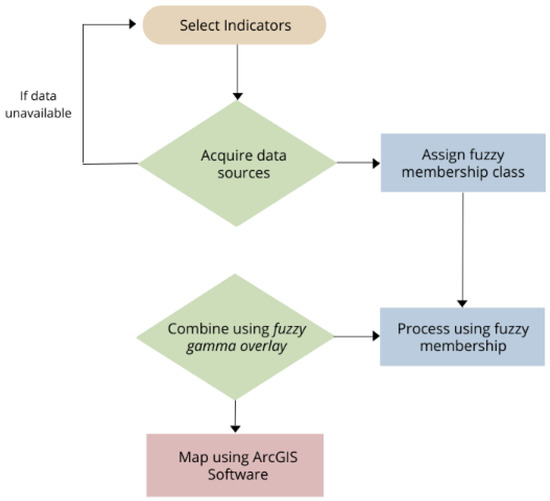
Figure 3.
A methodological flowchart outlining the creation of an index using fuzzy tools.
2.2.4. Index Validation
A newly created index requires validation in order to ensure the results are valid and possess utility for decision makers. Validation of an FRI is a common element of a scientific publication of this form of research, e.g., [58,87]. The methodology for validating an FRA varies across the literature; however, [88] notes that there are three predominant flood risk model validation methods, (i) comparison with observed data, (ii) benchmarking with other models, and (iii) using expert knowledge and expectations. According to this current practice study, (i) is most preferred when observed data is available, followed by (ii) and (iii), in that order. A popular form of comparison with observed data is using the Receiver Operating Characteristic (ROC) statistical test (also known as the Relative Operating Characteristic), as seen in, for example, [33,44,45,89,90]. In the context of a predictive FRA, a better ROC score relates to higher index values aligning to observed flood points [91]. The ROC test calculates the ratio of true positive rates to false positive rates (in this case, high index values that corresponded to flooding observations against high index values that did not flood), and quantifies this test score as the Area Under the Curve (AUC). These true positive and true negative rates are calculated in accordance with Eq. 3 and Eq. 4. The AUC scores on this test range from 0.5 (on par with random guess) to 1 (theoretically perfect alignment), which, according to [92], scales from “0.5–0.6: poor, 0.6–0.7: medium, 0.7–0.8: good, 0.8–0.9: very good, and 0.9–1: excellent”. This was the test used to validate this FRI.
True Positive rate = True Positives/(True Positives + False Negatives)
False Positive rate = False Positives/(True Negative + False Positive)
In this research, the ROC test was calculated using ArcMap10.8 software. This was carried out using the ArcSDM package available online. The flood observation points used for this validation were sourced from [93]. This dataset features flood observation maps from the Wiseman’s Ferry and Western Sydney areas located in the HNC from the March 2021 case study event. Figure 4A illustrates the location of this combined observation area relative to the HNC, and Figure 4B shows the flood observation data itself. These two observation areas combined comprise 2332.61 km2, which is approximately 11% of the catchment area and considered sufficient in size to validate the index (as this size is larger than most FRAs themselves). An arbitrary rectangular area was chosen around these validation areas to encompass a full range of index values from “Very Low” to “Extreme” for the validation study, illustrated in Figure 5. In this figure, one can see that the flood area is relatively small according to Copernicus satellite data, which describe the spread of the flood. Further reasoning for this decision was that the Copernicus dataset highlights the areas that experienced flooding in this event, so it follows that the regions around the Copernicus dataset did not. Thus, this arbitrary area was utilised as a further section of ‘Not flooded’ data in order to encompass this wider range of “Very Low” to “Extreme” data to properly calibrate the validation model.
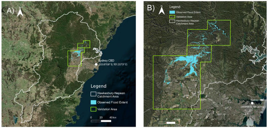
Figure 4.
(A) The location of the observation area relative to the HNC study area. (B) The flood observation data via Copernicus.
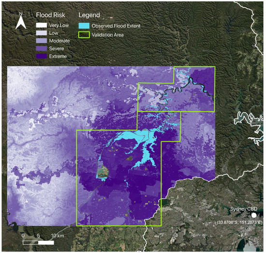
Figure 5.
The location of the FRI data used for validation as well as the flood observation area.
3. Results
3.1. Flood Risk Index
In this study, standard quintile classifications were chosen for the Flood Risk Index along with a severity class according to Table 3.
Table 3.
Breaks assigned to fuzzy values for flood risk indicator maps as well as the overall index map.
Standard quintile classifications are used to simplify the dataset into five basic classes. This is to improve the readability of the data and allows labels to be attributed to these classes (Very Low–Extreme) in the same manner to any similar literature cited. In this sense, these standard classifications are deemed appropriate. Fuzzy Membership and Gamma Overlay are used as standard practice in this field of research, e.g., [58,82]. Essentially, the usage of Fuzzy Membership allows for higher risk index values to have a stronger weighting in the dataset, and lower risk datapoints to contribute less and have lower weighting—this is commonplace in flood risk assessment literature using Fuzzy Logic.
3.1.1. Indicator Maps
Figure 6A–C illustrates the flood risk components: flood hazard, exposure, and vulnerability, respectively. The inputs used to create each of these risk component indices are shown in Figure A1, Figure A2, and Figure A3, (respectively) (Appendix C).
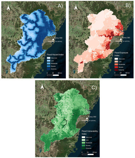
Figure 6.
The three flood risk components: (A) hazard, (B) exposure, and (C) vulnerability. Darker areas indicate greater index values.
3.1.2. Index Map
Figure 7 illustrates the Flood Risk Index for the Hawkesbury-Nepean Catchment. Table 4 illustrates the breakdown of the relative and true size of each flood risk category.
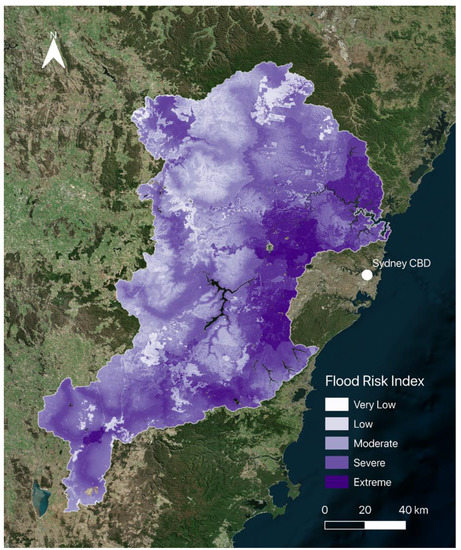
Figure 7.
The Flood Risk Index of the Hawkesbury-Nepean Catchment. Darker areas indicate greater flood risk.
Table 4.
Percentage and total area breakdown of the FRI per each risk class.
The FRI, as expected, comprises some of the major features of each of the flood risk components, particularly those mentioned in Section 3.1.1. Namely, this index visibly features prominent imprints of the river layer in parts, some characteristics of the FEI (the elevated Goulburn area and central Blue Mountains corridor), and general accentuation of the floodplain region, which is particularly characteristic of the Flood Vulnerability Index (FVI). The FRI has additional pockets of isolated extreme flood risk, located in the south of the floodplain in the Upper Nepean State Conservation Area, north-east of the floodplain in Wiseman’s Ferry, and to the north of Lithgow City Council in the HNC’s north-west. As per Table 4, these Extreme areas comprise 24.10% of the study area. Beyond this, the study area demonstrates areas of Very Low–Moderate FRI values, particularly in the central and west of the HNC surrounding the floodplain, approximately accounting for a combined 27.00%. Filling in all other areas are the Severe risk areas, which are the majority of the catchment (49.10%). There is a broader trend, particularly forthcoming in the FEI, of reducing index values away from the coastline and this is similarly discernible in the FRI.
3.2. Index Validation
Figure 8 depicts the result of the ROC validation test, which, according to the aforementioned scale by [92], illustrates a ‘Very Good’ validation result of 0.803 area under the curve.
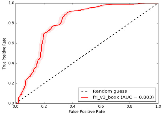
Figure 8.
The Receiver Operating Characteristic test showing the area under the curve as the means of validating the FRI.
4. Discussion
4.1. Flood Risk
Global, regional, and local communities around the world are prone to hydro-meteorological hazards, such as floods, which often turn into disasters threatening livelihoods and causing economic damage to at-risk communities [1,2,3]. In a changing climate, the frequency and severity of hydro-meteorological extreme events, including floods, is increasing [22] and developing novel FRA methodologies which could be easily replicated is an important topic of risk assessment research. To address this topic, a number of regional and national flood risk indexes have been recently developed. For example, the use of the Geomorphic Flood Index (GFI) method for hazard classification has been recognised as a reliable approach. The GFI was proposed by Samela et al. (2017) [94] and Manfreda and Samela (2019) [95] to generate flood extent maps and the methodology is particularly suitable for data-scarce areas. The method is effective for a large study area, in which the flow accumulation values of the whole river basin are needed for the GFI calculation and floodwater depths analysis.
Recently developed multi-criteria decision-making (MCDM) methods are also being used to construct a decision-making process that is more participatory, rational, and efficient. Pathan et al. (2022) [96] used a statistical MCDM approach to generate flood risk maps together with hazard and vulnerability maps in a GIS framework for Navsari city in Gujarat, India, to identify the vulnerable areas that are more susceptible to inundation during floods. Quesada-Román (2022) [97] analysed and classified the 82 Costa Rican municipalities in terms of hazard, exposure, and vulnerability to floods, and then designed an index for flood risk at a local (municipal scale) level. Regional flood risk assessment in mountain catchments in Costa Rica impacted by tropical cyclones was also conducted [98]. The flood risk assessment was based on a high-resolution mapping of infrastructure, population density (as a measure of exposure), and a social development index (to represent vulnerability) and it was shown that regional flood risk assessments can be performed in large-scale catchments if both coarse and detailed inputs are used [98]. Importantly, the results of this study could be useful for the development of flood risk schemes promoting the resilience of local populations. A MCDM method was also used by Ikirri et al. 2022 [99] for the developing flood hazard index and mapping of the flood zones of the Taguenit basin in southern Morocco. The flood risk public perception in flash flood-prone areas of Punjab, Pakistan was examined, contributing to the development of an appropriate management plan for flood risk and communication strategies [100]. A regional study for Europe on future-oriented flood risk management across policy domains on the scale of river sections and catchments has also been conducted, exploring an approach which builds on the understanding of floodplains as coupled human and natural systems [101].
This brief overview demonstrates the breadth and depth of FRA research and application conducted for different regions around the world—Central and Latin Americas, Africa, Asia, and Europe. Further information on modern approaches to the modelling and management of flood risk, with a focus on urban areas, can be found by readers in a comprehensive review by Cea et al. 2022 [102].
In the following sections, we discuss the findings of our case study for the Hawkesbury-Nepean Catchment (HNC), outlining the novelty of the applied MCDM method for Australian FRAs, examining the performance of flood hazard, exposure, and vulnerability indices and overall flood risk index.
4.1.1. Indicators
In this section, the flood risk components (hazard, exposure, and vulnerability) as well as the overall flood risk index (FRI) will be discussed; an analysis of the indicators that comprise them are excluded for brevity.
Note the prominence of the river locations in the Flood Hazard Index (FHI) in Figure 6a. Visually, this input is highly dominant in comparison to the other layers, particularly in the floodplain region where river density is high and tributary convergence is occurring to create the aforementioned bathtub effect. Also noticeable in this index is the signature of the Soil Moisture gridded data in the floodplain region to the west of the Sydney CBD marker. Figure 6b’s FEI highlights a significant concentration of exposure in the floodplain region. This index also features other isolated areas such as Goulburn in the HNC’s south and the central corridor that lies between the major central areas of National Park (see Figure 6c for reference). Similarly, the FVI underscores the extreme flood vulnerability of the floodplain area given its low elevation and widespread lack of slope. This is contrasted with broad regions of low vulnerability in the large areas of National Park directly to the west of the floodplain, where rainfall easily runs off into the floodplain.
Figure 6a’s illustration of the FHI clearly demonstrates the dominance of the Distance to River—Elevation-Weighted (DREW) input, as noted earlier by [84]. One can observe the lines of the rivers strongly modulating the hazard risk values. Given the river lines correspond to a maximum index value of 1 after the standardisation process, these strong results are a logical result as there is no other input to the FHI features values that reach this maximum value. Another consequence of the strength of the DREW input in the FHI is the large block of ‘Extreme’ flood hazard risk situated in the floodplain area of the catchment. This occurred due to high river density and low elevation in this region in addition to the high rainfall and broadly high soil moisture during the case study flood event. Additionally, as aforementioned, the gridded SM data is directly visible in the FHI specifically in the floodplain area. The gridded signature of the SM data is visible, potentially indicating consistency in M3DP and DREW; hydrologically this seems reasonable as soils are likely to experience lagged moisture absorption compared to M3DP and DREW layers, which capture relatively real-time rainfall and river conditions. Ultimately, having the ability to clearly attribute trends to single indicators in this manner is in part a benefit of using only three sub-indicators for each risk element to maintain the novelty of simplicity. This makes analysis of indices such as this far easier than in studies with more inputs, which often require tools such as ‘spider plots’ to assess indicator contribution (e.g., [90]).
The FEI shown in Figure 6b is comparable in this analytic sense. The close relationship between urban growth and flood exposure risk as described by this FRI was noted in earlier research [86]. Importantly, the highly urbanised area in this case study again aligns with the floodplain, the same region which features high index values in each of the three risk component indices—each for separate reasons. In this case, the floodplain zone contains a large majority of the infrastructure and population density of the HNC, resulting in this area being the most flood-exposed according to this index. This is corroborated by the recent NSW Flood Inquiry [39], which details that development in the floodplain is the single largest driver of flood risk in the region. This is also due to the way in which this study was designed; as flood exposure was defined with a focus on human health and livelihoods, it is logical that human infrastructure was placed as the highest priority when it came to quantifying critical infrastructure, leading to this index’s result. Overall, this FEI successfully quantified the extreme flood exposure in the floodplain in a manner that is widely supported by the existing knowledge of this catchment. This includes examples such as the reference by the Insurance Council of Australia that the Hawkesbury-Nepean Valley has the “highest flood exposure in New South Wales, if not Australia’’ [103]. Therefore, the FEI is sufficiently capable to capture flood exposure in studies with replicated methodology.
The FVI shown in Figure 5c demonstrates the vulnerable nature of the floodplain region in particular [85]. This area is denoted by its widespread ‘Extreme’ flood vulnerability, which is largely a result of the low elevation and lack of slope across the district. The result of this index accurately reflects the highly vulnerable nature of this catchment, particularly with respect to the aforementioned hydrological environmental conditions, which have created the bathtub effect. These conditions are well-documented, with studies such as [104] noting the ability of the rivers here to rise much higher than similar catchments in a flood event with a similar frequency. In addition to the characterisation of the physical vulnerability of the study area, the socio-economic vulnerability of the HNC is also quantified through the IRSD input. This indicator highlighted the disadvantage that is observed in the western suburbs of Sydney (especially compared to central Sydney areas), and this only contributes further to the overall vulnerability of the HNC. Furthermore, there appears to be an interplay between these physical and socio-economic vulnerabilities, whereby an area that is prone to and experiences natural hazards (and is evidently physically vulnerable) can attract those experiencing socio-economic disadvantage given the reduced demand, and thus cost, to live in this area. Thus, the HNC is an example of an area with complex vulnerability interplay that is well-captured by this FVI.
4.1.2. Flood Risk Index
The FRI produced uses the three flood risk component sub-indices to comprise an index that highlights areas at risk of flooding, in this case in the HNC. Continuing the trend of each of the incorporated indices, the floodplain area located in the central-eastern quadrant of the study area demonstrated broad regions of ‘Extreme’ flood risk during the March 2021 flood event. Given that each of the risk components produced high index values in this area, it is unsurprising that parts of the floodplain resulted in ‘Extreme’ results. Additionally, smaller isolated regions demonstrated comparatively elevated values of ‘Extreme’ and ‘Severe’ flood risk during this time. Goulburn, in the far south of the HNC, showed ‘Extreme’ FRI values that are most prominently attributable to the ‘Extreme’ flood exposure in addition to elevated flood hazard. Parts of the National Park area to the floodplain’s north were another such outlier of sorts, with multiple tributary rivers and the downstream parts of the Hawkesbury River flowing in this region, in addition to high FEI values. As the Hawkesbury River is the key outflowing waterway to the sea in the HNC—and this National Park area is downstream of the aforementioned ‘choke points’ that heighten flood risk in the floodplain—it is understandable that this area should have elevated flood risk given the sheer amount of water that would flow through here in a flood event. The LGA of Lithgow City Council in the HNC’s north-west was a final example of comparatively elevated flood risk. This area displays ‘Extreme’ flood vulnerability in combination with high river density (thus leading to ‘Extreme’ flood hazard), which together are strong contributors to this final result.
The lingering fingerprint of the river locations in the FRI is similar to the FHI. Visible across the central-western and northern regions of the HNC where lower flood risk is observed, the river lines have been relatively clearly imprinted onto the FRI. In a similar manner to the FHI, this may occur due to consistency across the other indicators, meaning that high values from this indicator are the major point of difference. It is logical that an index focused primarily on flood risk to human health and populations will naturally comprise lower flood exposure and vulnerability index values in areas lacking population and infrastructure. This has ultimately meant that any strong variability across these regions will come from the FHI, of which the DREW indicator displays the strongest variation. Furthermore, there often seems to be one risk component being low in particular that tends to make these areas relatively low risk—this can be understood through the Natural Hazard Risk Triangle, conceptualised in Section 1.2. Based on this framework, a triangle with two long sides and one short side will have a considerably lower area (and thus risk in this case). For example, the north-west region showing lower FRI values may be specifically linked to extremely low FEI values, as there is no population and no infrastructure there. Similarly, the central-western region experiences consistently low FVI values in addition to lower FEI in parts. This may be strongly linked to the high slope and elevation observed in this area, as this is largely the Blue Mountains National Park. It is this broader pattern of lower FEI and FVI towards the western boundary of the HNC that explains this similar trend observed in the FRI. In summary, this research analyses multiple catchment-wide trends that would not have been possible without such a large study area.
4.2. Index Validation
The ROC validation test of the initial FRI produced an AUC score of 0.803, as illustrated in Figure 7. Copernicus data provide aerial coverage and suits this validation exercise best, while data available from just a few locations would not be able to present an accurate representation of the entire study area. Furthermore, the use of Copernicus data ensures consistency and uniformity across the dataset as opposed to a few standalone key locations. This study draws great benefits from the ability to observe a validation study from long lengths of the key rivers. According to the test ranking scale outlined in Section 2.2.4, this is a ‘Very Good’ result [92]. Given the frequency at which this test is used in relevant literature to validate FRAs (e.g., [33,44,45,89,90]), this result is very positive, and highlights the validity of our created index. This validation shows the FRI is a reliable source for decision makers in the HNC, something that was originally a key goal of this work. This retroactive proof-of-concept research can now add to the pool of legitimate research and evidence that exists for this extremely flood-prone catchment. Being the first FRA of this size and nature completed here, it has potentially revealed new data and insights for this catchment.
The FRI presented in this study puts forward a simple, low-cost resource, yet scalable methodology assessment of fluvial and pluvial flood risk. The majority of Australian FRAs currently completed by consulting companies at LGA levels do not possess the above traits, which highlights the novelty of this research. Whilst the current popular methodology may provide more detailed results for smaller study areas, there is potential for this presented methodology to complement what is already used. Therefore, this validated methodology stands as a viable alternative, with the potential to assess large areas more efficiently than is carried out presently. It could be successfully used in addition to the current methods to reveal catchment-wide information and trends, as well as serve as a middle spatial scale to help link national/global and local scale assessments [39]. At the very least, this methodology can be replicated and applied to other at-risk catchments in Australia, if not beyond.
4.3. Future Research Opportunities
Although shown to be valid, this work may ultimately exclude other relevant risk factors given the lesser number of indicators used in comparison to other similar studies (e.g., [34,44,90]). An additional noteworthy point is that data availability strongly limited what indicators were able to be selected for this research. However, there does exist some balance between an overly simplistic FRA and one that is too convoluted and features overlapping risk factors. For example, [85] outlines an instance in [87] which features both ‘River Distance’ and ‘Waterway and River Distance’ as separate flood hazard indicators, both of which may be considered to be overlapping inputs. Thus, there may be additional inputs that could add value to this index, but given the good performance on the validation test, this is not the most pressing issue. A potentially more important problem is the presence of ‘gaps’ that are visible in the FRI.
Upon visual inspection of the FRI, one may notice small data ‘gaps’ present in the index that contain ‘No Data’ and show the base map underneath. This means that somewhere in the index creation process, there was either a ‘0’ or ‘No Data’ value that, when combined with the other indices, was carried through to the final index. These areas mostly comprise water bodies such as the notably large Warragamba Dam to the south-east of the floodplain, indicating that this issue is linked to an input’s quantification of water bodies. Analysing the data that comprised this index, one can note gaps of similar appearance in the FVI, highlighting that this issue must have originated from here, specifically from a combination of the Hydrologic Soil Groups and slope datasets after analysis of [85]. Having gaps such as these present in the dataset is problematic and potentially limiting because it may alter any statistical analysis as the data from these spots are not present in the analysis, for example in the validation study. It may also limit utility to decision makers as there may be data lacking in areas that are important to them. However, these gaps are a common occurrence in this field of research, with one method of addressing this issue being the use of data interpolation.
Future research involving this FRI should primarily surround the expansion of the index to other study areas, as this element of potential replicability was a key aspect of novelty for this research. The capability of this index to assess large-scale regions means that it has the potential to cover large places (such as Australia) with relative ease in comparison to other more resource-intensive methods. As such, it appears that a logical next step for this FRI would be to expand across Australia, based on catchment divisions. Ultimately, the expansion of this index into new study areas would allow for the production of new insights from an FRA perspective, which is relatively unheard of in the Australian landscape.
Additionally, future research involving this FRI should address the aforementioned limitations. For example, the relevant layers in the FVI should be reproduced to remove the ‘gaps’ that exist within this index—chiefly over water bodies. This could require the changing of any ‘0′ or unavailable data areas to real values, which could be carried out by taking an average of all the points surrounding the hole, by applying interpolation methods. Secondly, the Distance to River—Elevation-Weighted (DREW) input could be reiterated to better account for the differences in flow and how this relates to differences in flood hazard. Additionally, the validation study could benefit from iterating on the observation dataset by seeking a dataset that is more representative of the catchment as a whole, which could produce improved findings. Similarly, the FEI could be reiterated to better capture the variability in the amount of people that each sort of critical infrastructure services. For example, this could be carried out by creating a multiplier for each type of infrastructure based on the relative amount that each is used by the community (e.g., number of hospital admissions, number of SES/police callouts, or road usage statistics).
Developing flood risk maps considering the magnitude of precipitation could also be an interesting avenue to further explore risk research approach, e.g., using a 100-year return period [105]. Furthermore, a key feature of this (and all) assessments is the comparative nature of the risk analysis. Whilst it is true that the exact risk percentages will change depending on the event, this data is in some ways relative as it strongly considered the rainfall input, which changes from event to event. An important aspect of this study is simply to note the areas that demonstrate higher risk than others comparatively in the catchment. This reveals important information to decision makers regarding resource allocation and aids the prioritisation of flood risk mitigation in higher-risk areas.
Finally, an evaluation of the performance of the developed FRI with other state-of-the-art methods is recommended for future research. The use of the Geomorphic Flood Index (GFI) method for hazard classification [94,95] has been recognised as a reliable approach and thus could be applicable for comparison with the developed FRI for flood risk assessment over large study areas in Australia.
5. Conclusions
The overall aim of this study was to create and map a scalable and replicable proof-of-concept Flood Risk Index for New South Wales’ Hawkesbury-Nepean Catchment (HNC). The indicators chosen for the FRI were based on flood hazard, exposure, and vulnerability subcomponents. While earlier studies have presented results for flood risk mapping using GIS for relatively small areas, e.g., for the Greater Toronto Area [106] and the Shangyou, China [107], this study, to the best of our knowledge, is the first attempt to develop this novel approach of index-based analysis using satellite remote sensing data, GIS, and a MCDM method for FRA on a large spatial domain (HNC, over 21,700 km2).
The developed FRI suggests that extreme flood risk largely occurs on or near the floodplain of the catchment, that is, in broad areas to the west of Sydney CBD. The HNC was found to have over 73% (or over 15,913 km2) at ‘Severe’ or ‘Extreme’ flood risk during the March 2021 flood event. The positive result of the Receiver Operator Characteristic validation test highlights the validity of the index-based methodology for flood risk assessment.
This study represents a robust proof-of-concept for an inland flood risk index for NSW’s Hawkesbury-Nepean catchment on a novel spatial scale and simplistic method that is novel in the Australian FRA landscape. It is hoped that both the methodology and key findings of this research can be applied elsewhere in Australia, so that relevant stakeholders can assist those communities most affected by potentially more frequent and intense floods. A number of local and regional stakeholders, such as the disaster management offices, City Council planning departments including spatial and urban planners, water management authorities, politicians, NGOs, and representatives of at-risk communities could be involved in and benefit from such FRA. The use of an open source data and the overall simplicity of the developed methodology ensures that it has the potential to be replicated over larger spatial scales, e.g., for a state, territory, or even on the national scale. To assess and map flood risk using the developed methodology, a basic set of skills for stakeholders is needed, e.g., familiarity with ArcGIS. Additionally, as we used the SWCEM satellite data which are provided by the WMO for the East Asia and Western Pacific, we believe this approach could be beneficial for countries in the Asia-Pacific region.
This study presents a contribution to the discussion of flood mitigation and adaptation in Australia and has the potential to be used as a framework for further index-based flood assessment approaches. The logical next steps for the Flood Risk Index surround the expansion to wider areas of Australia and beyond. This is given the focus of creating an index that can easily assess larger areas in a replicable manner. Overall, assessment and mapping of flood risk for at-risk communities (locally, nationally, and regionally) is a valuable contribution to implementing the Sustainable Development Goals, particularly the Sustainable Cities and Communities (goal 11), Climate Action (goal 13), and Life on Land (goal 15).
Author Contributions
Conceptualisation, M.K., I.S., M.Z., A.B.W. and Y.K.; methodology, M.K., I.S. and M.Z.; software, M.K., I.S. and M.Z.; formal analysis, M.K., I.S. and M.Z.; investigation, M.K., I.S. and M.Z.; resources, A.B.W. and Y.K.; data curation, M.K., I.S. and M.Z.; writing—original draft preparation, M.K., I.S. and M.Z.; writing—review and editing, M.K. and Y.K.; visualisation, M.K., I.S. and M.Z.; supervision, A.B.W. and Y.K.; project administration, A.B.W. and Y.K. All authors have read and agreed to the published version of the manuscript.
Funding
This research received no external funding.
Acknowledgments
Authors express sincere gratitude to colleagues from the Climate Risk and Early Warning Systems (CREWS) team at the Australian Bureau of Meteorology and Monash University for their helpful advice and guidance. Two anonymous reviewers and an academic editor provided valuable comments which helped to improve the quality of the manuscript.
Conflicts of Interest
The authors declare no conflict of interest.
Appendix A
Table A1.
Reclassified land use types for the land use type indicator, with respective flood exposure values and ratings.
Table A1.
Reclassified land use types for the land use type indicator, with respective flood exposure values and ratings.
| Reclassification | Value | Rating |
|---|---|---|
| Other | 0.1 | Very low |
| Water bodies | 0.1 | Very low |
| Nature conservation | 0.5 | Moderate |
| Forestry | 0.5 | Moderate |
| Cropping | 0.7 | High |
| Grazing | 0.7 | High |
| Horticulture | 0.7 | High |
| Infrastructure | 0.9 | Very high |
Appendix B
Table A2.
Fuzzy standardising metadata for the Flood Risk Index (via ArcMap 10.7 software).
Table A2.
Fuzzy standardising metadata for the Flood Risk Index (via ArcMap 10.7 software).
| Indicator | Membership Type | Midpoint Value | Spread Value |
|---|---|---|---|
| Flood Hazard Indicators | |||
| Maximum 3-Day Precipitation | Fuzzy Large | 27.5 | 1.5 |
| Distance to River (Elevation-Weighted) | Fuzzy Small | 0.15 | 2 |
| Soil Moisture | Fuzzy Large | 0.49 | 2 |
| Flood Exposure Indicators | |||
| Population Density | Fuzzy Large | 500 | 2 |
| Land Use Type | Fuzzy Large | 50 | 5 |
| Critical Infrastructure Density | Fuzzy Large | 0.2 | 2 |
| Flood Vulnerability Indicators | |||
| Index of Relative Socio-economic Disadvantage (IRSD) | Fuzzy Small | 835.5 | 5 |
| Slope | Fuzzy Small | 38.48 | 5 |
| Elevation | Fuzzy Small | 679.97 | 5 |
| Hydrologic Soil Groups | Fuzzy Large | 0.5 | 5 |
Fuzzy sum and fuzzy product equations used in the fuzzy gamma overlay function via ArcMap 10.7 software, as per [105].
Appendix C


Figure A1.
Fuzzy flood hazard indicator maps (distance to river–elevation weighted, maximum 3 day precipitation, and soil moisture), which contributed to the final Flood Hazard Index (ArcMap10.7 software).
Figure A1.
Fuzzy flood hazard indicator maps (distance to river–elevation weighted, maximum 3 day precipitation, and soil moisture), which contributed to the final Flood Hazard Index (ArcMap10.7 software).


Figure A2.
Fuzzy flood exposure indicator maps (population density, land use type, and critical infrastructure density), which contributed to the final Flood Exposure Index (QGIS 3.24 software). Note that maps for population density and critical infrastructure density were visualised at the SA2 level.


Figure A3.
Fuzzy flood vulnerability indicator maps (elevation, Index of Relative Socio-economic Disadvantage, degree of slope, and hydrological soil groups, which contributed to the final Flood Vulnerability Index (QGIS 3.24 software).
Figure A3.
Fuzzy flood vulnerability indicator maps (elevation, Index of Relative Socio-economic Disadvantage, degree of slope, and hydrological soil groups, which contributed to the final Flood Vulnerability Index (QGIS 3.24 software).

Appendix D

Figure A4.
3 day maximum precipitation average for the Hawkesbury-Nepean Catchment study area (17 March 2021–22 March 2021).
Figure A4.
3 day maximum precipitation average for the Hawkesbury-Nepean Catchment study area (17 March 2021–22 March 2021).

References
- Jongman, B. The fraction of the global population at risk of floods is growing. Nature 2021, 596, 37–38. [Google Scholar] [CrossRef] [PubMed]
- Pinos, J.; Quesada-Román, A. Flood Risk-Related Research Trends in Latin America and the Caribbean. Water 2022, 14, 10. [Google Scholar] [CrossRef]
- Quesada-Román, A.; Campos-Durán, D.A. Natural disaster risk inequalities in Central America. Pap. Appl. Geogr. 2022, accepted. [Google Scholar] [CrossRef]
- Australian Bureau of Meteorology (BoM). Understanding Floods; Australian Government Bureau of Meteorology: Melbourne, Australia, 2022. Available online: https://www.bom.gov.au/australia/flood/knowledge-centre/understanding.html (accessed on 13 January 2023).
- Bates, P.D.; Quinn, N.; Sampson, C.; Smith, A.; Wing, O.; Sosa, J.; Savage, J.; Olcese, G.; Neal, J.; Schumann, G.; et al. Combined Modeling of US Fluvial, Pluvial, and Coastal Flood Hazard Under Current and Future Climates. Water Resour. Res. 2021, 57, e2020WR028673. [Google Scholar] [CrossRef]
- Davidson, C. The floods are rising and so are we. Guardian (Sydney) 2022, 1, 4. [Google Scholar] [CrossRef]
- McMahon, G.M.; Kiem, A.S. Large floods in South East Queensland, Australia: Is it valid to assume they occur randomly? Australas. J. Water Resour. 2018, 22, 4–14. [Google Scholar] [CrossRef]
- Suchara, I. The Impact of Floods on the Structure and Functional Processes of Floodplain Ecosystems. JSPB 2019, 1, 44–60. [Google Scholar] [CrossRef]
- O’Mara, K.; Olley, J.M.; Fry, B.; Burford, M. Catchment soils supply ammonium to the coastal zone—Flood impacts on nutrient flux in estuaries. Sci. Total Environ. 2019, 654, 583–592. [Google Scholar] [CrossRef]
- Warner, R.F. The impacts of flood-mitigation structures on floodplain ecosystems: A review of three case studies from Australia and France. Aust. Geogr. 2022, 53, 265–295. [Google Scholar] [CrossRef]
- FitzGerald, G.; Du, W.; Jamal, A.; Clark, M.; Hou, X.-Y. Flood fatalities in contemporary Australia (1997–2008). Emerg. Med. Australas. 2010, 22, 180–186. [Google Scholar] [CrossRef]
- Insurance Council Australia (ICA). Climate Change Impact Series: Flooding and Future Risks; Insurance Council of Australia: Sydney, Australia, 2022; p. 12. [Google Scholar]
- Deloitte. Special Report: Update to the Economic Costs of Natural Disasters in Australia; Deloitte Access Economics: Sydney, Australia, 2021. [Google Scholar]
- Evans, J.P.; Boyer-Souchet, I. Local sea surface temperatures add to extreme precipitation in northeast Australia during La Niña. Geophys. Res. Lett. 2012, 39, p.1–3. [Google Scholar] [CrossRef]
- Sharma, A.; Wasko, C.; Lettenmaier, D.P. If Precipitation Extremes Are Increasing, Why Aren’t Floods? Water Resour. Res. 2018, 54, 8545–8551. [Google Scholar] [CrossRef]
- Guimarães Nobre, G.; Muis, S.; Veldkamp, T.I.E.; Ward, P.J. Achieving the reduction of disaster risk by better predicting impacts of El Niño and La Niña. Prog. Disaster Sci. 2019, 2, 100022. [Google Scholar] [CrossRef]
- Dey, R.; Lewis, S.C.; Arblaster, J.M.; Abram, N.J. A review of past and projected changes in Australia’s rainfall. WIREs Clim. Change 2019, 10, e577. [Google Scholar] [CrossRef]
- Giorgi, F.; Im, E.-S.; Coppola, E.; Diffenbaugh, N.S.; Gao, X.J.; Mariotti, L.; Shi, Y. Higher Hydroclimatic Intensity with Global Warming. J. Clim. 2011, 24, 5309–5324. [Google Scholar] [CrossRef]
- Allan, R.P.; Barlow, M.; Byrne, M.P.; Cherchi, A.; Douville, H.; Fowler, H.J.; Gan, T.Y.; Pendergrass, A.G.; Rosenfeld, D.; Swann, A.L.S.; et al. Advances in understanding large-scale responses of the water cycle to climate change. Ann. N. Y. Acad. Sci. 2020, 1472, 49–75. [Google Scholar] [CrossRef]
- Crichton, D. The Risk Triangle; CGU Insurance: London, UK, 1999. [Google Scholar]
- Lyu, H.-M.; Shen, J.S.; Arulrajah, A. Assessment of Geohazards and Preventative Countermeasures Using AHP Incorporated with GIS in Lanzhou, China. Sustainability 2018, 10, 304. [Google Scholar] [CrossRef]
- Intergovernmental Panel on Climate Change (IPCC). Summary for policymakers. In Climate Change 2022, Impacts, Adaptation and Vulnerability; IPCC: Geneva, Switzerland, 2022. [Google Scholar]
- Díez-Herrero, A.; Garrote, J. Flood Risk Assessments: Applications and Uncertainties. Water 2020, 12, 2096. [Google Scholar] [CrossRef]
- Ali, K.; Bajracharya, R.M.; Koirala, H.L. A Review of Flood Risk Assessment. Int. J. Environ. Agric. Biotechnol. 2016, 1, 238636. [Google Scholar] [CrossRef]
- Tiepolo, M.; Belcore, E.; Braccio, S.; Issa, S.; Massazza, G.; Rosso, M.; Tarchiani, V. Method for fluvial and pluvial flood risk assessment in rural settlements. MethodsX 2021, 8, 101463. [Google Scholar] [CrossRef]
- Zhang, K.; Shalehy, M.H.; Ezaz, G.T.; Chakraborty, A.; Mohib, K.M.; Liu, L. An integrated flood risk assessment approach based on coupled hydrological-hydraulic modelling and bottom-up hazard vulnerability analysis. Environ. Model. Softw. 2022, 148, 105279. [Google Scholar] [CrossRef]
- Australian Institute for Disaster Resilience (AIDR). Australian Disaster Resilience Guideline 7-3 Flood Hazard; AIDR: East Melbourne, Australia, 2017. [Google Scholar]
- Hasanzadeh Nafari, R.; Ngo, T.; Lehman, W. Calibration and validation of FLFArs—A new flood loss function for Australian residential structures. Nat. Hazards Earth Syst. Sci. 2016, 16, 15–27. [Google Scholar] [CrossRef]
- Zischg, A.P.; Felder, G.; Mosimann, M.; Röthlisberger, V.; Weingartner, R. Extending coupled hydrological-hydraulic model chains with a surrogate model for the estimation of flood losses. Environ. Model. Softw. 2018, 108, 174–185. [Google Scholar] [CrossRef]
- Trinh, M.X.; Molkenthin, F. Flood hazard mapping for data-scarce and ungauged coastal river basins using advanced hydrodynamic models, high temporal-spatial resolution remote sensing precipitation data, and satellite imageries. Nat. Hazards 2021, 109, 441–469. [Google Scholar] [CrossRef]
- Luu, C.; Von Meding, J. A Flood Risk Assessment of Quang Nam, Vietnam Using Spatial Multicriteria Decision Analysis. Water 2018, 10, 461. [Google Scholar] [CrossRef]
- Cai, S.; Fan, J.; Yang, W. Flooding Risk Assessment and Analysis Based on GIS and the TFN-AHP Method: A Case Study of Chongqing, China. Atmosphere 2021, 12, 623. [Google Scholar] [CrossRef]
- Zhu, Z.; Zhang, Y. Flood disaster risk assessment based on random forest algorithm. Neural Comput. Appl. 2022, 34, 3443–3455. [Google Scholar] [CrossRef]
- Rashetnia, S.; Jahanbani, H. Flood vulnerability assessment using a fuzzy rule-based index in Melbourne, Australia. Sustain. Water Resour. Manag. 2021, 7, 13. [Google Scholar] [CrossRef]
- Ferreira, T.M.; Santos, P.P. An Integrated Approach for Assessing Flood Risk in Historic City Centres. Water 2020, 12, 1648. [Google Scholar] [CrossRef]
- McGregor, J.; Parsons, M.; Glavac, S. Local Government Capacity and Land Use Planning for Natural Hazards: A Comparative Evaluation of Australian Local Government Areas. Plan. Pract. Res. 2022, 37, 248–268. [Google Scholar] [CrossRef]
- de Brito, M.M.; Evers, M. Multi-criteria decision-making for flood risk management: A survey of the current state of the art. Nat. Hazards Earth Syst. Sci. 2016, 16, 1019–1033. [Google Scholar] [CrossRef]
- Espada, R., Jr.; Apan, A.; McDougall, K. Understanding the January 2011 Queensland flood: The role of geographic interdependency in flood risk assessment for urban community. In Proceedings of the Australian and New Zealand Disaster and Emergency Management Conference (ANZDMC 2013), Brisbane, Australia, 28–30 May 2013; AST Management Pty Ltd.: Gold Coast, Australia, 2013; pp. 68–88. [Google Scholar]
- New South Wales (NSW) Government NSW Flood Inquiry; Volume One: Summary Report; NSW Government: Sydney, Australia, 2022.
- Vorogushyn, S.; Bates, P.D.; de Bruijn, K.; Castellarin, A.; Kreibich, H.; Priest, S.; Schröter, K.; Bagli, S.; Blöschl, G.; Domeneghetti, A.; et al. Evolutionary leap in large-scale flood risk assessment needed. WIREs Water 2018, 5, e1266. [Google Scholar] [CrossRef]
- Gusyev, M.; Gädeke, A.; Cullmann, J.; Magome, J.; Sugiura, A.; Sawano, H.; Takeuchi, K. Connecting global- and local-scale flood risk assessment: A case study of the Rhine River basin flood hazard. J. Flood Risk Manag. 2016, 9, 343–354. [Google Scholar] [CrossRef]
- Infrastructure New South Wales (NSW). Flooding in the Hawkesbury Nepean Valley; NSW Government: Sydney, Australia, 2018.
- Australian Bureau of Meteorology (BoM). Special Climate Statement 74—Extreme Rainfall and Flooding in Eastern and Central Australia in March 2021; The Australian Bureau of Meteorology: Melbourne, Australia, 2021.
- Eini, M.; Kaboli, H.S.; Rashidian, M.; Hedayat, H. Hazard and vulnerability in urban flood risk mapping: Machine learning techniques and considering the role of urban districts. Int. J. Disaster Risk Reduct. 2020, 50, 101687. [Google Scholar] [CrossRef]
- Rafiei-Sardooi, E.; Azareh, A.; Choubin, B.; Mosavi, A.H.; Clague, J.J. Evaluating urban flood risk using hybrid method of TOPSIS and machine learning. Int. J. Disaster Risk Reduct. 2021, 66, 102614. [Google Scholar] [CrossRef]
- Zhang, D.; Shi, X.; Xu, H.; Jing, Q.; Pan, X.; Liu, T.; Wang, H.; Hou, H. A GIS-based spatial multi-index model for flood risk assessment in the Yangtze River Basin, China. Environ. Impact Assess. Rev. 2020, 83, 106397. [Google Scholar] [CrossRef]
- Kuleshov, Y.T.; Kurino, T.; Kubota, T.; Tashima; Xie, P. WMO Space-based Weather and Climate Extremes Monitoring Demonstration Project (SEMDP): First Outcomes of Regional Cooperation on Drought and Heavy Precipitation Monitoring for Australia and Southeast Asia, Chapter 4. In Rainfall—Extremes, Distribution and Properties; Abbot, J., Hammond, A., Eds.; IntechOpen: London, UK, 2019; pp. 51–70. ISBN 978-1-78984-735-2. [Google Scholar] [CrossRef]
- Chua, Z.-W.; Kuleshov, Y.; Watkins, A. Evaluation of Satellite Precipitation Estimates over Australia. Remote Sens. 2020, 12, 678. [Google Scholar] [CrossRef]
- Chua, Z.-W.; Kuleshov, Y.; Watkins, A.B.; Choy, S.; Sun, C. A Two-Step Approach to Blending GSMaP Satellite Rainfall Estimates with Gauge Observations over Australia. Remote Sens. 2022, 14, 1903. [Google Scholar] [CrossRef]
- Chua, Z.-W.; Kuleshov, Y.; Watkins, A.B.; Choy, S.; Sun, C. A Comparison of Various Correction and Blending Techniques for Creating an Improved Satellite-Gauge Rainfall Dataset over Australia. Remote Sens. 2022, 14, 261. [Google Scholar] [CrossRef]
- Wild, A.; Chua, Z.-W.; Kuleshov, Y. Triple Collocation Analysis of Satellite Precipitation Estimates over Australia. Remote Sens. 2022, 14, 2724. [Google Scholar] [CrossRef]
- Chua, Z.-W.; Kuleshov, Y.; Watkins, A.B. Drought Detection over Papua New Guinea Using Satellite-Derived Products. Remote Sens. 2020, 12, 3859. [Google Scholar] [CrossRef]
- Chua, Z.-W.; Evans, A.; Kuleshov, Y.; Watkins, A.B.; Choy, S.; Sun, C. Enhancing the Australian Gridded Climate Dataset rainfall analysis using satellite data. Sci. Rep. 2022, 12, 20691. [Google Scholar] [CrossRef] [PubMed]
- Wild, A.; Chua, Z.-W.; Kuleshov, Y. Evaluating accuracy of satellite precipitation estimates over the South West Pacific. Remote Sens. 2021, 13, 3929. [Google Scholar] [CrossRef]
- Bhardwaj, J.; Kuleshov, Y.; Chua, Z.-W.; Watkins, A.B.; Choy, S.; Sun, Q. Evaluating Satellite Soil Moisture Datasets for Drought Monitoring in Australia and the South-West Pacific. Remote Sens. 2022, 14, 3971. [Google Scholar] [CrossRef]
- Tashima, T.; Kubota, T.; Mega, T.; Ushio, T.; Oki, R. Precipitation Extremes Monitoring Using the Near-Real-Time GSMaP Product. IEEE J. Sel. Top. Appl. Earth Obs. Remote Sens. 2020, 13, 5640–5651. [Google Scholar] [CrossRef]
- Kubota, T.; Aonashi, K.; Ushio, T.; Shige, S.; Takayabu, Y.N.; Kachi, M.; Arai, Y.; Tashima, T.; Masaki, T.; Kawamoto, N.; et al. Global Satellite Mapping of Precipitation (GSMaP) Products in the GPM Era. In Satellite Precipitation Measurement; Advances in Global Change Research; Springer: Cham, Switzerland, 2020; pp. 355–373. [Google Scholar]
- Ahmed, N.; Hoque, M.A.-A.; Howlader, N.; Pradhan, B. Flood risk assessment: Role of mitigation capacity in spatial flood risk mapping. Geocarto Int. 2021, 1, 1–23. [Google Scholar] [CrossRef]
- Ramkar, P.; Yadav, S.M. Flood risk index in data-scarce river basins using the AHP and GIS approach. Nat. Hazards 2021, 109, 1119–1140. [Google Scholar] [CrossRef]
- Wasko, C.; Nathan, R.; Peel, M.C. Changes in antecedent soil moisture modulate flood seasonality in a changing climate. Water Resour. Res. 2020, 56, e2019WR026300. [Google Scholar] [CrossRef]
- Hettiarachchi, S.; Wasko, C.; Sharma, A. Can antecedent moisture conditions modulate the increase in flood risk due to climate change in urban catchments? J. Hydrol. 2019, 571, 11–20. [Google Scholar] [CrossRef]
- Wasko, C.; Nathan, R. Influence of changes in rainfall and soil moisture on trends in flooding. J. Hydrol. 2019, 575, 432–441. [Google Scholar] [CrossRef]
- Luo, H.; Bhardwaj, J.; Choy, S.; Kuleshov, Y. Applying Machine Learning for Threshold Selection in Drought Early Warning Systems. Climate 2022, 10, 97. [Google Scholar] [CrossRef]
- Frost, A.; Shokri, A. The Australian Landscape Water Balance model (AWRA-L v7). Technical Description of the Australian Water Resources Assessment Landscape model version 7. In Bureau of Meteorology Technical Report; The Australian Bureau of Meteorology: Melbourne, Australia, 2021. [Google Scholar]
- Cremen, G.; Galasso, C.; McCloskey, J. Modelling and quantifying tomorrow’s risks from natural hazards. Sci. Total Environ. 2022, 817, 152552. [Google Scholar] [CrossRef] [PubMed]
- Ming, X.; Liang, Q.; Dawson, R.; Xia, X.; Hou, J. A quantitative multi-hazard risk assessment framework for compound flooding considering hazard inter-dependencies and interactions. J. Hydrol. 2022, 607, 127477. [Google Scholar] [CrossRef]
- Junger, L.; Hohensinner, S.; Schroll, K.; Wagner, K.; Seher, W. Land Use in Flood-Prone Areas and Its Significance for Flood Risk Management—A Case Study of Alpine Regions in Austria. Land 2022, 11, 392. [Google Scholar] [CrossRef]
- Doganay, E.; Magaziner, J. Flash Flooding and Green Stormwater Infrastructure in Philadelphia: Areas for Further Improvement. Turk. J. Water Sci. Manag. 2017, 1, 18. [Google Scholar] [CrossRef]
- Hagos, Y.G.; Andualem, T.G.; Yibeltal, M.; Mengie, M.A. Flood hazard assessment and mapping using GIS integrated with multi-criteria decision analysis in upper Awash River basin, Ethiopia. Appl. Water Sci. 2022, 12, 148. [Google Scholar] [CrossRef]
- Pant, R.; Thacker, S.; Hall, J.; Alderson, D.; Barr, S. Critical infrastructure impact assessment due to flood exposure. J. Flood Risk Manag. 2016, 11, 22–33. [Google Scholar] [CrossRef]
- New South Wales (NSW) Government. NSW Critical Infrastructure Resilience Strategy; New South Wales (NSW) Government: Sydney, Australia, 2018.
- Fereshtehpour, M.; Karamouz, M. DEM Resolution Effects on Coastal Flood Vulnerability Assessment: Deterministic and Probabilistic Approach. Water Resour. Res. 2018, 54, 4965–4982. [Google Scholar] [CrossRef]
- Nasiri, H.; Mohd Yusof, M.J.; Mohammad Ali, T.A. An overview to flood vulnerability assessment methods. Sustain. Water Resour Manag. 2016, 2, 331–336. [Google Scholar] [CrossRef]
- Warren, S.D.; Hohmann, M.G.; Auerswald, K.; Mitasova, H. An evaluation of methods to determine slope using digital elevation data. CATENA 2004, 58, 215–233. [Google Scholar] [CrossRef]
- Ouma, Y.O.; Tateishi, R. Urban Flood Vulnerability and Risk Mapping Using Integrated Multi-Parametric, AHP. and GIS: Methodological Overview and Case Study Assessment. Water 2014, 6, 1515–1545. [Google Scholar] [CrossRef]
- Mahmoud, S.H.; Gan, T.Y. Multi-criteria approach to develop flood susceptibility maps in arid regions of Middle East. J. Clean. Prod. 2018, 196, 216–229. [Google Scholar] [CrossRef]
- Desalegn, H.; Mulu, A. Flood vulnerability assessment using GIS at Fetam watershed, upper Abbay basin, Ethiopia. Heliyon 2021, 7, e05865. [Google Scholar] [CrossRef]
- Meraj, G.; Romshoo, S.A.; Yousuf, A.R.; Altaf, S.; Altaf, F. Assessing the influence of watershed characteristics on the flood vulnerability of Jhelum basin in Kashmir Himalaya. Nat. Hazards 2015, 77, 153–175. [Google Scholar] [CrossRef]
- Alaoui, A.; Rogger, M.; Peth, S.; Blöschl, G. Does soil compaction increase floods? A review. J. Hydrol. 2018, 557, 631–642. [Google Scholar] [CrossRef]
- Jaffrés, J.B.D.; Cuff, B.; Cuff, C.; Faichney, I.; Knott, M.; Rasmussen, C. Hydrological characteristics of Australia: Relationship between surface flow, climate and intrinsic catchment properties. J. Hydrol. 2021, 603, 126911. [Google Scholar] [CrossRef]
- Zeng, Z.; Tang, G.; Hong, Y.; Zeng, C.; Yang, Y. Development of an NRCS curve number global dataset using the latest geospatial remote sensing data for worldwide hydrologic applications. Remote Sens. Lett. 2017, 8, 528–536. [Google Scholar] [CrossRef]
- Aitkenhead, I.; Kuleshov, Y.; Watkins, A.B.; Bhardwaj, J.; Asghari, A. Assessing Agricultural Drought Management Strategies in the Northern Murray-Darling Basin. Nat. Hazards 2021, 109, 1425–1455. [Google Scholar] [CrossRef]
- Dunne, A.; Kuleshov, Y. Drought Risk Assessment and Mapping for the Murray-Darling Basin, Australia. Nat. Hazards 2022, 115, 839–863. [Google Scholar] [CrossRef]
- Kelly, M.; Kuleshov, Y. Flood Hazard Assessment and Mapping: A Case Study from Australia’s Hawkesbury-Nepean Catchment. Sensors 2022, 22, 6251. [Google Scholar] [CrossRef]
- Schwarz, I.; Kuleshov, Y. Flood Vulnerability Assessment and Mapping: A Case Study for Australia’s Hawkesbury-Nepean Catchment. Remote Sens. 2022, 14, 4894. [Google Scholar] [CrossRef]
- Ziegelaar, M.; Kuleshov, Y. Flood Exposure Assessment and Mapping: A Case Study from Australia’s Hawkesbury-Nepean Catchment. Hydrology 2022, 9, 193. [Google Scholar] [CrossRef]
- Farhadi, H.; Najafzadeh, M. Flood Risk Mapping by Remote Sensing Data and Random Forest Technique. Water 2021, 13, 3115. [Google Scholar] [CrossRef]
- Molinari, D.; De Bruijn, K.M.; Castillo-Rodríguez, J.T.; Aronica, G.T.; Bouwer, L.M. Validation of flood risk models: Current practice and possible improvements. Int. J. Disaster Risk Reduct. 2019, 33, 441–448. [Google Scholar] [CrossRef]
- Choubin, B.; Moradi, E.; Golshan, M.; Adamowski, J.; Sajedi-Hosseini, F.; Mosavi, A. An ensemble prediction of flood susceptibility using multivariate discriminant analysis, classification and regression trees, and support vector machines. Sci. Total Environ. 2019, 651, 2087–2096. [Google Scholar] [CrossRef]
- Sarkar, D.; Saha, S.; Mondal, P. GIS-based frequency ratio and Shannon’s entropy techniques for flood vulnerability assessment in Patna district, Central Bihar, India. Int. J. Environ. Sci. Technol. 2021, 19, 8911–8932. [Google Scholar] [CrossRef]
- Goleiji, E.; Hosseini, S.M.; Khorasani, N.; Monavari, S.M. Forest fire risk assessment-an integrated approach based on multicriteria evaluation. Environ. Monit. Assess. 2017, 189, 612. [Google Scholar] [CrossRef]
- Pourghasemi, H.R.; Kariminejad, N.; Amiri, M.; Edalat, M.; Zarafshar, M.; Blaschke, T.; Cerda, A. Assessing and mapping multi-hazard risk susceptibility using a machine learning technique. Sci. Rep. 2020, 10, 3203. [Google Scholar] [CrossRef] [PubMed]
- Copernicus. Emergency Management Service—Mapping. EMSR504: Floods, Australia, 2021. Available online: https://emergency.copernicus.eu/mapping/list-of-components/EMSR504 (accessed on 13 January 2023).
- Samela, C.; Troy, T.J.; Manfreda, S. Geomorphic Classifiers for Flood-Prone Areas Delineation for Data-Scarce Environments. Adv. Water Resour. 2017, 102, 13–28. [Google Scholar] [CrossRef]
- Manfreda, S.; Samela, C. A Digital Elevation Model-Based Method for a Rapid Estimation of Flood Inundation Depth. J. Flood Risk Manag. 2019, 12, e12541. [Google Scholar] [CrossRef]
- Pathan, A.I.; Girish Agnihotri, P.; Said, S.; Patel, D. AHP and TOPSIS based flood risk assessment—A case study of the Navsari City, Gujarat, India. Environ. Monit. Assess. 2022, 194, 509. [Google Scholar] [CrossRef] [PubMed]
- Quesada-Román, A. Flood risk index development at the municipal level in Costa Rica: A methodological framework. Environ. Sci. Policy 2022, 133, 98–106. [Google Scholar] [CrossRef]
- Quesada-Román, A.; Ballesteros-Cánovas, J.A.; Granados-Bolaños, S.; Birkel, C.; Stoffel, M. Improving regional flood risk assessment using flood frequency and dendrogeomorphic analyses in mountain catchments impacted by tropical cyclones. Geomorphology 2022, 396, 108000. [Google Scholar] [CrossRef]
- Ikirri, M.; Faik, F.; Echogdali, F.Z.; Antunes, I.M.H.R.; Abioui, M.; Abdelrahman, K.; Fnais, M.S.; Wanaim, A.; Id-Belqas, M.; Boutaleb, S.; et al. Flood Hazard Index Application in Arid Catchments: Case of the Taguenit Wadi Watershed, Lakhssas, Morocco. Land 2022, 11, 1178. [Google Scholar] [CrossRef]
- Ahmad, D.; Afzal, M. Flood risk public perception in flash flood-prone areas of Punjab, Pakistan. Environ. Sci. Pollut. Res. 2022, 29, 53691–53703. [Google Scholar] [CrossRef]
- Löschner, L.; Eder, M.; Herrnegger, M.; Hogl, K.; Nordbeck, R.; Scherhaufer, P.; Schober, B.; Seher, W.; Wesemann, J.; Zahnt, N.; et al. RegioFEM–Informing future-oriented flood risk management at the regional scale (Part I). J. Flood Risk Manag. 2022, 15, e12754. [Google Scholar] [CrossRef]
- Cea, L.; Costabile, P. Flood Risk in Urban Areas: Modelling, Management and Adaptation to Climate Change. A Review. Hydrology 2022, 9, 50. [Google Scholar] [CrossRef]
- Infrastructure NSW. Hawkesbury-Nepean Valley Flood Risk Management Strategy; Infrastructure NSW: Sydney, Australia, 2017.
- Munawar, H.S.; Mojtahedi, M.; Hammad, A.W.A.; Ostwald, M.J.; Waller, S.T. An AI/ML-Based Strategy for Disaster Response and Evacuation of Victims in Aged Care Facilities in the Hawkesbury-Nepean Valley: A Perspective. Buildings 2022, 12, 80. [Google Scholar] [CrossRef]
- Do, C.; Saunders, G.E.; Kuleshov, Y. Assessment of Tropical Cyclone Risk to Coral Reefs: Case Study for Australia. Remote Sens. 2022, 14, 6150. [Google Scholar] [CrossRef]
- Rincón, D.; Khan, U.T.; Armenakis, C. Flood Risk Mapping Using GIS and Multi-Criteria Analysis: A Greater Toronto Area Case Study. Geosciences 2018, 8, 275. [Google Scholar] [CrossRef]
- Wang, Y.; Hong, H.; Chen, W.; Li, S.; Pamučar, D.; Gigović, L.; Drobnjak, S.; Tien Bui, D.; Duan, H. A Hybrid GIS Multi-Criteria Decision-Making Method for Flood Susceptibility Mapping at Shangyou, China. Remote Sens. 2019, 11, 62. [Google Scholar] [CrossRef]


Disclaimer/Publisher’s Note: The statements, opinions and data contained in all publications are solely those of the individual author(s) and contributor(s) and not of MDPI and/or the editor(s). MDPI and/or the editor(s) disclaim responsibility for any injury to people or property resulting from any ideas, methods, instructions or products referred to in the content. |
© 2023 by the authors. Licensee MDPI, Basel, Switzerland. This article is an open access article distributed under the terms and conditions of the Creative Commons Attribution (CC BY) license (https://creativecommons.org/licenses/by/4.0/).